DTSP Intro Lecture Notes

Transcript

1. Fundamentals of Deterministic Digital Signal Processing Gregory Ditzler Drexel University Dept. of Electrical & Computer Engineering Philadelphia, PA, USA gregory.ditzler@gmail.com September 26, 2014 Deterministic Digital Signal Processing gregory.ditzler@gmail.com September 26, 2014 1 / 41
2. Overview Review of Digital Signal Processing Concepts Clerical work before we get started Signals & Systems: LTI, sampling, discrete signals, quantization Transforms: discrete-time Fourier transform Frequency Response & Filters: transfer functions Examples & Homework We are going to do several examples, some of which do not have their solutions in the slides, and there are homework problems that are due in two weeks. Deterministic Digital Signal Processing gregory.ditzler@gmail.com September 26, 2014 2 / 41
3. Logistics ECES631 Fund. of Deterministic DSP Instructor Dr. Gail Rosen (gailr@ece.drexel.edu) Office Hours See Syllabus. Text Oppenheim, Schafer & Buck, “Discrete-Time Signal Processing,” 3rd Ed. Other Stuff Course materials are available on BBLearn. Homework #1 is posted. Due in 2 weeks. Deterministic Digital Signal Processing gregory.ditzler@gmail.com September 26, 2014 3 / 41
4. What is DSP? Input
 Signal x(t) Output
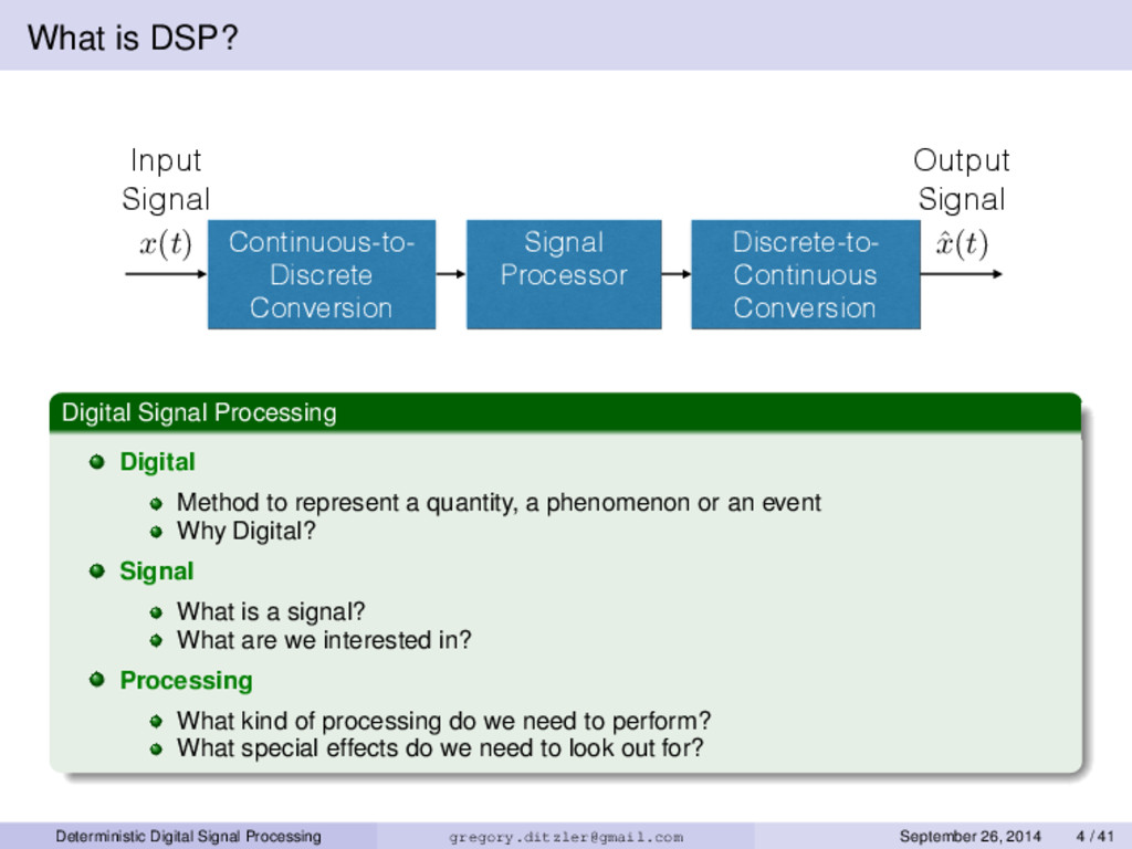
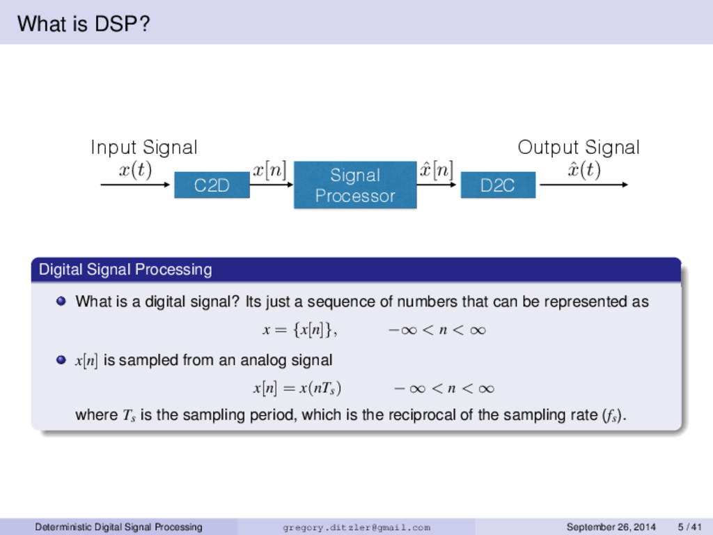
 Signal ˆ x(t) Continuous-to- Discrete Conversion Discrete-to- Continuous Conversion Signal
 Processor Digital Signal Processing Digital Method to represent a quantity, a phenomenon or an event Why Digital? Signal What is a signal? What are we interested in? Processing What kind of processing do we need to perform? What special effects do we need to look out for? Deterministic Digital Signal Processing gregory.ditzler@gmail.com September 26, 2014 4 / 41
5. What is DSP? Input Signal x(t) Output Signal ˆ x(t) C2D D2C Signal
 Processor x[n] ˆ x[n] Digital Signal Processing What is a digital signal? Its just a sequence of numbers that can be represented as x = {x[n]}, −∞ < n < ∞ x[n] is sampled from an analog signal x[n] = x(nTs) − ∞ < n < ∞ where Ts is the sampling period, which is the reciprocal of the sampling rate (fs). Deterministic Digital Signal Processing gregory.ditzler@gmail.com September 26, 2014 5 / 41
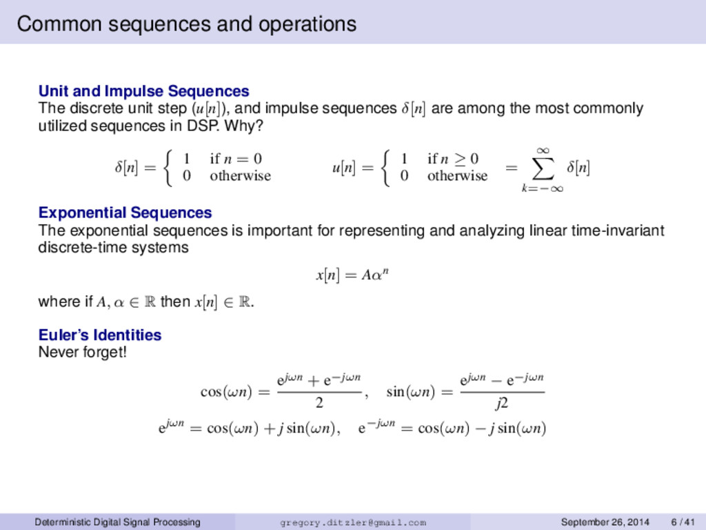
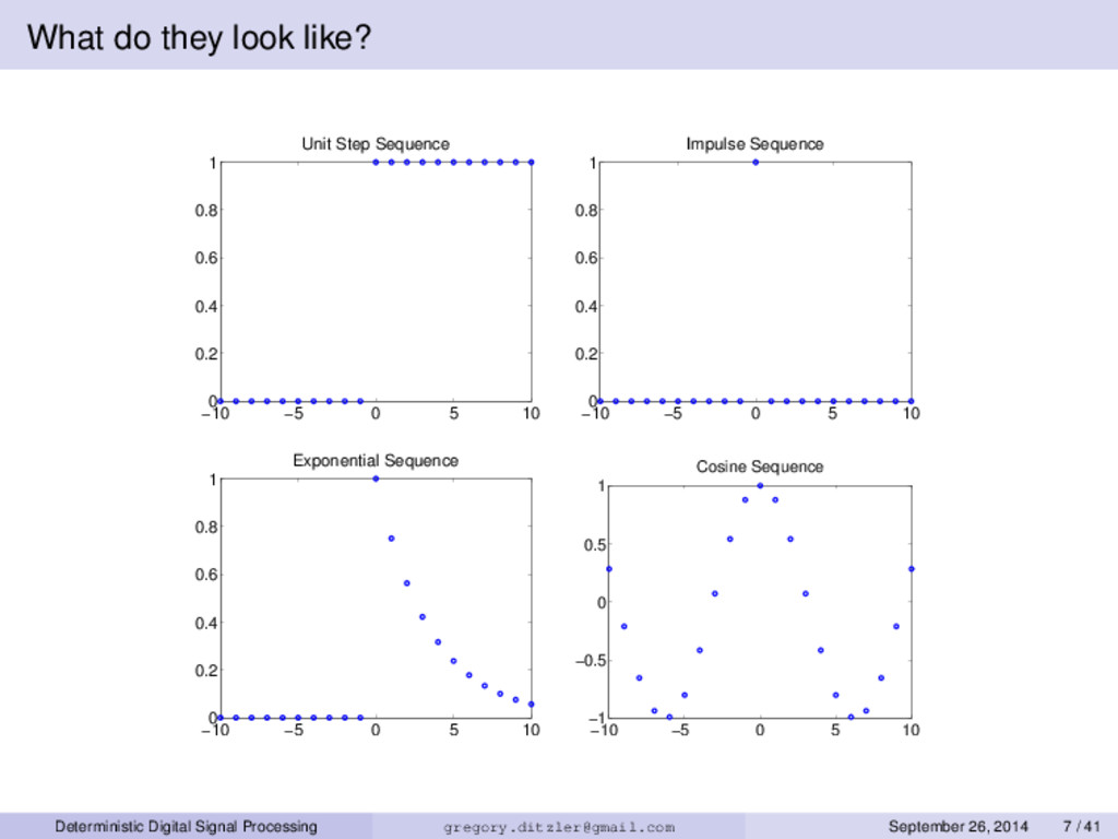
6. Common sequences and operations Unit and Impulse Sequences The discrete unit step (u[n]), and impulse sequences δ[n] are among the most commonly utilized sequences in DSP. Why? δ[n] = 1 if n = 0 0 otherwise u[n] = 1 if n ≥ 0 0 otherwise = ∞ k=−∞ δ[n] Exponential Sequences The exponential sequences is important for representing and analyzing linear time-invariant discrete-time systems x[n] = Aαn where if A, α ∈ R then x[n] ∈ R. Euler’s Identities Never forget! cos(ωn) = ejωn + e−jωn 2 , sin(ωn) = ejωn − e−jωn j2 ejωn = cos(ωn) + j sin(ωn), e−jωn = cos(ωn) − j sin(ωn) Deterministic Digital Signal Processing gregory.ditzler@gmail.com September 26, 2014 6 / 41
7. What do they look like? −10 −5 0 5 10 0 0.2 0.4 0.6 0.8 1 Unit Step Sequence −10 −5 0 5 10 0 0.2 0.4 0.6 0.8 1 Impulse Sequence −10 −5 0 5 10 0 0.2 0.4 0.6 0.8 1 Exponential Sequence −10 −5 0 5 10 −1 −0.5 0 0.5 1 Cosine Sequence Deterministic Digital Signal Processing gregory.ditzler@gmail.com September 26, 2014 7 / 41
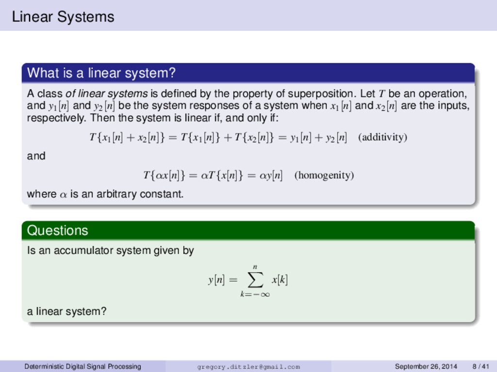
8. Linear Systems What is a linear system? A class of linear systems is defined by the property of superposition. Let T be an operation, and y1[n] and y2[n] be the system responses of a system when x1[n] and x2[n] are the inputs, respectively. Then the system is linear if, and only if: T{x1[n] + x2[n]} = T{x1[n]} + T{x2[n]} = y1[n] + y2[n] (additivity) and T{αx[n]} = αT{x[n]} = αy[n] (homogenity) where α is an arbitrary constant. Questions Is an accumulator system given by y[n] = n k=−∞ x[k] a linear system? Deterministic Digital Signal Processing gregory.ditzler@gmail.com September 26, 2014 8 / 41
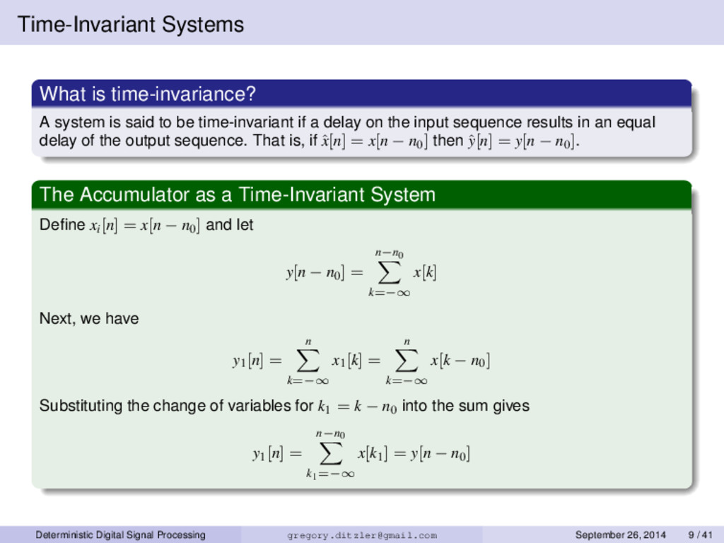
9. Time-Invariant Systems What is time-invariance? A system is said to be time-invariant if a delay on the input sequence results in an equal delay of the output sequence. That is, if ˆ x[n] = x[n − n0] then ˆ y[n] = y[n − n0]. The Accumulator as a Time-Invariant System Define xi[n] = x[n − n0] and let y[n − n0] = n−n0 k=−∞ x[k] Next, we have y1[n] = n k=−∞ x1[k] = n k=−∞ x[k − n0] Substituting the change of variables for k1 = k − n0 into the sum gives y1[n] = n−n0 k1=−∞ x[k1] = y[n − n0] Deterministic Digital Signal Processing gregory.ditzler@gmail.com September 26, 2014 9 / 41
10. Other Important Stuff Causality A system is casual if, for every choice of n0 , the output sequence value at the index n = n0 depends only of the input sequence values for n ≤ n0 . Is y[n] = x[n + 1] − x[n] causal? How about y[n] = log(x[|n| − n0])? Stability A system is bounded-input bounded-output (BIBO) stable if and only if every bounded input sequence results in a bounded output sequence. Everything else Seriously, read Chapter 2 of the text book! Deterministic Digital Signal Processing gregory.ditzler@gmail.com September 26, 2014 10 / 41
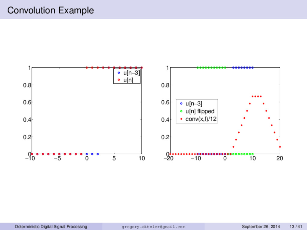
11. Linear Time-Invariant Systems What are they? As the name states, these systems are linear and time-invariant. They are one of the most important components to the field of digital signal processing. An LTI system can be completely characterized by its impulse response. That is, x[n] = δ[n]. Convolution The convolution of two sequences x and h is defined by: y[n] = ∞ k=−∞ x[k]h[n − k] = x[n] h[n] The importance of the equation shown above cannot be overstated enough Deterministic Digital Signal Processing gregory.ditzler@gmail.com September 26, 2014 11 / 41
12. Convolution Example −10 −5 0 5 10 0 0.2 0.4 0.6 0.8 1 u[n] an u[n] −20 −10 0 10 20 0 1 2 3 4 u[n] an u[n] flipped conv(x,f) Deterministic Digital Signal Processing gregory.ditzler@gmail.com September 26, 2014 12 / 41
13. Convolution Example −10 −5 0 5 10 0 0.2 0.4 0.6 0.8 1 u[n−3] u[n] −20 −10 0 10 20 0 0.2 0.4 0.6 0.8 1 u[n−3] u[n] flipped conv(x,f)/12 Deterministic Digital Signal Processing gregory.ditzler@gmail.com September 26, 2014 13 / 41
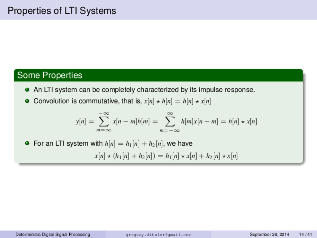
14. Properties of LTI Systems Some Properties An LTI system can be completely characterized by its impulse response. Convolution is commutative, that is, x[n] h[n] = h[n] x[n] y[n] = −∞ m=∞ x[n − m]h[m] = ∞ m=−∞ h[m]x[n − m] = h[n] x[n] For an LTI system with h[n] = h1[n] + h2[n], we have x[n] (h1[n] + h2[n]) = h1[n] x[n] + h2[n] x[n] Deterministic Digital Signal Processing gregory.ditzler@gmail.com September 26, 2014 14 / 41
15. Equivalence of LTI Systems x[n] y[n] h1 [n] h2 [n] h1 [n] ? h2 [n] = h2 [n] ? h1 [n] x[n] y[n] h1 [n] h2 [n] x[n] y[n] h1 [n] ? h2 [n] x[n] h1 [n] y[n] h2 [n] x[n] y[n] h1 [n] + h2 [n] Deterministic Digital Signal Processing gregory.ditzler@gmail.com September 26, 2014 15 / 41
16. LTI Examples: Moving Average y[n] = 1 L L−1 k=0 x[n − k] Linear?: Yes 1 L L−1 k=0 (ax1[n − k] + bx2[n − k]) = a 1 L L−1 k=0 x[n − k] + b 1 L L−1 k=0 x[n − k] Time-Invariant?: Yes 1 L L−1 k=0 x[n − k − n0] = 1 L L−1 k=0 x[(n − n0) − k] = y[n − n0] Casual?: Yes y[n] = 1 L (x[n] + x[n − 1] + . . . + x[n − L + 1]) BIBO?: Yes |y[n]| = 1 L L−1 k=0 x[n − k] ≤ 1 K L−1 k=0 |x[n − k]| ≤ Bx Deterministic Digital Signal Processing gregory.ditzler@gmail.com September 26, 2014 16 / 41
17. LTI Examples: Downsampler y[n] = x[Mn] Linear?: Yes ax1[Mn] + bx2[Mn] = ay1[n] + by2[n] Time-Invariant?: No y1[n] = x1[Mn] = x[Mn − n0] = y[n − n0] = x[M(n − n0)] Casual?: No y[−1] = x[−M], but y[1] = x[M] BIBO?: Yes |y[n]| = |x[Mn]| ≤ Bx Deterministic Digital Signal Processing gregory.ditzler@gmail.com September 26, 2014 17 / 41
18. LTI Systems Ideal Delay h[n] = δ[n − n0] Moving Average h[n] = 1 M1 + M2 + 1 M2 k=−M1 δ[n − k] = 1 M1+M2+1 −M1 ≤ n ≤ M2 0 otherwise Forward Difference h[n] = δ[n + 1] − δ[n] Backward Difference h[n] = δ[n] − δ[n − 1] Accumulator h[n] = M2 k=−M1 δ[k] = 1 n ≥ 0 0 n < 0 = u[n] Constant Coefficient Linear Difference N−1 k=0 aky[n − k] = M−1 m=0 bmx[n − m] Deterministic Digital Signal Processing gregory.ditzler@gmail.com September 26, 2014 18 / 41
19. Frequency Domain Representations of Discrete Signals Deterministic Digital Signal Processing gregory.ditzler@gmail.com September 26, 2014 19 / 41
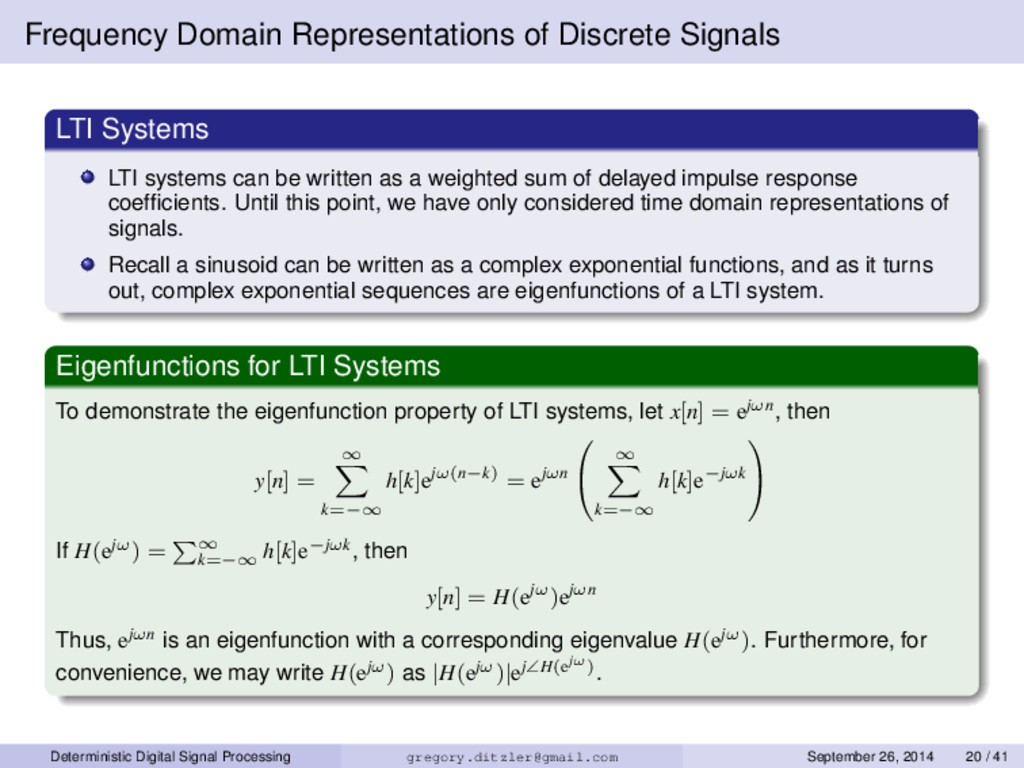
20. Frequency Domain Representations of Discrete Signals LTI Systems LTI systems can be written as a weighted sum of delayed impulse response coefficients. Until this point, we have only considered time domain representations of signals. Recall a sinusoid can be written as a complex exponential functions, and as it turns out, complex exponential sequences are eigenfunctions of a LTI system. Eigenfunctions for LTI Systems To demonstrate the eigenfunction property of LTI systems, let x[n] = ejωn, then y[n] = ∞ k=−∞ h[k]ejω(n−k) = ejωn   ∞ k=−∞ h[k]e−jωk   If H(ejω) = ∞ k=−∞ h[k]e−jωk, then y[n] = H(ejω)ejωn Thus, ejωn is an eigenfunction with a corresponding eigenvalue H(ejω). Furthermore, for convenience, we may write H(ejω) as |H(ejω)|ej∠H(ejω). Deterministic Digital Signal Processing gregory.ditzler@gmail.com September 26, 2014 20 / 41
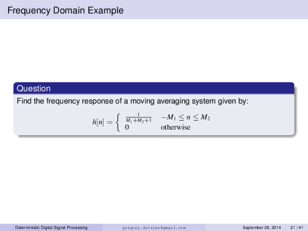
21. Frequency Domain Example Question Find the frequency response of a moving averaging system given by: h[n] = 1 M1+M2+1 −M1 ≤ n ≤ M2 0 otherwise Deterministic Digital Signal Processing gregory.ditzler@gmail.com September 26, 2014 21 / 41
22. Frequency Domain Example Therefore, the frequency response is given by H(ejω) = 1 M1 + M2 + 1 M2 n=−M1 e−jωn = 1 M1 + M2 + 1 ejωM1 − e−jω(M2+1) 1 − e−jω = 1 M1 + M2 + 1 ejω(M1+M2+1)/2 − e−jω(M1+M2+1)/2 1 − e−jω e−jω(M2−M1+1)/2 = 1 M1 + M2 + 1 ejω(M1+M2+1)/2 − e−jω(M1+M2+1)/2 ejω/2 − e−jω/2 e−jω(M2−M1)/2 = 1 M1 + M2 + 1 sin (ω(M1 + M2 + 1)/2) sin(ω/2) e−jω(M2−M1)/2 Deterministic Digital Signal Processing gregory.ditzler@gmail.com September 26, 2014 22 / 41
23. Frequency Domain Example −6 −4 −2 0 2 4 6 0 0.2 0.4 0.6 0.8 1 ω |H(ejω)| −6 −4 −2 0 2 4 6 −3 −2 −1 0 1 2 3 ω ∠ H(ejω) Deterministic Digital Signal Processing gregory.ditzler@gmail.com September 26, 2014 23 / 41
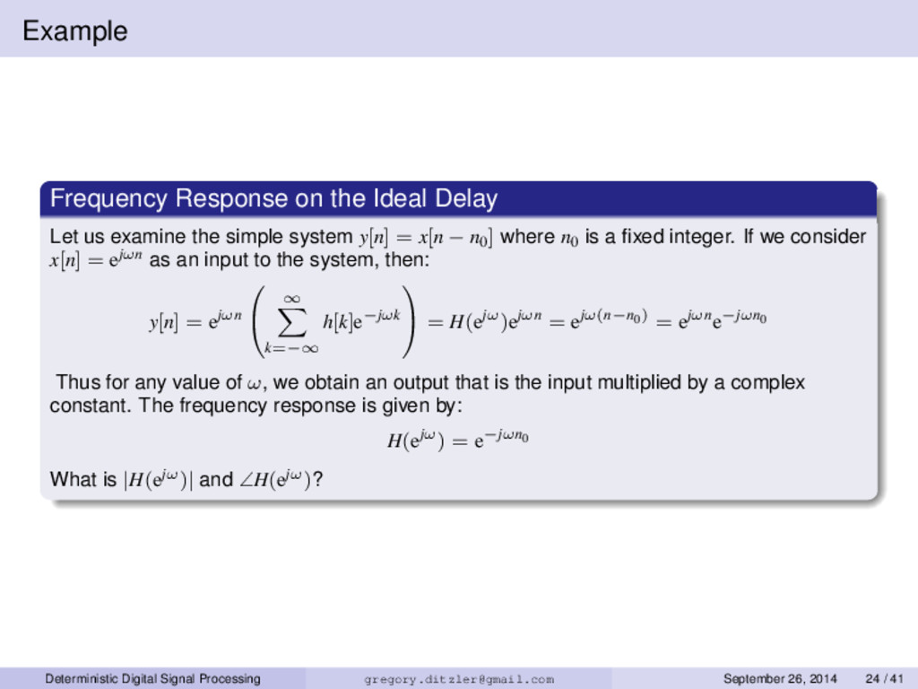
24. Example Frequency Response on the Ideal Delay Let us examine the simple system y[n] = x[n − n0] where n0 is a fixed integer. If we consider x[n] = ejωn as an input to the system, then: y[n] = ejωn   ∞ k=−∞ h[k]e−jωk   = H(ejω)ejωn = ejω(n−n0) = ejωne−jωn0 Thus for any value of ω, we obtain an output that is the input multiplied by a complex constant. The frequency response is given by: H(ejω) = e−jωn0 What is |H(ejω)| and ∠H(ejω)? Deterministic Digital Signal Processing gregory.ditzler@gmail.com September 26, 2014 24 / 41
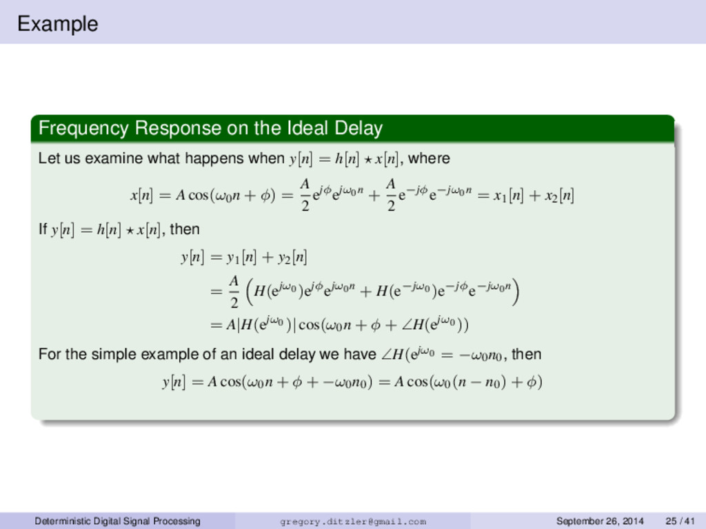
25. Example Frequency Response on the Ideal Delay Let us examine what happens when y[n] = h[n] x[n], where x[n] = A cos(ω0n + φ) = A 2 ejφejω0n + A 2 e−jφe−jω0n = x1[n] + x2[n] If y[n] = h[n] x[n], then y[n] = y1[n] + y2[n] = A 2 H(ejω0 )ejφejω0n + H(e−jω0 )e−jφe−jω0n = A|H(ejω0 )| cos(ω0n + φ + ∠H(ejω0 )) For the simple example of an ideal delay we have ∠H(ejω0 = −ω0n0 , then y[n] = A cos(ω0n + φ + −ω0n0) = A cos(ω0(n − n0) + φ) Deterministic Digital Signal Processing gregory.ditzler@gmail.com September 26, 2014 25 / 41
26. Historical Note: The 1889 World’s Fair in Paris, France Deterministic Digital Signal Processing gregory.ditzler@gmail.com September 26, 2014 26 / 41
27. And Who Made the List? Deterministic Digital Signal Processing gregory.ditzler@gmail.com September 26, 2014 27 / 41
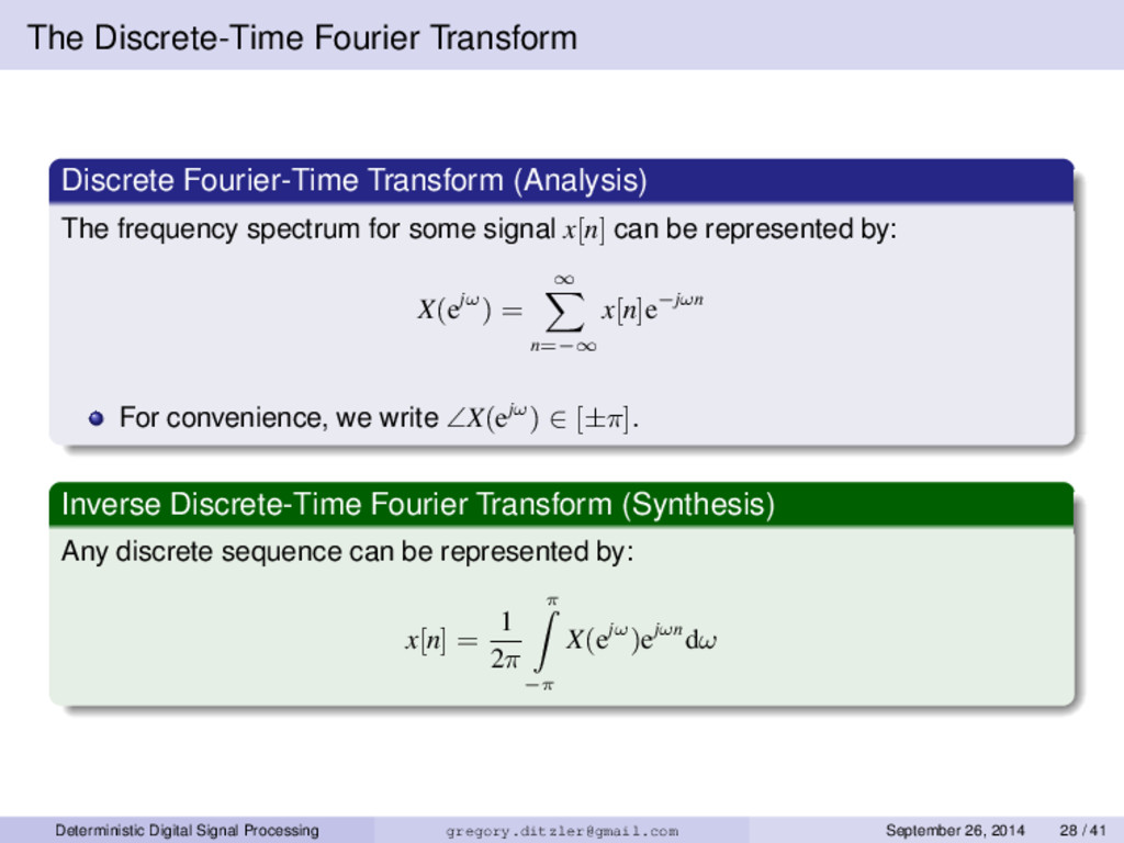
28. The Discrete-Time Fourier Transform Discrete Fourier-Time Transform (Analysis) The frequency spectrum for some signal x[n] can be represented by: X(ejω) = ∞ n=−∞ x[n]e−jωn For convenience, we write ∠X(ejω) ∈ [±π]. Inverse Discrete-Time Fourier Transform (Synthesis) Any discrete sequence can be represented by: x[n] = 1 2π π −π X(ejω)ejωndω Deterministic Digital Signal Processing gregory.ditzler@gmail.com September 26, 2014 28 / 41
29. Example Absolute Summability for a Suddenly-Applied Exponential Let x[n] = anu[n]. The Discrete-Time Fourier transform of this sequence is X(ejω) = ∞ n=−∞ x[n]e−jωn = ∞ n=0 ane−jωn = ∞ n=0 ae−jω n = 1 1 − ae−jω if |ae−jω| < 1 or a < 1. Clearly, the condition a < 1 is the condition for the absolute summability of x[n]; i.e., ∞ n=0 |a|n = 1 1 − |a| < ∞ again, only if a < 1. Deterministic Digital Signal Processing gregory.ditzler@gmail.com September 26, 2014 29 / 41
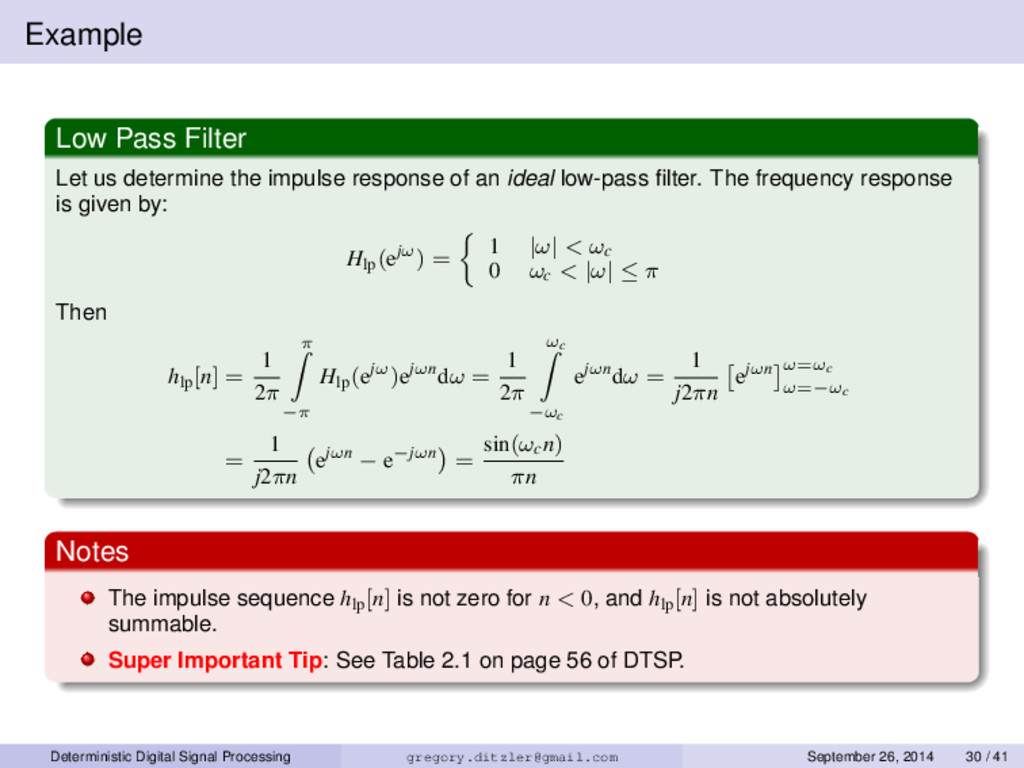
30. Example Low Pass Filter Let us determine the impulse response of an ideal low-pass filter. The frequency response is given by: Hlp(ejω) = 1 |ω| < ωc 0 ωc < |ω| ≤ π Then hlp[n] = 1 2π π −π Hlp(ejω)ejωndω = 1 2π ωc −ωc ejωndω = 1 j2πn ejωn ω=ωc ω=−ωc = 1 j2πn ejωn − e−jωn = sin(ωcn) πn Notes The impulse sequence hlp[n] is not zero for n < 0, and hlp[n] is not absolutely summable. Super Important Tip: See Table 2.1 on page 56 of DTSP. Deterministic Digital Signal Processing gregory.ditzler@gmail.com September 26, 2014 30 / 41
31. Example of Gibbs Phenomenon −4 −2 0 2 4 0 0.2 0.4 0.6 0.8 1 1.2 ω −4 −2 0 2 4 0 0.2 0.4 0.6 0.8 1 1.2 ω −4 −2 0 2 4 0 0.2 0.4 0.6 0.8 1 1.2 ω −4 −2 0 2 4 0 0.2 0.4 0.6 0.8 1 1.2 ω Deterministic Digital Signal Processing gregory.ditzler@gmail.com September 26, 2014 31 / 41
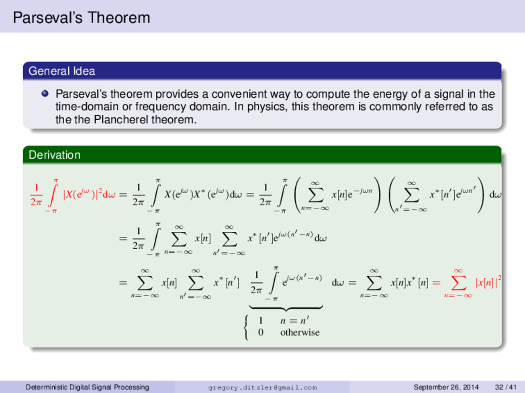
32. Parseval’s Theorem General Idea Parseval’s theorem provides a convenient way to compute the energy of a signal in the time-domain or frequency domain. In physics, this theorem is commonly referred to as the the Plancherel theorem. Derivation 1 2π π −π |X(ejω)|2dω = 1 2π π −π X(ejω)X∗(ejω)dω = 1 2π π −π   ∞ n=−∞ x[n]e−jωn     ∞ n =−∞ x∗[n ]ejωn   dω = 1 2π π −π ∞ n=−∞ x[n] ∞ n =−∞ x∗[n ]ejω(n −n)dω = ∞ n=−∞ x[n] ∞ n =−∞ x∗[n ] 1 2π π −π ejω(n −n)    1 n = n 0 otherwise dω = ∞ n=−∞ x[n]x∗[n] = ∞ n=−∞ |x[n]|2 Deterministic Digital Signal Processing gregory.ditzler@gmail.com September 26, 2014 32 / 41
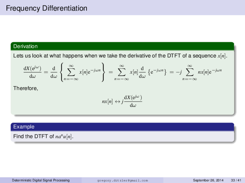
33. Frequency Differentiation Derivation Lets us look at what happens when we take the derivative of the DTFT of a sequence x[n]. dX(ejω) dω = d dω    ∞ n=−∞ x[n]e−jωn    = ∞ n=−∞ x[n] d dω e−jωn = −j ∞ n=−∞ nx[n]e−jωn Therefore, nx[n] ↔ j dX(ejω) dω Example Find the DTFT of nanu[n]. Deterministic Digital Signal Processing gregory.ditzler@gmail.com September 26, 2014 33 / 41
34. Properties of the Discrete-Time Fourier Transform A Few other use properties (x[n] ↔ X(ejω)) If y[n] = h[n] x[n] then Y(ejω) = H(ejω)X(ejω). This is the Convolution Theorem. Frequency Differentiation nx[n] ↔ j dX(ejω) dω Time Shifting x[n − n0] ↔ ejωn0 X(ejω) Frequency Shifting ejω0nx[n] ↔ X ej(ω−ω0) Convolutions x[n] y[n] ↔ X(ejω)Y(ejω) x[n]y[n] ↔ 1 2π π −π X(ejθ)Y(ej(ω−θ))dθ Deterministic Digital Signal Processing gregory.ditzler@gmail.com September 26, 2014 34 / 41
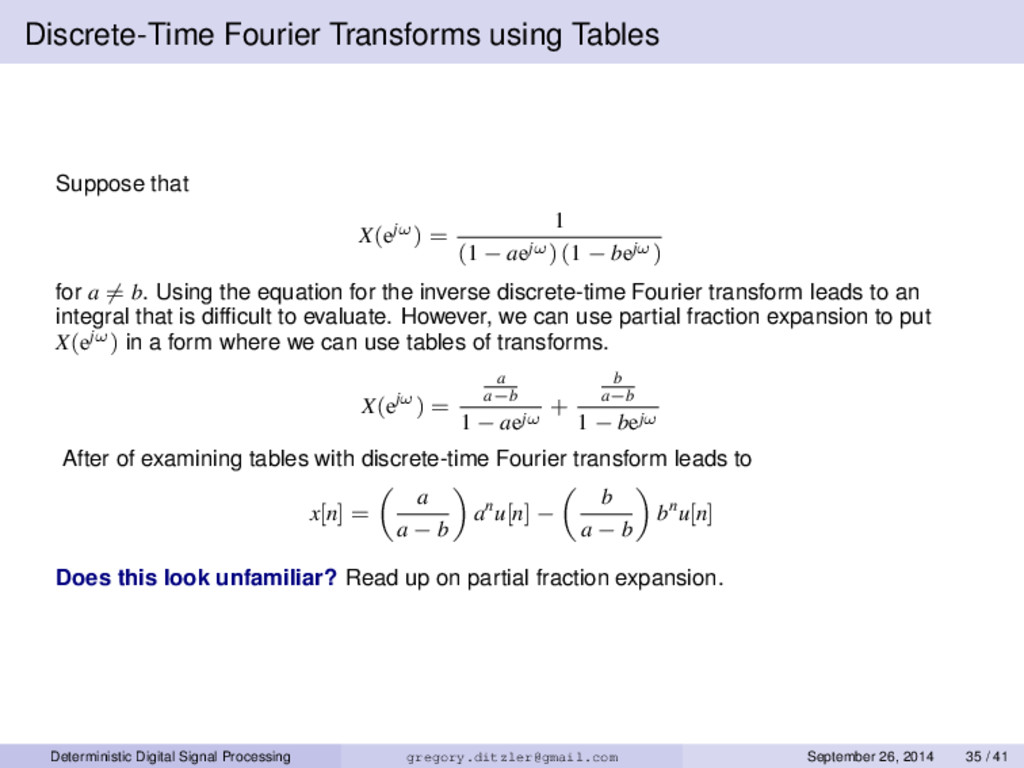
35. Discrete-Time Fourier Transforms using Tables Suppose that X(ejω) = 1 (1 − aejω) (1 − bejω) for a = b. Using the equation for the inverse discrete-time Fourier transform leads to an integral that is difficult to evaluate. However, we can use partial fraction expansion to put X(ejω) in a form where we can use tables of transforms. X(ejω) = a a−b 1 − aejω + b a−b 1 − bejω After of examining tables with discrete-time Fourier transform leads to x[n] = a a − b anu[n] − b a − b bnu[n] Does this look unfamiliar? Read up on partial fraction expansion. Deterministic Digital Signal Processing gregory.ditzler@gmail.com September 26, 2014 35 / 41
36. Example Determining the Impulse Response Given that y[n] = h[n] x[n], find h[n] when y[n] − 1 2 y[n − 1] = x[n] − 1 4 x[n − 1] −5 0 5 10 15 0 0.2 0.4 0.6 0.8 1 n h[n] Deterministic Digital Signal Processing gregory.ditzler@gmail.com September 26, 2014 36 / 41
37. Sampling 0 0.02 0.04 0.06 0.08 0.1 −5 0 5 (a) x(t) 0 0.02 0.04 0.06 0.08 0.1 −5 0 5 (b) sampled x(t) 0 20 40 60 80 100 0 20 40 60 80 100 120 140 (c) quantized signal 0 0.02 0.04 0.06 0.08 0.1 −5 0 5 (d) ˆ x(t) Deterministic Digital Signal Processing gregory.ditzler@gmail.com September 26, 2014 37 / 41
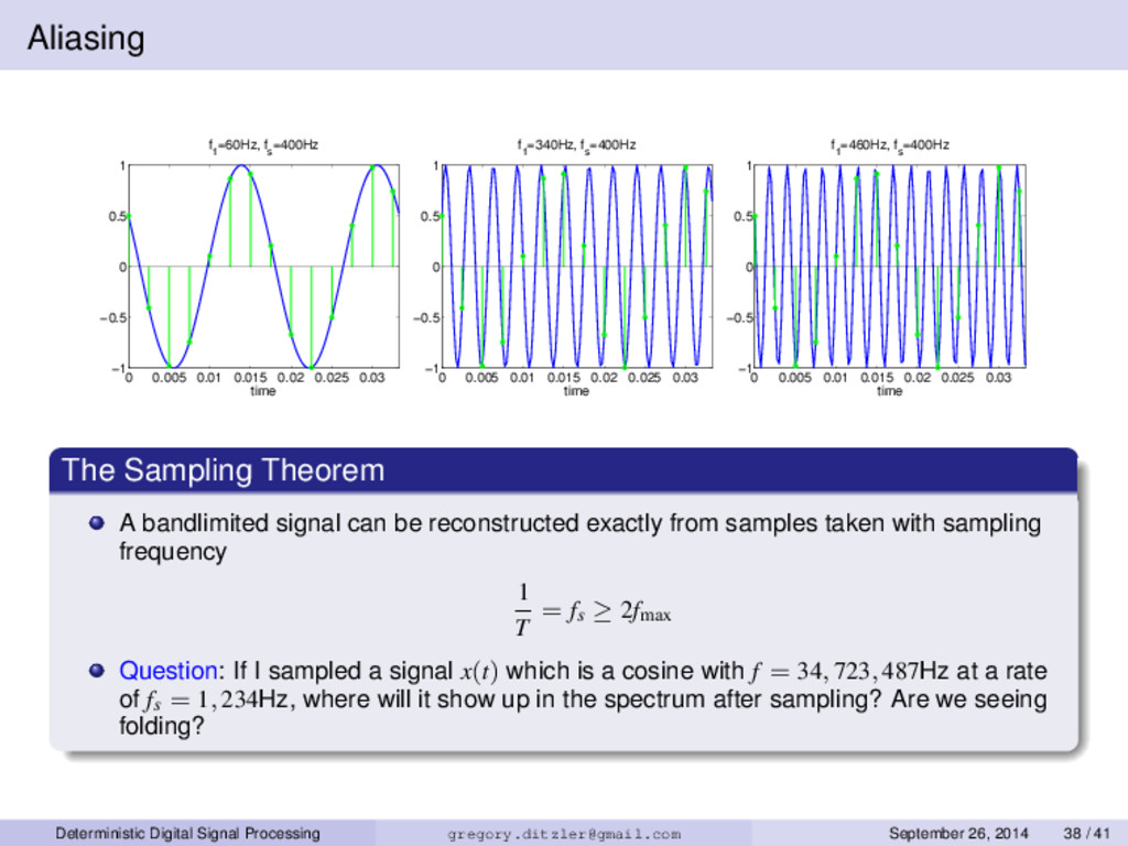
38. Aliasing 0 0.005 0.01 0.015 0.02 0.025 0.03 −1 −0.5 0 0.5 1 time f 1 =60Hz, f s =400Hz 0 0.005 0.01 0.015 0.02 0.025 0.03 −1 −0.5 0 0.5 1 f 1 =340Hz, f s =400Hz time 0 0.005 0.01 0.015 0.02 0.025 0.03 −1 −0.5 0 0.5 1 f 1 =460Hz, f s =400Hz time The Sampling Theorem A bandlimited signal can be reconstructed exactly from samples taken with sampling frequency 1 T = fs ≥ 2fmax Question: If I sampled a signal x(t) which is a cosine with f = 34, 723, 487Hz at a rate of fs = 1, 234Hz, where will it show up in the spectrum after sampling? Are we seeing folding? Deterministic Digital Signal Processing gregory.ditzler@gmail.com September 26, 2014 38 / 41
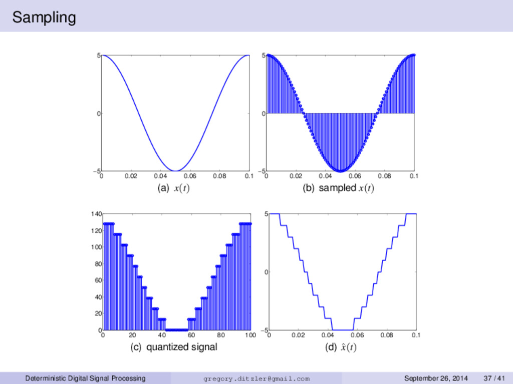
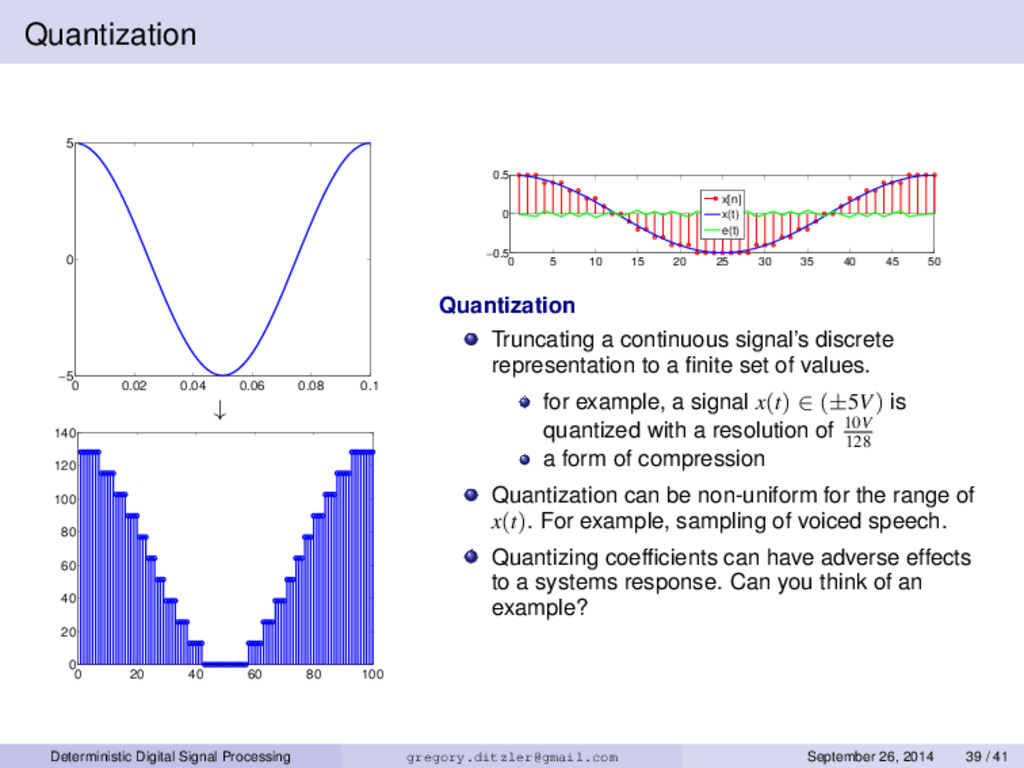
39. Quantization 0 0.02 0.04 0.06 0.08 0.1 −5 0 5 ↓ 0 20 40 60 80 100 0 20 40 60 80 100 120 140 0 5 10 15 20 25 30 35 40 45 50 −0.5 0 0.5 x[n] x(t) e(t) Quantization Truncating a continuous signal’s discrete representation to a finite set of values. for example, a signal x(t) ∈ (±5V) is quantized with a resolution of 10V 128 a form of compression Quantization can be non-uniform for the range of x(t). For example, sampling of voiced speech. Quantizing coefficients can have adverse effects to a systems response. Can you think of an example? Deterministic Digital Signal Processing gregory.ditzler@gmail.com September 26, 2014 39 / 41
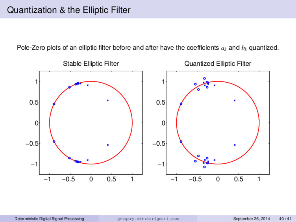
40. Quantization & the Elliptic Filter Pole-Zero plots of an elliptic filter before and after have the coefficients ak and bk quantized. −1 −0.5 0 0.5 1 −1 −0.5 0 0.5 1 Stable Elliptic Filter −1 −0.5 0 0.5 1 −1 −0.5 0 0.5 1 Quantized Elliptic Filter Deterministic Digital Signal Processing gregory.ditzler@gmail.com September 26, 2014 40 / 41
41. Quantization & the Elliptic Filter Frequency and phase response of an elliptic filter before and after have the coefficients ak and bk quantized. 0 0.5 1 −100 −80 −60 −40 −20 0 normalize frequency gain (dB) Original Quantized 0 0.5 1 −4 −2 0 2 4 normalize frequency phase (radians) Original Quantized Deterministic Digital Signal Processing gregory.ditzler@gmail.com September 26, 2014 41 / 41