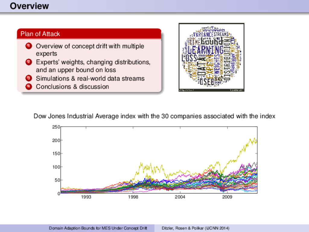
multiple experts 2 Experts’ weights, changing distributions, and an upper bound on loss 3 Simulations & real-world data streams 4 Conclusions & discussion Dow Jones Industrial Average index with the 30 companies associated with the index 1993 1998 2004 2009 0 50 100 150 200 250 Domain Adaption Bounds for MES Under Concept Drift Ditzler, Rosen & Polikar (IJCNN 2014)
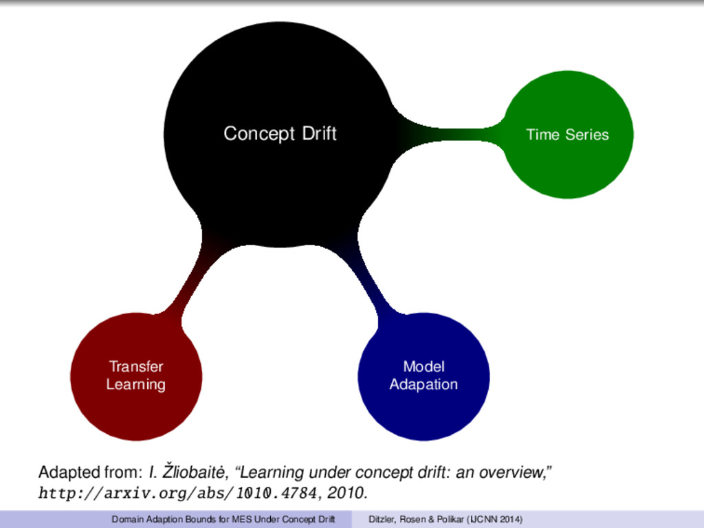
I. ˇ Zliobait˙ e, “Learning under concept drift: an overview,” http://arxiv.org/abs/1010.4784, 2010. Domain Adaption Bounds for MES Under Concept Drift Ditzler, Rosen & Polikar (IJCNN 2014)
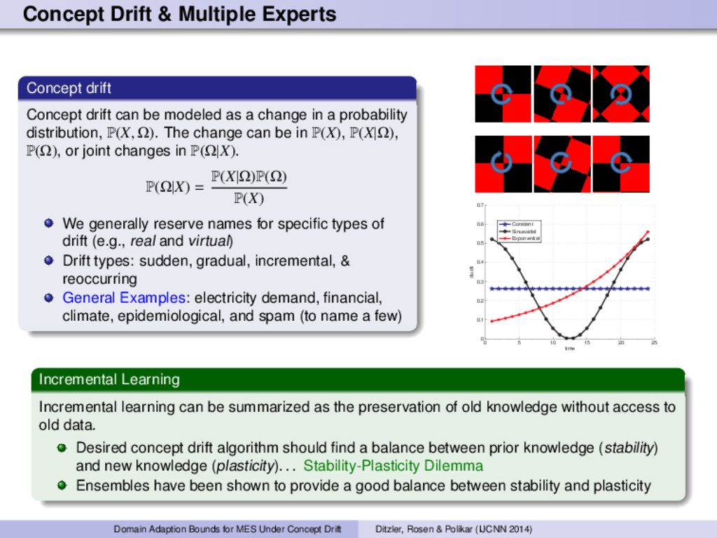
be modeled as a change in a probability distribution, P(X, Ω). The change can be in P(X), P(X|Ω), P(Ω), or joint changes in P(Ω|X). P(Ω|X) = P(X|Ω)P(Ω) P(X) We generally reserve names for specific types of drift (e.g., real and virtual) Drift types: sudden, gradual, incremental, & reoccurring General Examples: electricity demand, financial, climate, epidemiological, and spam (to name a few) 0 5 10 15 20 25 0 0.1 0.2 0.3 0.4 0.5 0.6 0.7 dα/dt time Constant Sinusoidal Exponential Incremental Learning Incremental learning can be summarized as the preservation of old knowledge without access to old data. Desired concept drift algorithm should find a balance between prior knowledge (stability) and new knowledge (plasticity). . . Stability-Plasticity Dilemma Ensembles have been shown to provide a good balance between stability and plasticity Domain Adaption Bounds for MES Under Concept Drift Ditzler, Rosen & Polikar (IJCNN 2014)
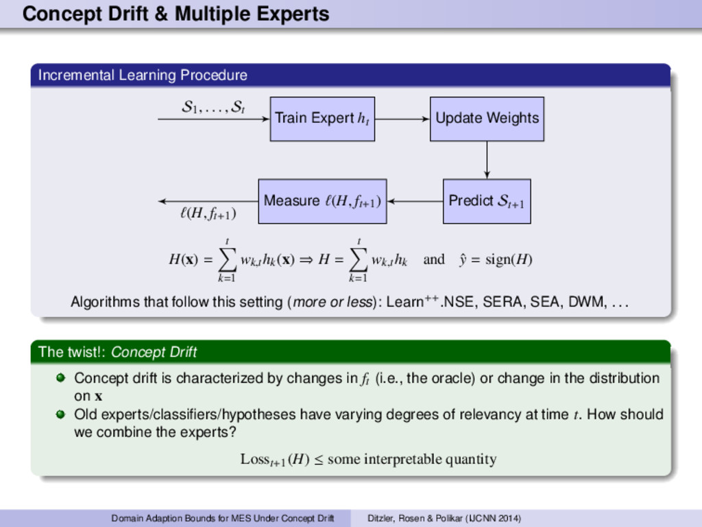
ht Update Weights Predict St+1 Measure (H, ft+1) S1 , . . . , St (H, ft+1) H(x) = t k=1 wk,thk(x) ⇒ H = t k=1 wk,thk and ˆ y = sign(H) Algorithms that follow this setting (more or less): Learn++.NSE, SERA, SEA, DWM, . . . The twist!: Concept Drift Concept drift is characterized by changes in ft (i.e., the oracle) or change in the distribution on x Old experts/classifiers/hypotheses have varying degrees of relevancy at time t. How should we combine the experts? Losst+1(H) ≤ some interpretable quantity Domain Adaption Bounds for MES Under Concept Drift Ditzler, Rosen & Polikar (IJCNN 2014)
for a classifier in an ensemble is typically of the form wk = log 1− k k where k is some expected measure of loss for the kth classifier. How do the expert weights affect the loss when being tested on an unknown distribution? Divergences and Bounds The H∆H distance measures the maximum difference in expected loss between h, h ∈ H, on two distributions (Kifer et al.) dH∆H (DT , Dk ) = 2 sup h,h ∈H |ET [ (h, h )] − Ek [ (h, h )]| Ben-David et al. bounded the loss of a single hypothesis being evaluated on an unknown distribution. ET (h, fT ) ≤ ES (h, f) + λ + 1 2 dH∆H (UT , US ) 0 5 10 x 105 0 0.5 1 1.5 2 2.5 3 N VC confidence ν=100 ν=200 ν=500 ν=5000 Domain Adaption Bounds for MES Under Concept Drift Ditzler, Rosen & Polikar (IJCNN 2014)
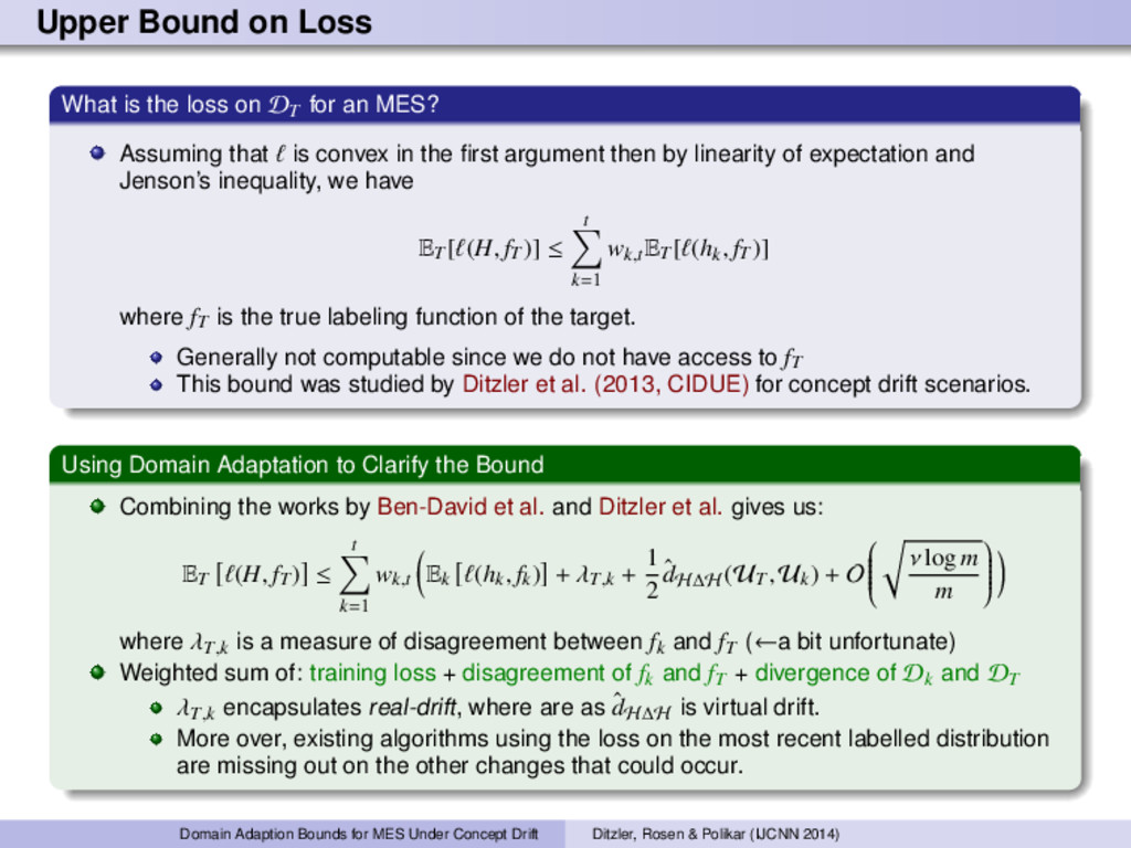
for an MES? Assuming that is convex in the first argument then by linearity of expectation and Jenson’s inequality, we have ET [ (H, fT )] ≤ t k=1 wk,tET [ (hk , fT )] where fT is the true labeling function of the target. Generally not computable since we do not have access to fT This bound was studied by Ditzler et al. (2013, CIDUE) for concept drift scenarios. Using Domain Adaptation to Clarify the Bound Combining the works by Ben-David et al. and Ditzler et al. gives us: ET (H, fT ) ≤ t k=1 wk,t Ek (hk , fk) + λT,k + 1 2 ˆ dH∆H (UT , Uk) + O ν log m m where λT,k is a measure of disagreement between fk and fT (←a bit unfortunate) Weighted sum of: training loss + disagreement of fk and fT + divergence of Dk and DT λT,k encapsulates real-drift, where are as ˆ dH∆H is virtual drift. More over, existing algorithms using the loss on the most recent labelled distribution are missing out on the other changes that could occur. Domain Adaption Bounds for MES Under Concept Drift Ditzler, Rosen & Polikar (IJCNN 2014)
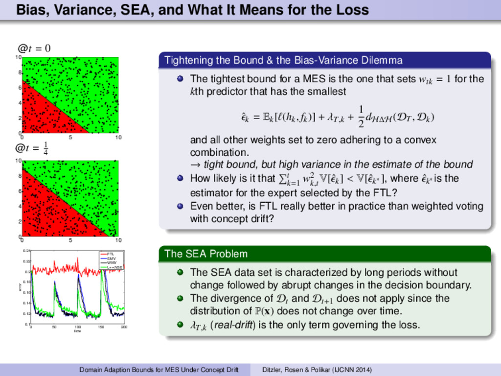
@t = 0 0 5 10 0 2 4 6 8 10 @t = 1 4 0 5 10 0 2 4 6 8 10 0 50 100 150 200 0.1 0.12 0.14 0.16 0.18 0.2 0.22 0.24 time error FTL SMV WMV L++.NSE Tightening the Bound & the Bias-Variance Dilemma The tightest bound for a MES is the one that sets wtk = 1 for the kth predictor that has the smallest ˆk = Ek[ (hk , fk)] + λT,k + 1 2 dH∆H (DT , Dk) and all other weights set to zero adhering to a convex combination. → tight bound, but high variance in the estimate of the bound How likely is it that t k=1 w2 k,tV[ˆk] < V[ˆk∗ ], where ˆk∗ is the estimator for the expert selected by the FTL? Even better, is FTL really better in practice than weighted voting with concept drift? The SEA Problem The SEA data set is characterized by long periods without change followed by abrupt changes in the decision boundary. The divergence of Dt and Dt+1 does not apply since the distribution of P(x) does not change over time. λT,k (real-drift) is the only term governing the loss. Domain Adaption Bounds for MES Under Concept Drift Ditzler, Rosen & Polikar (IJCNN 2014)
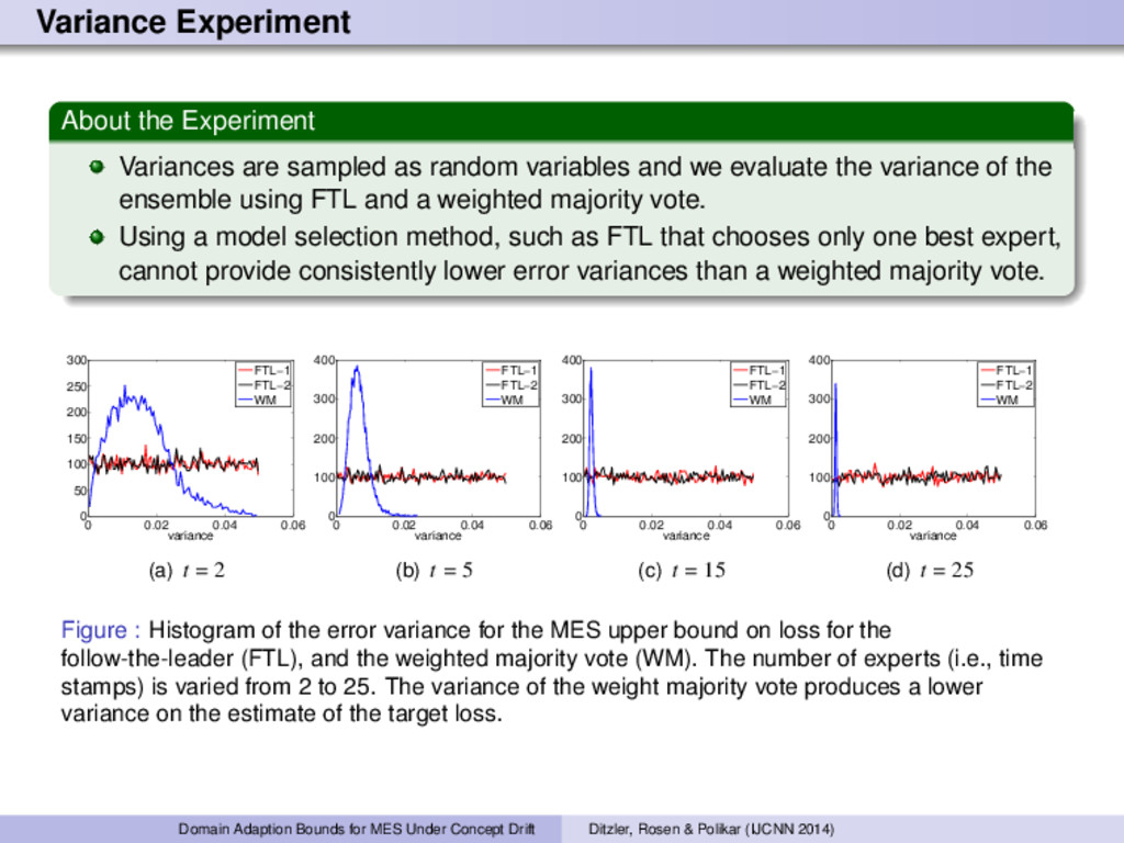
variables and we evaluate the variance of the ensemble using FTL and a weighted majority vote. Using a model selection method, such as FTL that chooses only one best expert, cannot provide consistently lower error variances than a weighted majority vote. 0 0.02 0.04 0.06 0 50 100 150 200 250 300 variance FTL−1 FTL−2 WM (a) t = 2 0 0.02 0.04 0.06 0 100 200 300 400 variance FTL−1 FTL−2 WM (b) t = 5 0 0.02 0.04 0.06 0 100 200 300 400 variance FTL−1 FTL−2 WM (c) t = 15 0 0.02 0.04 0.06 0 100 200 300 400 variance FTL−1 FTL−2 WM (d) t = 25 Figure : Histogram of the error variance for the MES upper bound on loss for the follow-the-leader (FTL), and the weighted majority vote (WM). The number of experts (i.e., time stamps) is varied from 2 to 25. The variance of the weight majority vote produces a lower variance on the estimate of the target loss. Domain Adaption Bounds for MES Under Concept Drift Ditzler, Rosen & Polikar (IJCNN 2014)
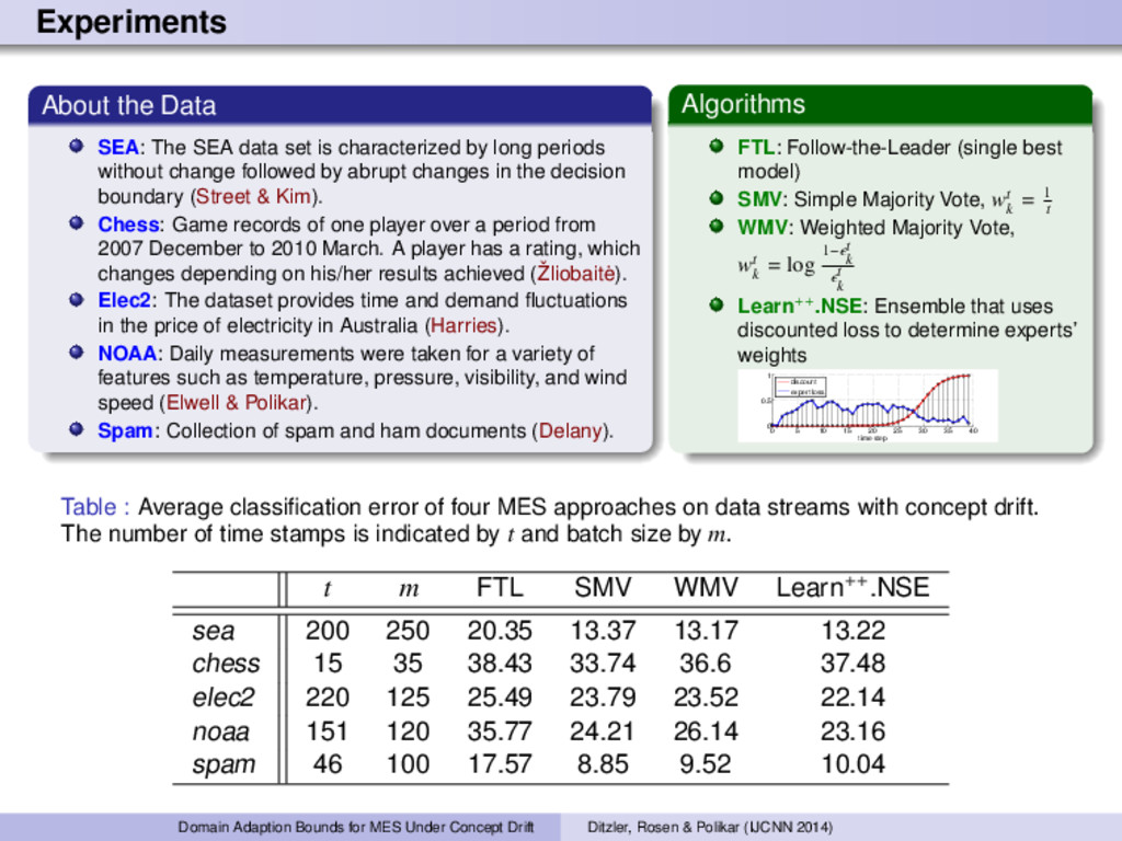
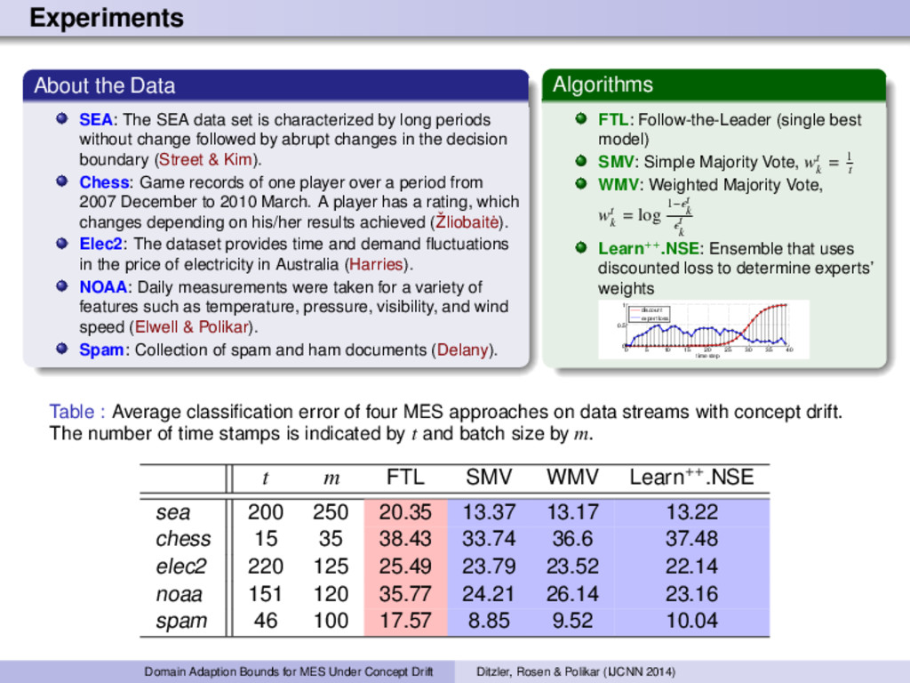
characterized by long periods without change followed by abrupt changes in the decision boundary (Street & Kim). Chess: Game records of one player over a period from 2007 December to 2010 March. A player has a rating, which changes depending on his/her results achieved (ˇ Zliobait˙ e). Elec2: The dataset provides time and demand fluctuations in the price of electricity in Australia (Harries). NOAA: Daily measurements were taken for a variety of features such as temperature, pressure, visibility, and wind speed (Elwell & Polikar). Spam: Collection of spam and ham documents (Delany). Algorithms FTL: Follow-the-Leader (single best model) SMV: Simple Majority Vote, wt k = 1 t WMV: Weighted Majority Vote, wt k = log 1− t k t k Learn++.NSE: Ensemble that uses discounted loss to determine experts’ weights 0 5 10 15 20 25 30 35 40 0 0.5 1 time step discount expert loss Table : Average classification error of four MES approaches on data streams with concept drift. The number of time stamps is indicated by t and batch size by m. t m FTL SMV WMV Learn++.NSE sea 200 250 20.35 13.37 13.17 13.22 chess 15 35 38.43 33.74 36.6 37.48 elec2 220 125 25.49 23.79 23.52 22.14 noaa 151 120 35.77 24.21 26.14 23.16 spam 46 100 17.57 8.85 9.52 10.04 Domain Adaption Bounds for MES Under Concept Drift Ditzler, Rosen & Polikar (IJCNN 2014)
characterized by long periods without change followed by abrupt changes in the decision boundary (Street & Kim). Chess: Game records of one player over a period from 2007 December to 2010 March. A player has a rating, which changes depending on his/her results achieved (ˇ Zliobait˙ e). Elec2: The dataset provides time and demand fluctuations in the price of electricity in Australia (Harries). NOAA: Daily measurements were taken for a variety of features such as temperature, pressure, visibility, and wind speed (Elwell & Polikar). Spam: Collection of spam and ham documents (Delany). Algorithms FTL: Follow-the-Leader (single best model) SMV: Simple Majority Vote, wt k = 1 t WMV: Weighted Majority Vote, wt k = log 1− t k t k Learn++.NSE: Ensemble that uses discounted loss to determine experts’ weights 0 5 10 15 20 25 30 35 40 0 0.5 1 time step discount expert loss Table : Average classification error of four MES approaches on data streams with concept drift. The number of time stamps is indicated by t and batch size by m. t m FTL SMV WMV Learn++.NSE sea 200 250 20.35 13.37 13.17 13.22 chess 15 35 38.43 33.74 36.6 37.48 elec2 220 125 25.49 23.79 23.52 22.14 noaa 151 120 35.77 24.21 26.14 23.16 spam 46 100 17.57 8.85 9.52 10.04 Domain Adaption Bounds for MES Under Concept Drift Ditzler, Rosen & Polikar (IJCNN 2014)
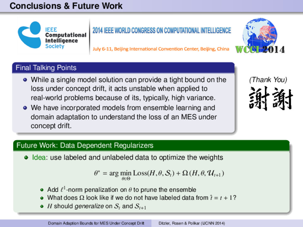
model solution can provide a tight bound on the loss under concept drift, it acts unstable when applied to real-world problems because of its, typically, high variance. We have incorporated models from ensemble learning and domain adaptation to understand the loss of an MES under concept drift. (Thank You) Future Work: Data Dependent Regularizers Idea: use labeled and unlabeled data to optimize the weights θ∗ = arg min θ∈Θ Loss(H, θ, St ) + Ω (H, θ, Ut+1 ) Add 1-norm penalization on θ to prune the ensemble What does Ω look like if we do not have labeled data from ˆ t = t + 1? H should generalize on St and St+1 Domain Adaption Bounds for MES Under Concept Drift Ditzler, Rosen & Polikar (IJCNN 2014)
Award #1310496. Any opinions, findings, and conclusions or recommendations expressed in this material are those of the author(s) and do not necessarily reflect the views of the National Science Foundation. Domain Adaption Bounds for MES Under Concept Drift Ditzler, Rosen & Polikar (IJCNN 2014)