Topics - Feature Selection

lecture notes on feature selection

Transcript

1. Introduction to Feature Selection Gregory Ditzler Drexel University Ecological and Evolutionary Signal Processing & Informatics Lab Department of Electrical & Computer Engineering Philadelphia, PA, USA gregory.ditzler@gmail.com http://github.com/gditzler/eces436-proteus April 29, 2014 Gregory Ditzler Introduction to Feature Selection
2. The material from these lecture notes was gathered from Gavin Brown’s feature selection lecture notes as well as other sources from the internet. Gregory Ditzler Introduction to Feature Selection
3. The plan for the next 45 minutes Overview Why subset selection? Examples? Algorithms for subset selection: wrapper, embedded and filter methods. How should I evaluate a subset selection algorithm? What does the current research look like? Time Permitting: Proteus examples (not feature selection related) Gregory Ditzler Introduction to Feature Selection
4. Motivation What are the input variables that ∗best∗ describe an outcome? Bacterial abundance profiles are collected from IBD and healthy patients. What are the bacteria that best differentiate between the two populations? Observations of a variable are not free. Which variables should I “pay” for, possibly in the future, to build a classifier? Gregory Ditzler Introduction to Feature Selection
5. More about this high dimensional world Examples There are an ever increasing number of applications that generate high dimensional data! Biometric authentication Pharmaceutical industries Systems biology Cancer diagnosis Metagenomics Gregory Ditzler Introduction to Feature Selection
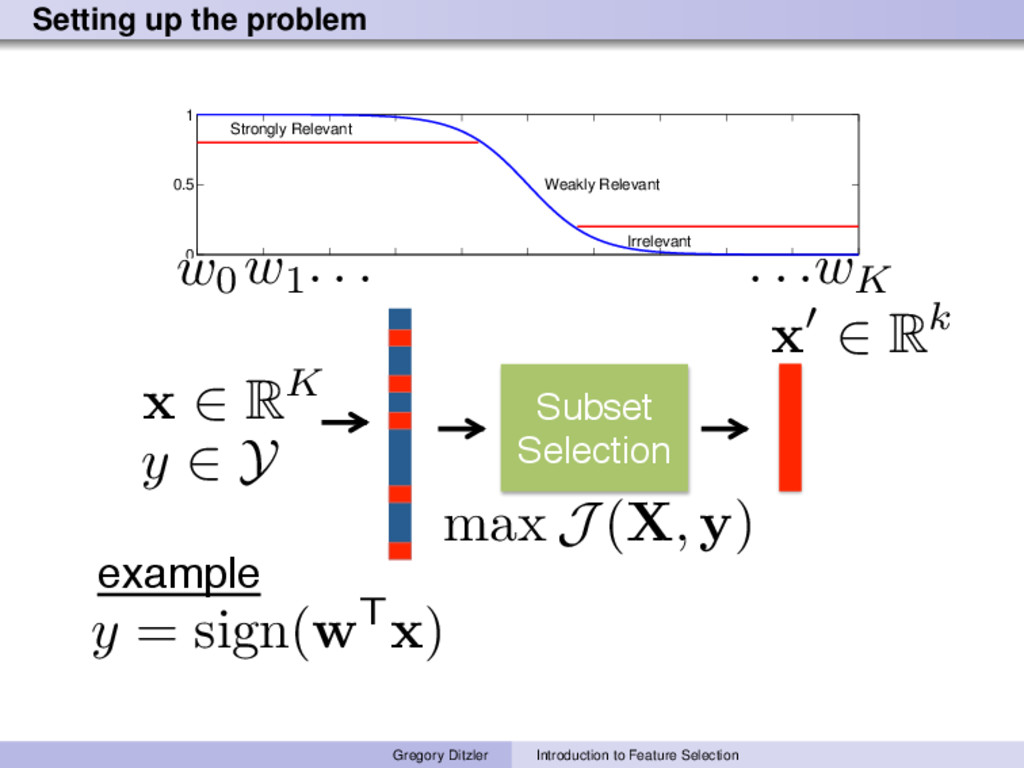
6. Supervised Learning Review from machine learning lecture In supervised learning, we learn a function to classify feature vectors from labeled training data. x: feature vector made up of variables X := {X1 , X2 , . . . , XK } y: label to a feature vector (e.g., y ∈ {+1, −1}) D: data set X = [x1 , x2 , . . . , xN ]T , y = [y1 , y2 , . . . , yN ]T Gregory Ditzler Introduction to Feature Selection
7. Setting up the problem Subset Selection! x 2 RK y 2 Y y = sign(wTx) −10 −8 −6 −4 −2 0 2 4 6 8 10 0 0.5 1 Strongly Relevant Irrelevant Weakly Relevant w0 w1 . . . wK . . . example! max J (X, y) x0 2 Rk Gregory Ditzler Introduction to Feature Selection
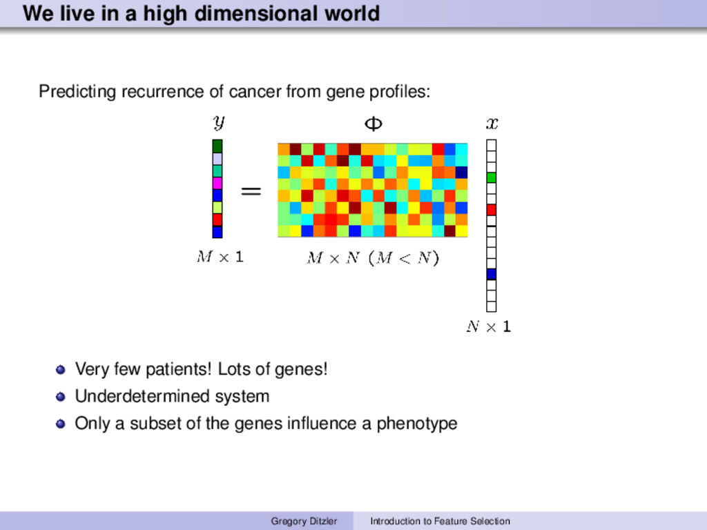
8. We live in a high dimensional world Predicting recurrence of cancer from gene profiles: Very few patients! Lots of genes! Underdetermined system Only a subset of the genes influence a phenotype Gregory Ditzler Introduction to Feature Selection
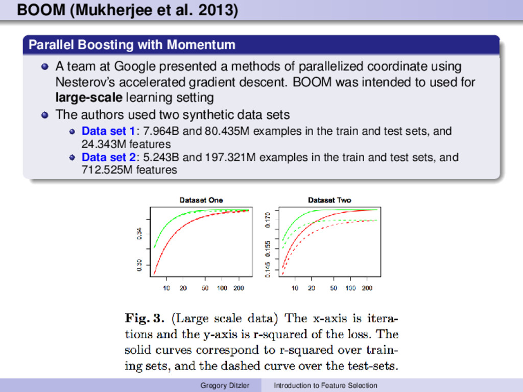
9. BOOM (Mukherjee et al. 2013) Parallel Boosting with Momentum A team at Google presented a methods of parallelized coordinate using Nesterov’s accelerated gradient descent. BOOM was intended to used for large-scale learning setting The authors used two synthetic data sets Data set 1: 7.964B and 80.435M examples in the train and test sets, and 24.343M features Data set 2: 5.243B and 197.321M examples in the train and test sets, and 712.525M features Gregory Ditzler Introduction to Feature Selection
10. Google maps (1024 × 1024 pixels) × (8 rotations) × (10 levels) = 83, 886, 080 features Gregory Ditzler Introduction to Feature Selection
11. Why subset selection? Why should we perform subset selection To improve accuracy of a classification or regression function. Subset selection does not always improve the accuracy of a classifier. Can you think of an example or reason why? Complexity of many machine learning algorithms scales with the number of features. Fewer features → lower complexity. Consider a classification algorithm who’s complexity is o( √ ND2). If you can work with D/50 features, then we have o( √ N(D/50)2) as the final complexity. Reduce cost of future measurements Improved data/model understanding Gregory Ditzler Introduction to Feature Selection
12. Feature Selection – Wrappers General Idea We have a classifier, and we would like to select a feature subset F ⊂ X that gives us a small loss. The subset selection wraps around the production of a classifier. Some wrappers, however, are classifier-dependent. Pro: Great performance! Con: computationally and memory expensive! Pseudo-Code Input: Feature select X, and identify a candidate set F ⊂ X. Evaluate the error of a classifier on F Adapt subset F Gregory Ditzler Introduction to Feature Selection
13. Question about the search space? If I have K features, how many different feature set combinations exist? Answer: 2K Gregory Ditzler Introduction to Feature Selection
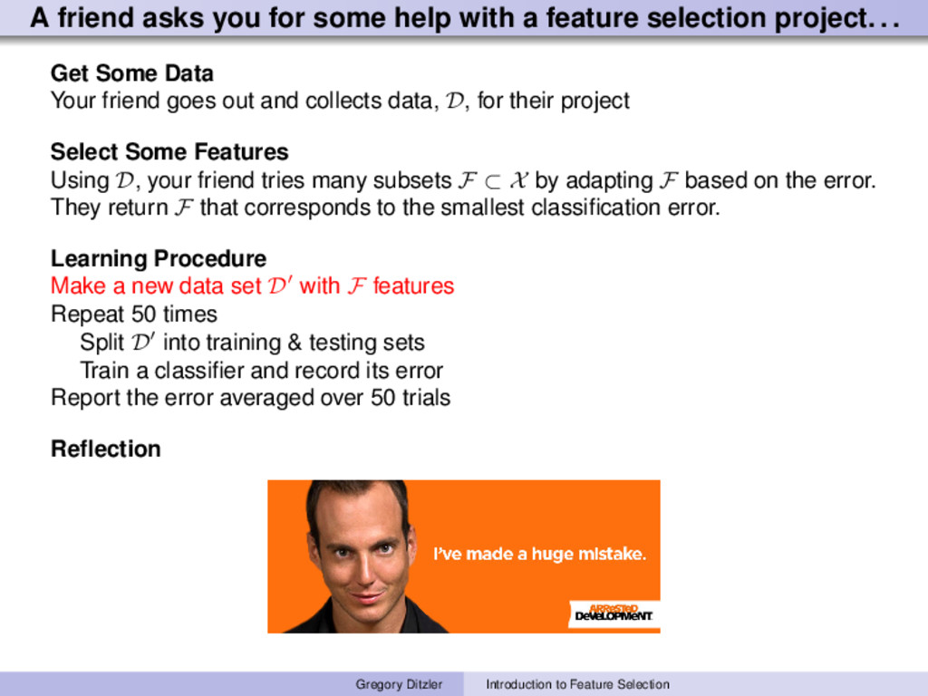
14. A friend asks you for some help with a feature selection project. . . Get Some Data Your friend goes out and collects data, D, for their project Select Some Features Using D, your friend tries many subsets F ⊂ X by adapting F based on the error. They return F that corresponds to the smallest classification error. Learning Procedure Make a new data set D with F features Repeat 50 times Split D into training & testing sets Train a classifier and record its error Report the error averaged over 50 trials Reflection Gregory Ditzler Introduction to Feature Selection
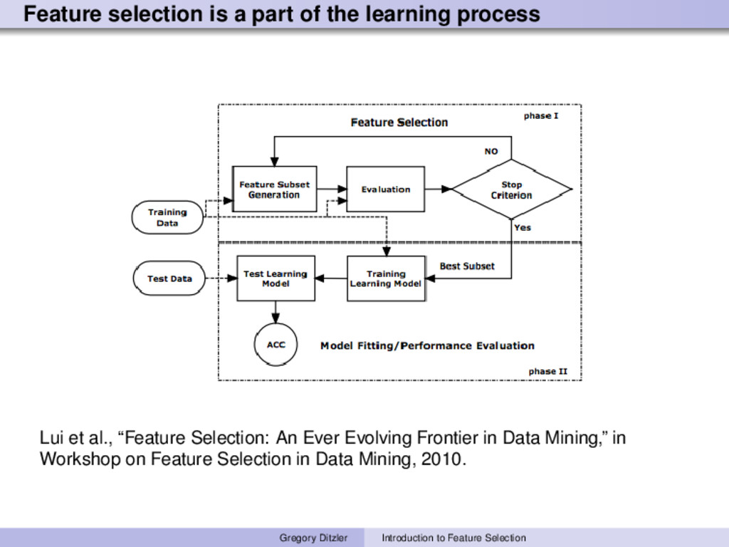
15. Feature selection is a part of the learning process Lui et al., “Feature Selection: An Ever Evolving Frontier in Data Mining,” in Workshop on Feature Selection in Data Mining, 2010. Gregory Ditzler Introduction to Feature Selection
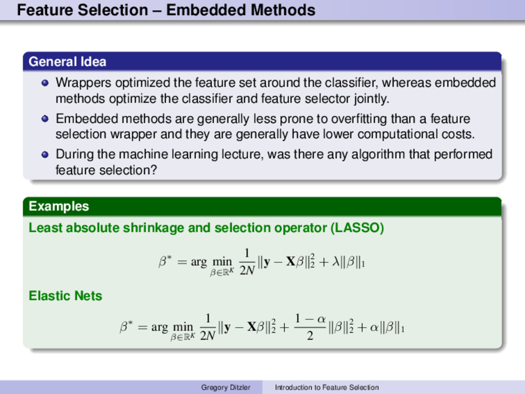
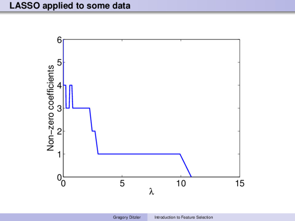
16. Feature Selection – Embedded Methods General Idea Wrappers optimized the feature set around the classifier, whereas embedded methods optimize the classifier and feature selector jointly. Embedded methods are generally less prone to overfitting than a feature selection wrapper and they are generally have lower computational costs. During the machine learning lecture, was there any algorithm that performed feature selection? Examples Least absolute shrinkage and selection operator (LASSO) β∗ = arg min β∈RK 1 2N y − Xβ 2 2 + λ β 1 Elastic Nets β∗ = arg min β∈RK 1 2N y − Xβ 2 2 + 1 − α 2 β 2 2 + α β 1 Gregory Ditzler Introduction to Feature Selection
17. LASSO applied to some data 10−2 100 0 50 100 150 200 250 λ MSE Gregory Ditzler Introduction to Feature Selection
18. LASSO applied to some data 0 5 10 15 0 1 2 3 4 5 6 λ Non−zero coefficients Gregory Ditzler Introduction to Feature Selection
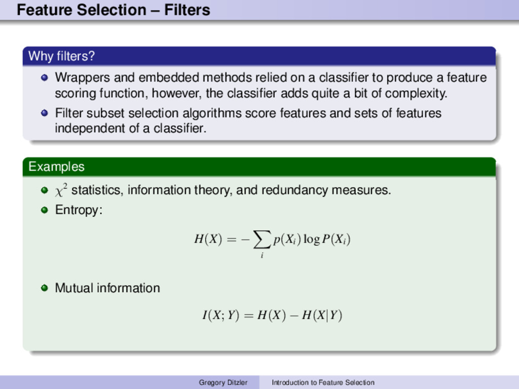
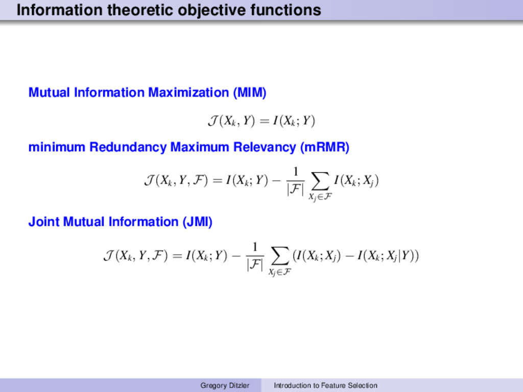
19. Feature Selection – Filters Why filters? Wrappers and embedded methods relied on a classifier to produce a feature scoring function, however, the classifier adds quite a bit of complexity. Filter subset selection algorithms score features and sets of features independent of a classifier. Examples χ2 statistics, information theory, and redundancy measures. Entropy: H(X) = − i p(Xi ) log P(Xi ) Mutual information I(X; Y) = H(X) − H(X|Y) Gregory Ditzler Introduction to Feature Selection
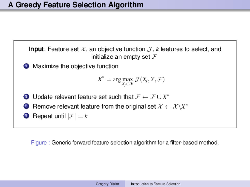
20. A Greedy Feature Selection Algorithm Input: Feature set X, an objective function J , k features to select, and initialize an empty set F 1 Maximize the objective function X∗ = arg max Xj∈X J (Xj , Y, F) 2 Update relevant feature set such that F ← F ∪ X∗ 3 Remove relevant feature from the original set X ← X\X∗ 4 Repeat until |F| = k Figure : Generic forward feature selection algorithm for a filter-based method. Gregory Ditzler Introduction to Feature Selection
21. Information theoretic objective functions Mutual Information Maximization (MIM) J (Xk , Y) = I(Xk ; Y) minimum Redundancy Maximum Relevancy (mRMR) J (Xk , Y, F) = I(Xk ; Y) − 1 |F| Xj∈F I(Xk ; Xj ) Joint Mutual Information (JMI) J (Xk , Y, F) = I(Xk ; Y) − 1 |F| Xj∈F (I(Xk ; Xj ) − I(Xk ; Xj |Y)) Gregory Ditzler Introduction to Feature Selection
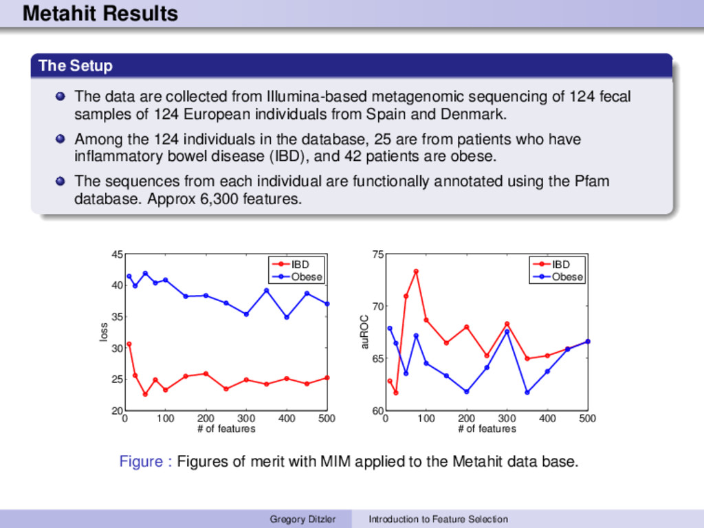
22. Metahit Results The Setup The data are collected from Illumina-based metagenomic sequencing of 124 fecal samples of 124 European individuals from Spain and Denmark. Among the 124 individuals in the database, 25 are from patients who have inflammatory bowel disease (IBD), and 42 patients are obese. The sequences from each individual are functionally annotated using the Pfam database. Approx 6,300 features. 0 100 200 300 400 500 20 25 30 35 40 45 # of features loss IBD Obese 0 100 200 300 400 500 60 65 70 75 # of features auROC IBD Obese Figure : Figures of merit with MIM applied to the Metahit data base. Gregory Ditzler Introduction to Feature Selection
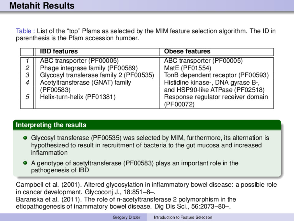
23. Metahit Results Table : List of the “top” Pfams as selected by the MIM feature selection algorithm. The ID in parenthesis is the Pfam accession humber. IBD features Obese features 1 ABC transporter (PF00005) ABC transporter (PF00005) 2 Phage integrase family (PF00589) MatE (PF01554) 3 Glycosyl transferase family 2 (PF00535) TonB dependent receptor (PF00593) 4 Acetyltransferase (GNAT) family Histidine kinase-, DNA gyrase B-, (PF00583) and HSP90-like ATPase (PF02518) 5 Helix-turn-helix (PF01381) Response regulator receiver domain (PF00072) Interpreting the results Glycosyl transferase (PF00535) was selected by MIM, furthermore, its alternation is hypothesized to result in recruitment of bacteria to the gut mucosa and increased inflammation A genotype of acetyltransferase (PF00583) plays an important role in the pathogenesis of IBD Campbell et al. (2001). Altered glycosylation in inflammatory bowel disease: a possible role in cancer development. Glycoconj J., 18:851–8–. Baranska et al. (2011). The role of n-acetyltransferase 2 polymorphism in the etiopathogenesis of inammatory bowel disease. Dig Dis Sci., 56:2073–80–. Gregory Ditzler Introduction to Feature Selection
24. The NPFS Algorithm ⇤(z) = P(Zn = z|H1 ) P(Zn = z|H0 ) = n z pz 1 (1 p1 )n z n z pz 0 (1 p0 )n z > ⇣crit Hypothesis Test Based on the Likelihood Ratio! H0 : p = p0 H1 : p > p0 Hypothesis Test! f1 f2 fK . . . . . . f3 Bootstrap! 1 2 3 4 n . . . Features! Chance ! p0 = k K X X1i = k X X2i = k X X3i = k X X4i = k X Xni = k {z}1 = X Xl1 {z}K = X XlK Gregory Ditzler Introduction to Feature Selection
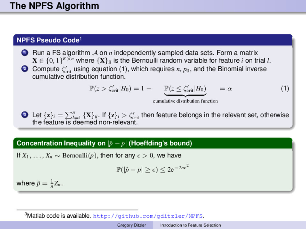
25. The NPFS Algorithm NPFS Pseudo Code1 1 Run a FS algorithm A on n independently sampled data sets. Form a matrix X ∈ {0, 1}K×n where {X}il is the Bernoulli random variable for feature i on trial l. 2 Compute ζ crit using equation (1), which requires n, p0 , and the Binomial inverse cumulative distribution function. P(z > ζcrit |H0) = 1 − P(z ≤ ζcrit |H0) cumulative distribution function = α (1) 3 Let {z}i = n l=1 {X}il . If {z}i > ζ crit then feature belongs in the relevant set, otherwise the feature is deemed non-relevant. Concentration Inequality on |ˆ p − p| (Hoeffding’s bound) If X1 , . . . , Xn ∼ Bernoulli(p), then for any > 0, we have P(|ˆ p − p| ≥ ) ≤ 2e−2n 2 where ˆ p = 1 n Zn. 3Matlab code is available. http://github.com/gditzler/NPFS. Gregory Ditzler Introduction to Feature Selection
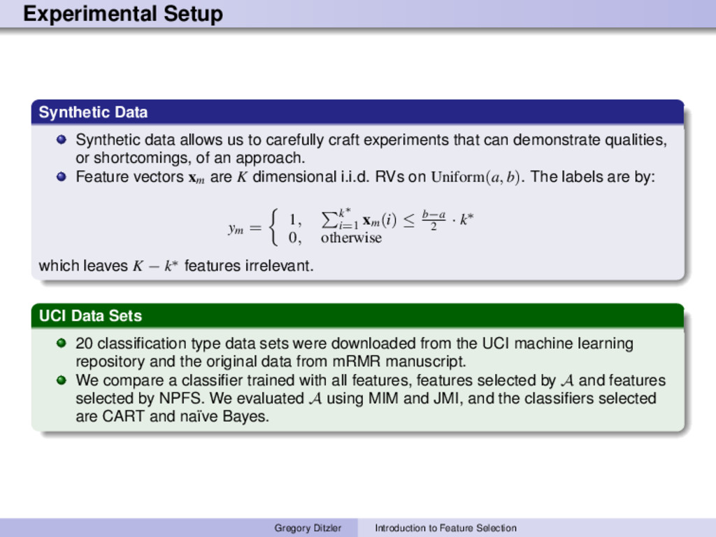
26. Experimental Setup Synthetic Data Synthetic data allows us to carefully craft experiments that can demonstrate qualities, or shortcomings, of an approach. Feature vectors xm are K dimensional i.i.d. RVs on Uniform(a, b). The labels are by: ym = 1, k∗ i=1 xm(i) ≤ b−a 2 · k∗ 0, otherwise which leaves K − k∗ features irrelevant. UCI Data Sets 20 classification type data sets were downloaded from the UCI machine learning repository and the original data from mRMR manuscript. We compare a classifier trained with all features, features selected by A and features selected by NPFS. We evaluated A using MIM and JMI, and the classifiers selected are CART and na¨ ıve Bayes. Gregory Ditzler Introduction to Feature Selection
27. Results on Synthetic Data 20 40 60 80 100 5 10 15 20 25 bootstrap feature (a) k = 10 20 40 60 80 100 5 10 15 20 25 bootstrap feature (b) k = 15 20 40 60 80 100 5 10 15 20 25 bootstrap feature (c) k = 20 20 40 60 80 100 5 10 15 20 25 bootstrap feature (d) k = 24 Figure : Visualization of X, where black segments indicate Xl = 0, white segments Xl = 1, and the orange rows are the features detected as relevant by NPFS. Note k∗ = 5. 0 100 200 300 400 500 0 5 10 15 20 25 number of bootstraps # features (max 50) k=3 k=5 k=10 k=15 k=25 (a) K = 50, k∗ = 15 0 100 200 300 400 500 0 5 10 15 20 25 number of bootstraps # features (max 100) k=3 k=5 k=10 k=15 k=25 (b) K = 100, k∗ = 15 0 100 200 300 400 500 0 10 20 30 40 number of bootstraps # features (max 250) k=3 k=5 k=10 k=15 k=25 (c) K = 250, k∗ = 15 Figure : Number of features selected by NPFS for varying levels of k. Gregory Ditzler Introduction to Feature Selection
28. Results on UCI Data data set |D| K nb nb-jmi nb-npfs cart cart-jmi cart-npfs breast 569 30 0.069 (3) 0.055 (1.5) 0.055 (1.5) 0.062 (3) 0.056 (2) 0.041 (1) congress 435 16 0.097 (3) 0.088 (1) 0.088 (2) 0.051 (3) 0.051 (1.5) 0.051 (1.5) heart 270 13 0.156 (1) 0.163 (2) 0.174 (3) 0.244 (3) 0.226 (2) 0.207 (1) ionosphere 351 34 0.117 (3) 0.091 (2) 0.091 (1) 0.077 (3) 0.068 (1) 0.074 (2) krvskp 3196 36 0.122 (3) 0.108 (1) 0.116 (2) 0.006 (1) 0.056 (3) 0.044 (2) landsat 6435 36 0.204 (1) 0.231 (2.5) 0.231 (2.5) 0.161 (1) 0.173 (2) 0.174 (3) lungcancer 32 56 0.617 (3) 0.525 (1) 0.617 (2) 0.542 (2) 0.558 (3) 0.533 (1) parkinsons 195 22 0.251 (3) 0.170 (1.5) 0.170 (1.5) 0.133 (1.5) 0.138 (3) 0.133 (1.5) pengcolon 62 2000 0.274 (3) 0.179 (2) 0.164 (1) 0.21 (1) 0.226 (2.5) 0.226 (2.5) pengleuk 72 7070 0.421 (3) 0.029 (1) 0.043 (2) 0.041 (2) 0.027 (1) 0.055 (3) penglung 73 325 0.107 (1) 0.368 (3) 0.229 (2) 0.337 (1) 0.530 (3) 0.504 (2) penglymp 96 4026 0.087 (1) 0.317 (3) 0.140 (2) 0.357 (3) 0.312 (2) 0.311 (1) pengnci9 60 9712 0.900 (3) 0.600 (2) 0.400 (1) 0.667 (2) 0.617 (1) 0.783 (3) semeion 1593 256 0.152 (1) 0.456 (3) 0.387 (2) 0.25 (1) 0.443 (3) 0.355 (2) sonar 208 60 0.294 (3) 0.279 (2) 0.241 (1) 0.259 (2) 0.263 (3) 0.201 (1) soybean 47 35 0.000 (2) 0.000 (2) 0.000 (2) 0.020 (2) 0.020 (2) 0.020 (2) spect 267 22 0.210 (2) 0.206 (1) 0.232 (3) 0.187 (1) 0.210 (2) 0.229 (3) splice 3175 60 0.044 (1) 0.054 (2) 0.055 (3) 0.085 (3) 0.070 (2) 0.066 (1) waveform 5000 40 0.207 (3) 0.204 (2) 0.202 (1) 0.259 (3) 0.238 (2) 0.228 (1) wine 178 13 0.039 (2.5) 0.039 (2.5) 0.034 (1) 0.079 (3) 0.068 (1.5) 0.068 (1.5) average 2.275 1.900 1.825 2.075 2.1250 1.800 Highlights CART+NPFS provides statistically significant improvement. NPFS (even after a large number of bootstraps) does not detect all features as important Gregory Ditzler Introduction to Feature Selection