Wouter Verkerke, Systematic uncertainties! and profiling

IN2P3 School of Statistics 2014
https://indico.in2p3.fr/event/9742/

Transcript

1. Wouter Verkerke, Nikhef Systematic uncertainties! and profiling Wouter Verkerke (Nikhef/Atlas)
2. Wouter Verkerke, NIKHEF The scope! of this course 0
3. Profiling & Systematics as part of statistical analysis •  A HEP analysis requires close integration of ‘physics concepts’ and ‘statistical concepts’ 1.  Design event selection “physics” •  Use simulated samples of signal, background to aid selection process ! (cuts, BDT, NN etc) 2.  Analyze (‘fit’) data in selection “statistics” •  Measurement with statistical error, limit based on statistical uncertainty 3.  Make inventory of systematic uncertainties “physics” •  Generally, any effect that isn’t measured constrained from your own measurement 4.  Finalize result ‘including systematics’ “statistics” •  Variety of (empirical/fundamental) approaches to do this 5.  Interpretation “physics” •  Better measurement, discovery etc, find mistake/sub-optimality in procedure •  Focus of this course: steps 3 and 4. –  Practical problem: ‘physics notion’ of systematic uncertainties does not map 1-1 to a statistical procedure. Many procedures exist, some ad-hoc, some rigorous (from the statistical p.o.v.) Wouter Verkerke, NIKHEF
4. Profiling & Systematics as part of statistical data analysis Wouter Verkerke, NIKHEF Systematic uncertainties Nuisance parameters The physicists world The statisticians world Profiling
5. Outline of this course •  Outline of this course 1.  What are systematic uncertainties? 2.  Incorporating systematic uncertainties in probability models 3.  Modeling shape systematics: template morphing 4.  Tools for modelling building RooFit/RooStats and HistFactory 5.  Diagnostics: Overconstraining & choices in model parametrization Wouter Verkerke, NIKHEF
6. Wouter Verkerke, NIKHEF What are ! systematic ! uncertainties? 1
7. What are systematic uncertainties? •  Concept & definitions of ‘systematic uncertainties’ originates from physics, not from fundamental statistical methodology. –  E.g. Glen Cowans (excellent) 198pp book “statistical data analysis” ! does not discuss systematic uncertainties at all! •  A common definition is –  “Systematic uncertainties are all uncertainties that are ! not directly due to the statistics of the data”! •  But the notion of ‘the data’ is a key source of ambiguity: –  does it include control measurements? –  does it include measurements that were used to perform basic ! (energy scale) calibrations? Wouter Verkerke, NIKHEF
8. Systematic uncertainty as a hidden measurement •  Consider 2 examples of measurements with systematic uncertainties! •  Example 1: Measuring length of an object with a ruler –  ‘Ruler calibration uncertainty’ is systematic uncertainty on length measurement •  Example 2: Counting measurement a signal ! in the presence of background –  Measurement has (Poisson) statistical uncertainty. –  Uncertainty on rate of background process introduces a systematic uncertainty on estimate of signal rate! •  Is the ‘systematic uncertainty’ just a ‘hidden measurement’? –  Ex 1: Ruler calibration could depend on temperature and uncertainty on current temperature could be dominant component of uncertainty –  Ex 2: Background rate could be measured by a control sample Wouter Verkerke, NIKHEF
9. Sources of systematic uncertainty in HEP •  Detector-simulation related uncertainty –  Calibrations (electron, jet energy scale) –  Efficiencies (particle ID, reconstruction) –  Resolutions (jet energy, muon momentum)! ! •  Theoretical uncertainties –  Factorization/Normalization scale of MC generators –  Choice of MC generator (ME and/or PS, e.g. Herwig vs Pythia) •  Monte Carlo Statistical uncertainties –  Statistical uncertainty of simulated samples Wouter Verkerke, NIKHEF
10. The simulation workflow and origin of uncertainties Wouter Verkerke, NIKHEF Wouter Verkerke, NIKHEF Simulation of high-energy! physics process Simulation of ‘soft physics’! physics process Simulation of ATLAS! detector Reconstruction ! of ATLAS detector LHC data Analysis Event selection
11. Typical specifications of systematic uncertainties •  Detector-simulation related –  “The Jet Energy scale uncertainty is 5%” –  “The b-tagging efficiency uncertainty is 20% for jets with pT <40” •  Theory related –  “Vary the factorization scale by a factor 0.5 and 2.0 and consider the difference the systematic uncertainty” –  “Evaluate the effect of using Herwig and Pythia and consider the difference the systematic uncertainty”! •  MC related –  Usually left unspecified – but quite clearly defined as a Poisson distribution with the ‘observed number of simulated events’ as mean. –  But if MC events are weighted, it gets a bit more complicated.! •  Note that specifications are often phrased as a prescription to be executed on the estimation procedure of the physics quantity of interest (‘vary and rerun…’) or can be easily cast this way. Wouter Verkerke, NIKHEF
12. Evaluating the effect of systematic uncertainties •  Often measurements are treated as a ‘black-box’ ! (e.g. as if it were a physical device that reports the measurement) •  Inspires a ‘naive’ approach to systematic uncertainty evaluation: simply propagate ‘external systematic uncertainties’ into result –  Evaluate nominal measurement (through unspecified procedure) –  Evaluate measurement at ‘±1 sigma’ of some systematic uncertainty! ! –  Calculate systematic uncertainty on measurement through numeric error propagation –  Repeat as needed for all systematic uncertainties, ! add in quadrature for total systematic uncertainty. Wouter Verkerke, NIKHEF µnom = ˆ µ µup = ˆ µ(syst !up) µdown = ˆ µ(syst ! down) ! µ (syst) = µup !µdown " # $ %/ 2 µmeas = µnom ±! (JES)±...
13. Pros and cons of the ‘naïve’ approach •  Pros –  It’s easy to do –  It results in a seemingly easy-to-interpret table of systematics •  Cons –  A maximum likelihood measurement is really nothing like a ‘device’ –  Uncorrelated source of systematic uncertainty can have correlated effect on measurement à Completely ignored –  Magnitude of stated systematic uncertainty may be incompatible with measurement result à Completely ignored –  It’s not based rigorous procedures (i.e. evaluation of systematic uncertainties is completely detached from statistical procedure used to estimate physics quantity of interest) •  No calibrated probabilistic statements possible (95% C.L.) •  No known good procedure for limit setting •  ‘Profiling’ à Incorporate a description of systematic uncertainties in the likelihood function that is used in statistical procedures Wouter Verkerke, NIKHEF
14. Wouter Verkerke, NIKHEF Incorporating! systematic uncertainties in! the likelihood 2
15. The likelihood is at the basis of many statistical techniques Wouter Verkerke, NIKHEF L(data |µ, ! ! ) Maximum Likelihood Parameter estimation Frequentist confidence intervals! (likelihood-ratio intervals) Bayesian credible intervals 0 ) ( ln ˆ = = i i p p p d p L d   ! µ ( ! N obs ) = L( ! N | µ) L( ! N | ˆ µ) ‘Best-fit value’ Hypothesis ! Ж that is being ! tested P(µ | x)! L(x | µ)"!(µ)
16. Introduction •  All fundamental statistical inference techniques are based on the likelihood. Thus all aspects of a measurement – including systematic uncertainties – must be contained in the likelihood •  Will now focus on how to express systematic uncertainties! (an experimental science concept) into a likelihood (a statistical concept) •  This starts with an examination of what we precisely mean with a systematic uncertainty. –  Will discuss this based on examples taken from the different classes of systematic uncertainty commonly encountered in HEP analyses –  For illustrational clarify will for now only focus on systematic uncertainties on counting measurements (systematic uncertainties in measurements of distributions will follow later) Wouter Verkerke, NIKHEF
17. Modeling systematic uncertainties in the likelihood •  What is a systematic uncertainty? It consists of –  1: A set of one or more parameters of which the true value is unknown, –  2: A response model that describes the effect of those ! parameters on the measurement. –  3: A distribution of possible values for the parameters –  In practice these (response) models are often only formulated implicitly, but modeling of systematic uncertainties in the likelihood requires an explicit model •  Example of ‘typical’ systematic uncertainty prescription ! ! “The Jet Energy Scale Uncertainty is 5%”! •  Note that example does not meet definition standards above –  Specification specifies variance of the distribution unknown parameter, but not the distribution itself (is it Gaussian, Poisson, something else) –  Response model left unspecified Wouter Verkerke, NIKHEF
18. Formulating a response model •  Why does the statement ! ! “the JES uncertainty is X%” ! ! not a formulate a response model, while an additional statement! ! “If the JES is off by +X%, the energy of every jet ! in the event is increased by X%”! ! does constitute a response model? •  The first statement doesn’t specify any correlation between jets with different kinematics –  Can low pT jets be miscalibrated by -4% and high pT jets be calibrated by +5%? –  Or must all jets be miscalibrated by exactly the same amount? •  The former interpretation would require 2 (or more) model parameters to capture the effect of the miscalibration of the simulation, the latter only one. •  Once the response model is defined, the effect of a systematic uncertainty is deterministically described, up to an (a set of) unknown strength parameter(s). Wouter Verkerke, NIKHEF
19. Formulating a response model •  Note that the construction of a response model for a systematic uncertainty is no different from choosing a model to describe your physics of interest –  You define a model that deterministically describes the consequences of the underlying hypothesis, up to set of (a priori) unknown model parameter •  Will (for now) assume that for our example measurement the example systematic uncertainty – the Jet Energy Scale – can be correctly described with a single parameter that coherently moves the calibration of all jets in the event. –  The correctness of such an assumption we’ll revisit later (but note that this is a physics argument) Wouter Verkerke, NIKHEF
20. Modeling the strength parameter •  What do we know about distribution of the corresponding strength parameter? –  The sqrt(variance) of the distribution was specified to be 5% •  But a variance does not completely specify a distribution –  Does the JES measurement follow a Gaussian distribution? –  Does the JES measurement follow a Poisson distribution? –  Or, a ‘block-shaped’ distribution, or anything else? •  Not specified by “JES is 5%” prescription –  Often not a difficult issue as detector-related uncertainties, as these! since they are based on (calibration) measurements (and/or central limit theorem applies) à Gaussian or Poisson distribution –  For theory uncertainties this can be tricky, what distribution to assume for ‘renormalization scale uncertainty’? Will come back to this later Wouter Verkerke, NIKHEF
21. Formalizing systematic uncertainties •  The original systematic uncertainty prescription •  The formalized prescription for use in statistical analysis Wouter Verkerke, NIKHEF “the JES uncertainty is 5%” “There is a calibration parameter in the likelihood! of which the true value is unknown! ! The distribution of this parameter is a Gaussian! with a 5% width! ! The effect of changing the calibration by 1%! is that energy of all jets in the event is! coherently increased by 1% ”
22. Putting it all together – a calibration uncertainty in a counting experiment •  Counting experiment •  Background ‘b’ is estimated from MC simulation with some uncertainty –  We estimate b using Monte Carlo simulation: we conclude that we expect 5.0 background events, with a negligible MC statistical uncertainty –  But, since we use MC simulation we are sensitive to detector simulation uncertainties and theoretical cross-section uncertainties •  Ex: how to model effect of data/MC JES miscalibration uncertainty? –  The effect of the JES calibration uncertainty is described by a single parameter that coherently moves jet calibration for all jets by same amount –  Jet calibration group assigns a 5% Gaussian uncertainty to this parameter –  You determine that a 1% coherent shift of jet-energy scale ! results in a 2% acceptance change for the background in your signal region. Wouter Verkerke, NIKHEF ‘naïve approach’: vary b by ±2% and propagate effect to s.! How do you put that in the likelihood?
23. Putting it all together – a calibration uncertainty in a counting experiment •  The likelihood including systematic uncertainty Wouter Verkerke, NIKHEF L(N, ! ! | s,!) = Poisson(N | s + b(! / ! !)!2))!Gauss( ! ! |!," ! ) Signal rate (our parameter of interest) Observed event count Nominal background ! expectation from MC! (a constant), obtained! with a=a˜ Response function! for JES uncertainty! (a 1% JES change ! results in a 2% ! acceptance change) “Subsidiary measurement” Encodes ‘external knowledge’ ! on JES calibration L(N | s) = Poisson(N | s + b) Nominal calibration Assumed calibration Uncertainty! on nominal! calibration
24. Putting it all together – a calibration uncertainty in a counting experiment •  Simplify expression by renormalizing “subsidiary measurement” Wouter Verkerke, NIKHEF L(N | s,!) = Poisson(N | s + b(1+ 0.1!))!Gauss(0 |!,1) Signal rate (our parameter of interest) Observed event count Nominal background ! expectation from MC! (a constant) Response function! for normalized JES ! parameter! [a unit change in Ћ ! – a 5% JES change – ! still results in a 10% ! acceptance change] “Subsidiary measurement”! Encodes ‘external knowledge’ ! on parameter that! controls JES calibration! The scale of parameter! Ћ is now chosen such that ! values ±1 corresponds to the ! nominal uncertainty! (in this example 5%) Gauss( ! ! |!," ! )
25. Putting it all together – a calibration uncertainty in a counting experiment •  Sources of information Wouter Verkerke, NIKHEF L(N,0 | s,!) = Poisson(N | s + b(1+ 0.1!))!Gauss(0 |!,1) The response function is something that you! measure in your physics analysis. It must be implemented as a continuous function! but can be a linear interpolation, e.g. based on two or three acceptance calculations JES parameter acceptance -1 0 +1 0.9 1.0 1.1 The subsidiary measurement is an implementation! of information that is given to you. ! ! It is effectively a likelihood function that ‘measures’! the JES parameter with unit Gaussian uncertainty.
26. Names and conventions •  The full likelihood function of the form ! ! ! ! is usually referred to by physicists as a ‘profile likelihood’, and systematics are said to be ‘profiled’ when incorporated this way –  Note: statisticians use the word profiling for something else •  Physicists often refer to the subsidiary measurement as a ‘constraint term’ –  This is correct in the sense that it constrains the parameter alpha, but this labeling commonly lead to mistaken statements (e.g. that it is a pdf for α) –  It is explicitly not a pdf f(α|…). It is a (simplified) Likelihood that represents calibration measurement that measures the parameter α, based on calibration data sample that is removed in the simplification (and for which a placeholder 0 value is inserted) Wouter Verkerke, NIKHEF L(N,0 | s,!) = Poisson(N | s + b(1+ 0.1!))!Gauss(0 |!,1) Gauss(0 |!,1) Gauss(! | 0,1) Placeholder observable in subsidiary measurement is often called a ‘global observable’
27. Names and conventions •  The ‘subsidiary measurement’ as simplified form of the ‘full calibration measurement’ also illustrates another important point –  The full likelihood is simply a joint likelihood of a physics measurement and a calibration measurement where both terms are treated on equal footing in the statistical procedure –  In a perfect world, not bound by technical modelling constraints! you would use this likelihood! ! ! ! where LJES is the full calibration measurement as performed by the Jet calibration group, based on a dataset y, and which may have other parameters θ specific to the calibration measurement. •  Since we are bound by technical constrains, we substitute LJES with simplified (Gaussian) form, but the statistical treatment and interpretation remains the same Wouter Verkerke, NIKHEF L(N, ! y | s,!) = Poisson(N | s + b(1+ 0.1!))! L JES ( ! y |!, ! ! )
28. Another example – sideband measurements •  Consider again the same counting measurement •  Now b is estimated from a sideband measurement ! instead of MC simulation. –  Joint likelihood of signal count and sideband count is! ! ! ! ! –  Nobody will consider the uncertainty on b in the signal region a systematic uncertainty (since it is constrained from side-band data), ! but note the similarity in the full likelihood with the ‘JES’ systematic uncertainty Wouter Verkerke, NIKHEF L(N, N ctl | s,b) = Poisson(N | s + b)! Poisson(N ctl |! !b) L(N,0 | s,!JES ) = Poisson(N | s + b(1+ 0.1!JES ))!Gauss(0 |!JES ,1) Constant factor Н accounts for possible! size difference of signal/background region!
29. Sideband measurements with systematic uncertainties •  Sideband measurements can also be affected by systematic uncertainties •  Above model has effectively has a constant ‘response function’ implemented by the factor Н, which is ratio of bkg acceptance in SR to CR, but this ratio estimate may be affected by detector simulation uncertainties such as JES. •  How can we implement the effect of JES uncertainty in the ‘transport factor’ of the background estimate from CR to SR? Wouter Verkerke, NIKHEF L(N, N ctl | s,b) = Poisson(N | s + b)! Poisson(N ctl |! !b) L(N, N ctl ,0 | s,b,!JES ) = Poisson(N | s + b)! Poisson(N ctl |"(1+ X!JES )!b)!Gauss(0 |!JES ,1) JES response model for ratio bSR /bCR Subsidiary measurement ! of JES response parameter
30. MC statistical uncertainties as systematic uncertainty •  In original JES uncertainty example, the MC statistical uncertainty was ignored (since 100Mevt were available) •  What should you do if MC statistical uncertainties cannot be ignored? •  Follow same procedure again as before: –  Define response function (this is trivial for MC statistics: ! it is the luminosity ratio of the MC sample and the data sample) –  Define distribution for the ‘subsidiary measurement’ – This is a Poisson distribution – since MC simulation is also a Poisson process –  Construct full likelihood (‘profile likelihood’) •  Note uncanny similarity to full likelihood of a sideband measurement! Wouter Verkerke, NIKHEF L(N, N MC | s,b) = Poisson(N | s + b)! Poisson(N MC |! !b) Constant factor Н = L(MC)/L(data) L(N, N ctl | s,b) = Poisson(N | s + b)! Poisson(N ctl |! !b)
31. MC statistical uncertainties as systematic uncertainty •  For notational convenience parameters associated with MC statistical uncertainty are expressed as renormalized Ѝ parameters, similar to the renormalized Ћ parameters! ! ! ! ! ! ! ! •  Just for fun & completeness: the full likelihood with modeling of both MC statistical uncertainty and JES uncertainty. Wouter Verkerke, NIKHEF L(N | s,b) = Poisson(N | s + b)! Poisson(N MC |! !b) L(N | s,!JES ,") = Poisson(N | s +(1+ X!JES )"b)! Poisson(N MC |#"b)!Gauss(0 |!JES ,1) L(N | s,!) = Poisson(N | s +!b)! Poisson(N MC |" !!b) where b is now a constant expression! (nominal lumi-normalized event count)! and Ѝ is a parameter with nominal value 1
32. Overview of common subsidiary measurement shapes •  Gaussian G(x|Ж,М) –  ‘Default’, motivated by Central Limit Theorem ! (asymp dist for sum of random variables) •  (Rescaled) Poisson P(N|ЖН) –  Obvious choice for any subsidiary measurement! that is effectively a counting experiment –  NB: For a Poisson model the distribution in µ! is a Gamma distribution (posterior of Poisson) –  Scale factor τ allows to choose variance! independently of mean (e.g. to account for! side-band size ratio, data/mc lumi ratio) •  LogNormal LN(x|Ж,М) –  Asymptotic distribution for product! of random variables –  Appealing property for many applications is! that it naturally truncates at x=0 Wouter Verkerke, NIKHEF
33. Specific issues with theory uncertainties •  Modeling of theoretical syst. uncertainties follows familiar pattern –  Define response –  Define distribution for the ‘subsidiary measurement’ –  Construct full likelihood •  But distribution of subsidiary theory measurement can be a thorny issue –  For detector simulation uncertainties, subsidiary measurement usually based on actual measurement à Central Limit Theorem à convergence to Gaussian distribution when measurement is based on many events –  This argument does not always apply to theoretical uncertainties, as there may be no underlying measurement •  Example: (N)LO scale uncertainties in Matrix Element calculations –  Typical prescription “vary to 0.5x nominal and 2x nominal and consider the difference” makes no statement on distribution –  Yet proper statistical treatment of such an uncertainty (i.e. modeling in the likelihood) demands a specified distribution –  Not clear what to do. You can ask theory expert, but not clear if has a well-motivated choice of distribution… –  In any case if choice of distribution turns out not to matter too much, you just pick one. Wouter Verkerke, NIKHEF
34. Specific issue with theory uncertainties •  Worst type of ‘theory’ uncertainty are prescriptions that result in an observable difference that cannot be ascribed to clearly identifiable effects •  Examples of such systematic prescriptions –  Evaluate measurement with CTEQ and MRST parton density functions and take the difference as systematic uncertainty. –  Evaluate measurement with Herwig and Pythia showering Monte Carlos and take the difference as systematic uncertainty •  I call these ‘2-point systematics’. –  You have the technical means to evaluate two known different configurations, but reasons for underlying difference are not clearly identified. Wouter Verkerke, NIKHEF
35. Specific issue with theory uncertainties •  It is difficult to define rigorous statistical procedures to deal with such 2-point uncertainties. So you need to decide •  If their estimated effect is small, you can pragmatically ignore these lack of proper knowledge and ‘just do something reasonable’ to model these effects in a likelihood •  If their estimated effect is large, your leading uncertainty is related to an effect that largely ununderstood effect. This is bad for physics reasons! –  You should go back to the drawing board and design a new measurement that is less sensitive to these issues. –  Hypothetical example: ! * You measure an inclusive cross-section.! * But Pythia-Herwig effect is largest uncertainty, originates from the visible-to-! inclusive acceptance factor.! * Does it make to publish the inclusive cross-section, or is it better to publish! visible cross-section in some well-defined fiducial range? ! * Your measurement can then contribute to further discussion and validation ! of various showering MC packages. Wouter Verkerke, NIKHEF
36. Specific issues with theory uncertainties •  Pragmatic solutions to likelihood modeling of ‘2-point systematics’ •  Final solution will need to follow usual pattern! ! ! •  Since underlying concept of systematic uncertainty not defined,! the only option is to define its meaning terms in terms of response in the physics measurement •  Example –  Estimate of bkg with Herwig = 8, with Pythia = 12 –  In the likelihood choose b=8 and then define ! f(α) = |1+4*α|, so that f(0) results in ‘Herwig (b.f=8)’! and f(±1) results in ‘Pythia (b.f=12)’ –  For lack of a better word you could call α now the ! ‘Herwigness of fragmentation w.r.t its effect on my ! background estimate’ •  A thorny question remains: What is the subsidiary measurement for Ћ? –  This should reflect you current knowledge on α. Wouter Verkerke, NIKHEF L(N | s,!) = Poisson(N | s + b! f (!))!SomePdf (0 |!) Ћgen b Background rate Nuisance parameter Pythia Herwig
37. Specific issues with theory uncertainties •  Subsidiary measurement of a theoretical 2-point uncertainty effectively quantifies the ‘knowledge’ on these models •  Formally staying in concepts of frequentist statistics here: likelihood of subsidiary measurement L(x|α) is strictly P(data|theory), but you ‘data’ here is not really data but something that quantifies your belief since you have no data on this problem. •  I realize this sounds very much like “you have no idea what you’re doing”, but to some extent this is precisely the problem with 2-point systematics – you really don’t know (or decided not to care about) the underlying physics issues. •  Some options and their effects Wouter Verkerke, NIKHEF Herwig Pythia Pythia Herwig Pythia Pythia Herwig Pythia Pythia Prefers Herwig at 1М All predictions ‘between’! Herwig and Pythia equally! probable Only ‘pure’ Herwig! and Pythia exist Gaussian Box with ! Gaussian wings Delta fuctions
38. Modeling multiple systematic uncertainties •  Introduction of multiple systematic uncertainties presents no special issues •  Example JES uncertainty plus generator ISR uncertainty •  A brief note on correlations –  Word “correlations” often used sloppily – proper way is to think of correlations of parameter estimators. Likelihood defines parameters αJES , αISR . ! The (ML) estimates of these are denoted –  The ML estimators of using the Likelihood of the subsidiary measurements are uncorrelated (since the product factorize in this example) –  The ML estimators of using the full Likelihood may be correlated.! This is due to physics modeling effects encoded in the joint response function Wouter Verkerke, NIKHEF L(N,0 | s,!JES ,!ISR ) = P(N | s + b(1+ 0.1!JES + 0.05!ISR ))!G(0 |!JES ,1)!G(0 |!ISR ,1) Joint response function! for both systematics One subsidiary! measurement for each source of uncertainty ˆ !JES , ˆ !ISR ˆ !JES , ˆ !ISR ˆ !JES , ˆ !ISR
39. Modeling systematic uncertainties in multiple channels •  Systematic effects that affect multiple measurements should be modeled coherently. –  Example – Likelihood of two Poisson counting measurements –  Effect of changing JES parameter αJES coherently affects both measurement. –  Magnitude and sign effect does not need to be same, this is dictated by the physics of the measurement Wouter Verkerke, NIKHEF L(N A , N B | s,!JES ) = P(N A | s! f A + b A (1+ 0.1!JES ))! P(N B | s! f B + b B (1" 0.3!JES ))!G(0 |!JES ,1)! JES response ! function for ! channel A JES response function for ! channel B JES! subsidiary! measurement
40. Summary on likelihood modeling of systematic uncertainties •  To describe a systematic uncertainty in a likelihood model you need –  A response model that deterministically describes the effect underlying the uncertainty (e.g. a change in calibration). Such a model has one or more parameters that control the strength of the effect –  The ‘external knowledge’ on the strength of the effect is modeled as Likelihood representing the ‘subsidiary measurement’ through which this knowledge was obtained •  Conceptually this is identical to including the likelihood of the actual calibration ! measurement in the likelihood of the physics analysis •  In practice a simplified form of the measurement is included, but you must choose an explicit distribution that best represents the original measurement. For systematic uncertainties that related to external measurements (calibrations), this is often a Gaussian or Poisson distribution! •  Modeling prescription can easily be repeated to extend describe effect of multiple uncertainties in multiple simultaneous measurement –  Conceptually it is not more complicated, but technically it can get tedious. We have good tools for this à will discuss these later! Wouter Verkerke, NIKHEF
41. Summary on likelihood modeling of systematic uncertainties •  Often the process of modeling uncertainties in the likelihood requires information that is traditionally not provided as part of a systematic uncertainty prescription •  This is good thing – your evaluation of these uncertainties otherwise relies on tacit assumptions on these. Discuss modeling assumptions you make with the prescription ‘provider’ •  You may also learn that your measurement is strongly affect by something you don’t know (e.g. distribution of a theory uncertainty). This is also a good thing. This is a genuine physics problem, that you might have otherwise overlooked •  Theory uncertainty modeling can pose difficult questions –  Usually discovered 3 days before approval deadline, tendency is to ‘be conservative’ and not think much about problem. ‘Conservative’ solution ! tend to be ‘naïve error propagation’ à problem gets hidden behind unspecified assumptions of that method. Wouter Verkerke, NIKHEF
42. Dealing with nuisance parameters – The profile likelihood ratio •  Once we introduced systematic uncertainties as ‘nuisance parameters’, we need to account for them in the statistical inference •  For frequentist confidence intervals with LR test statistic,! incorporate ‘new’ parameters В as follows: •  NB: value profile likelihood ratio does not depend on В Wouter Verkerke, NIKHEF, 42 ) ˆ ( ) ( ) ( µ µ µ λ L L = ) ˆ , ˆ ( )) ( ˆ ˆ , ( ) ( θ µ µ θ µ µ λ L L = Likelihood for given µ Maximum Likelihood Maximum Likelihood for given µ Maximum Likelihood
43. Profiling illustration with one nuisance parameter Wouter Verkerke, NIKHEF, 43 µ θ ) ( ˆ ˆ µ θ ) ˆ , ˆ ( θ µ 5 . 0 ) ˆ , ˆ ( ) , ( log = θ µ θ µ L L 2 ) ˆ , ˆ ( ) , ( log = θ µ θ µ L L
44. Link between MINOS errors and profile likelihood •  Note that MINOS ! algorithm in MINUIT ! gives same uncertainties! as interval on ! Profile Likelihood Ratio! –  MINOS errors is bounding box ! around λ(s) contour –  Profile Likelihood = Likelihood! minimized w.r.t. all nuisance ! parameters Wouter Verkerke, NIKHEF Parameter of interest Nuisance parameter ) ˆ , ˆ ( )) ( ˆ ˆ , ( ) ( θ µ µ θ µ µ λ L L =
45. Wouter Verkerke, NIKHEF Modeling ! shape systematics: template morphing 3
46. Introducing response functions for shape uncertainties •  Modeling of systematic uncertainties in Likelihoods describing distributions follows the same procedure as for counting models –  Example: Likelihood modeling ! distribution in a di-lepton invariant! mass. POI is the signal strength µ! •  Consider a lepton energy scale ! systematic uncertainty that affects this measurement –  The LES has been measured with a 1% precision –  The effect of LES on mll has been determined to a 2% shift for 1% LES change Wouter Verkerke, NIKHEF L( ! m ll | µ) = µ !Gauss(m ll (i),91,1)+(1"µ)!Uniform(m ll (i) ) # $ % & i ' L( ! m ll | µ,!LES ) = µ !Gauss(m ll (i),91!(1+ 2!LES ,1)+(1"µ)!Uniform(m ll (i) ) # $ % & i ' !Gauss(0 |!LES ,1) Response function Subsidiary measurement
47. Analytical versus non-parametric shapes •  At hadron colliders (including), analytical distributions for signal and background shapes are usually not available •  Instead rely on MC simulation chain to obtain distribution à knowledge of distribution is a histogram of expected yields in bins of a discriminating observable •  Modeling of a rate systematic uncertainty is straightforward: Wouter Verkerke, NIKHEF L( ! N | µ) = Poisson( i ! N i | µs i + b i ) L( ! N | µ,!) = Poisson( i ! N i | µs i "(1+3.75!)+ b i )"Gauss(0 |!,1) Response function Subsidiary measurement What about a systematic effect that shifts the mean?
48. Modeling of shape systematics in the likelihood •  Effect of any systematic uncertainty that affects the shape of a distribution can in principle be obtained from MC simulation chain –  Obtain histogram templates for distributions at ‘+1σ’ and ‘-1σ’ ! settings of systematic effect •  Now construct a response function based on the shape of these three templates. Wouter Verkerke, NIKHEF ‘-1М’ ‘nominal’ ‘+1М’
49. Need to interpolate between template models •  Need to define ‘morphing’ algorithm to define ! distribution s(x) for each value of Ћ Wouter Verkerke, NIKHEF s(x,α=-1) s(x,α=0) s(x,α=+1) s(x)|α=-1 s(x)|α=0 s(x)|α=+1
50. Piecewise linear interpolation •  Simplest solution is piece-wise linear interpolation for each bin Wouter Verkerke, NIKHEF Piecewise linear! interpolation! response model! for a one bin Extrapolation to |Ћ|>1 Kink at Ћ=0 Ensure si (Ћ)≥0
51. Visualization of bin-by-bin linear interpolation of distribution Wouter Verkerke, NIKHEF x Ћ
52. Limitations of piece-wise linear interpolation •  Bin-by-bin interpolation looks spectacularly easy and simple, ! but be aware of its limitations –  Same example, but with larger ‘mean shift’ between templates Wouter Verkerke, NIKHEF Note double peak structure around |Ћ|=0.5
53. •  Also be aware of extrapolation effects –  Nuisance parameters associated to systematic uncertainties can be pulled well beyond ‘1σ’, especially in high-significance hypothesis testing –  Original example (with modest shift), but now visualized up to |α|=5 Wouter Verkerke, NIKHEF Limitations of piece-wise linear interpolation MC statistical fluctuations! amplified by extrapolation
54. Non-linear interpolation options •  Piece-wise linear interpolation leads to kink in response functions that may result in pathological likelihood functions! ! ! ! ! ! ! ! ! ! ! •  A variety of other interpolation options exist that improve this –  Parabolic interpolation/linear extrapolation (but causes shift of minimum) –  Polynomial interpolation [orders 1,2,4,6]/linear extrapolation (order 1 term allows! for asymmetric modeling of templates) Wouter Verkerke, NIKHEF L(Ћ>0) predicts Ћ<0 L(Ћ<0) predicts Ћ>0
55. Non-linear interpolation options •  Comparison of common interpolation options Wouter Verkerke, NIKHEF
56. Piece-wise interpolation for >1 nuisance parameter •  Concept of piece-wise linear interpolation can be trivially extended to apply to morphing of >1 nuisance parameter. –  Difficult to visualize effect on full distribution, but easy to understand concept at the individual bin level –  One-parameter interpolation! ! ! –  N-parameter interpolation Wouter Verkerke, NIKHEF s i (!) = s i 0 +! !(s i + " s i 0 ) #! > 0 s i 0 +! !(s i 0 " s i " ) #! < 0 $ % & ' & Visualization of 2D interpolation s i ( ! !) = s i 0 + !j !(s i +, j " s i 0 ) j # $! > 0 s i 0 + !j !(s i 0 " s i ", j ) j # $! < 0 % & ' ' ( ' '
57. Other morphing strategies – ‘horizontal morphing’ •  Other template morphing strategies exist that are less ! prone to unintended side effects •  A ‘horizontal morphing’ strategy was invented by Alex read. –  Interpolates the cumulative distribution function instead of the distribution –  Especially suitable for shifting distributions –  Here shown on a continuous distribution, but also works on histograms –  Drawback: computationally expensive, algorithm only worked out for 1 NP Wouter Verkerke, NIKHEF Integrate Integrate Interpolate Differentiate
58. Yet another morphing strategy – ‘Moment morphing’ •  Given two template model f- (x) and f+ (x) the strategy of moment morphing considers first two moment of template models! (mean and variance)! ! ! ! •  The goal of moment morphing is to construct an interpolated function that has linearly interpolated moments •  It constructs this morphed function as combination of linearly transformed input models –  Where constants a,b,c,d are chosen such so that f(x,α) satisfies conditions [1] Wouter Verkerke, NIKHEF f (x,!) !! f " (ax + b)+(1"!) f + (cx " d) µ ! = x" f ! (x) # dx V ! = (x !µ ! )2 " f ! (x) # dx µ + = x! f + (x) " dx V + = (x #µ + )2 ! f + (x) " dx µ(!) =!µ ! +(1!!)µ + V(!) =!V ! +(1!!)V + [1] M. Baak & S. Gadatsch
59. Yet another morphing strategy – ‘Moment morphing’ •  For a Gaussian probability model with linearly ! changing mean and width, moment morphing ! of two Gaussian templates is the exact solution •  But also works well on ‘difficult’ distributions •  Good computational performance –  Calculation of moments of templates is expensive,! but just needs to be done once, otherwise very fast (just linear algebra)! •  Multi-dimensional interpolation strategies exist Wouter Verkerke, NIKHEF f (x,!) !! f " (ax + b)+(1"!) f + (cx " d)
60. Comparison of morphing algorithms Wouter Verkerke, NIKHEF, 60 Vertical! Morphing Horizontal! Morphing Moment! Morphing Gaussian! varying! width Gaussian! varying! mean Gaussian to! Uniform! (this is! conceptually ambigous!) n-dimensional! morphing? ✔ ✗ ✔
61. Shape, rate or no systematic? •  Be judicious with modeling of systematic with little or no significant change in shape (w.r.t MC template statistics) –  Example morphing of a very subtle change in the background model –  Is this a meaningful new degree of freedom in the likelihood model? –  A χ2 or KS test between! nominal and alternate! template can help to decide ! if a shape uncertainty is meaningul –  Most systematic uncertainties! affect both rate and shape, but can make! independent decision on modeling rate (which less likely to affect fit stability) Wouter Verkerke, NIKHEF
62. Fit stability due to insignificant shape systematics •  Shape of profile likelihood in NP Ћ clearly raises two points •  1) Numerical minimization process will be ‘interesting’ •  2) MC statistical effects induce strongly defined minima that are fake –  Because for this example all three templates were sampled from the same parent distribution (a uniform distribution) Wouter Verkerke, NIKHEF + à !log!(") = !log L(", ˆ ˆ µ) L( ˆ ", ˆ µ)
63. Recap on shape systematics & template morphing •  Implementation of shape systematic in ! likelihoods modeling distributions conceptually ! no different that rate systematics in counting ! experiments •  For template modes obtained from MC simulation template provides a technical solution to implement response function –  Simplest strategy piecewise linear interpolation,! but only works well for small changes –  Moment morphing better adapted to modeling! of shifting distributions –  Both algorithms extend to n-dimensional! interpolation to model multiple systematic NPs! in response function –  Be judicious in modeling ‘weak’ systematics:! MC systematic uncertainties will dominate likelihood Wouter Verkerke, NIKHEF L( ! m ll | µ,!LES ) = µ !Gauss(m ll (i),91!(1+ 2!LES ,1)+(1"µ)!Uniform(m ll (i) ) # $ % & i ' !Gauss(0 |!LES ,1)
64. Nuisance parameters for template statistics •  Template morphing implements response function ! for shape systematic NPs. •  How do we model uncertainty in template due to finite MC statistics? –  Again same concept: introduce response model in template and add subsidiary measurement to quantify MC statistical uncertainty. Conceptually straightforward for histograms: all bins are independent L( ! N) = P(N i | " s i + " b i ) bins ! L( ! N | ! s, ! b) = P(N i | s i +b i ) bins ! P(" s i | s i bins ! ) P( " b i | b i bins ! ) L( ! N | ! !s , ! !b ) = P(N i |!s,i ! s i +!b,i ! b i ) bins ! P(! s i |!s,i ! s i bins ! ) P( ! b i |!b,i ! b i bins ! ) Binned likelihood ! with rigid template Response function! w.r.t. s, b as parameters Subsidiary measurements! of s ,b from s~,b~ Normalized NP model (nominal value of all Ѝ is 1)
65. Nuisance parameters for template statistics •  Solution of one NP per template bin conceptually straightforward, but can lead to a very large number of NPs in even the simplest models (e.g. 100 bins à 200 NPs for a signal+background model!) •  Is this a problem? And if yes, can we do something about this? –  It is mostly a problem because it makes numerical minimization of the likelihood tedious (many gradients to calculate, huge covariance matrix) •  Roger Barlow and Christine Beeston realized that for parameter estimation of template yields in ‘sum of template models’ (‘signal and background’) the minimization of each Ѝ parameter can be factorized and solved with a set of n independent equations Wouter Verkerke, NIKHEF
66. Merits of the Beeston-Barlow approach •  Beeston-Barlow method implemented in ROOT class TFractionFitter –  Works great, effectively a minimization prescription, not a likelihood modeling prescription –  Corresponding likelihood is full likelihood model shown earlier •  Effective computational efficiency gain also not completely clear –  Solution of BB equation takes comparable amount of calculation! compared to a numeric gradient calculation in one γ parameter, so do not expect a large gain in minimization phase of MINUT –  Some work on this still ongoing, but ‘plain’ BB is largely unused in LHC analyses now. Wouter Verkerke, NIKHEF L( ! N | ! s, ! b) = P(N i | s i +b i ) bins ! P(" s i | s i bins ! ) P( " b i | b i bins ! )
67. The effect of template statistics •  When is it important to model the effect of template ! statistics in the likelihood? –  Roughly speaking the effect of template statistics becomes ! important when Ntempl < 10x Ndata (from Beeston & Barlow) •  Measurement of effect of template statistics in ! previously shown toy likelihood model, where! POI is the signal yield! Wouter Verkerke, NIKHEF, 67 ‘model 2 – Beeston-Barlow likelihood’ ‘model 1 – plain template likelihood’ NMC =Ndata NMC =10Ndata Note that even at! NMC =10Ndata ! uncertainty on POI ! can be underestimated! by 10% without BB
68. Reducing the number NPs – Beeston-Barlow ‘lite’ •  Another approach that is being used is called ‘BB’ – lite •  Premise: effect of statistical fluctuations on sum of templates is dominant à Use one NP per bin instead of one NP per component per bin L( ! N | ! n) = P(N i | n i ) bins ! P(" s i + " b i | n i bins ! ) L( ! N | ! ! ) = P(N i |!i (! s i + ! b i )) bins ! P(! s i + ! b i |!i (! s i + ! b i bins ! )) Response function! w.r.t. n as parameters Subsidiary measurements! of n from s~+b~ Normalized NP lite model (nominal value of all Ѝ is 1) L( ! N | ! s, ! b) = P(N i | s i +b i ) bins ! P(" s i | s i bins ! ) P( " b i | b i bins ! ) ‘Beeston-Barlow’ ‘Beeston-Barlow lite ’
69. The accuracy of the BB-lite approximation •  The Beeston-Barlow ‘lite’ approximation is quite good ! for high template statistics •  Deviation at low template statistics large due to imperfect modeling of template bins with zero content Wouter Verkerke, NIKHEF 10 evts/bin avg 100 evts/bin avg ‘model 2 – Beeston-Barlow full’ ‘model 3 – Beeston-Barlow lite’
70. Pruning complexity – MC statistical for selected bins •  Can also make decision to model MC statistical uncertainty on a bin-by-bin basis –  No modeling for high statistics bins –  Explicit modeling for low-statistics bins Wouter Verkerke, NIKHEF L( ! N | ! ! ) = P(N i |!i (! s i + ! b i )) bins ! P(! s i + ! b i |!i (! s i + ! b i low"stats bins ! )) !("i ) hi"stats bins !
71. Adapting binning to event density •  Effect of template statistics can also be controlled by rebinning data such all bins contain expected and observed events –  For example choose binning such that expected background has a uniform distribution (as signals are usually small and/or uncertain they matter less) –  Example of this approach in the ATLAS HàWW analysis Wouter Verkerke, NIKHEF
72. The interplay between shape systematics and MC systematics •  Best practice for template morphing models is to also include effect of MC systematics •  Note that that for every ‘morphing systematic’ there is an set of two templates that have their own (independent) MC statistical uncertainties. –  A completely accurate should model MC stat uncertainties of all templates! ! ! •  But has severe practical problems –  Can only be done in ‘full’ Beeston-Barlow model, not in ‘lite’ mode, enormous number of NP models with only a handful of shape systematics… Wouter Verkerke, NIKHEF L( ! N |!, ! s!, ! s0, ! s+ ) = P(N i | s i (!,s i !,s i 0,s i + ) bins " ) P( bins " ! s i ! | s i ! ) P( bins " ! s i 0 | s i 0 ) P( bins " ! s i + | s i + ) s i (!,...) = s i 0 +! !(s i + " s i 0 ) #! > 0 s i 0 +! !(s i 0 " s i " ) #! < 0 $ % & ' & Morphing response function Subsidiary measurements
73. The interplay between shape systematics and MC systematics •  Commonly chosen ! practical solution! ! ! ! •  Approximate MC template statistics already significantly improves influence of MC fluctuations on template morphing –  Because ML fit can now ‘reweight’ contributions of each bin Wouter Verkerke, NIKHEF L( ! N | ! s, ! b) = P(N i |!i ![s i (",s i ",s i 0,s i + )+b i ]) bins # P(! s i + ! b i |!i ![! s i + ! b i ] bins # )G(0 |!,1) s i (!,...) = s i 0 +! !(s i + " s i 0 ) #! > 0 s i 0 +! !(s i 0 " s i " ) #! < 0 $ % & ' & Morphing & MC response function! ! Models relative MC rate uncertainty for each bin w.r.t the nominal MC yield, even if morphed total yield is slightly different Subsidiary measurements without BB-L with BB-L
74. Summary on template morphing and template statistics •  Template morphing allows to model arbitrary responses of shape systematics in template models –  Various techniques exist, choose carefully, be wary of MC statistical effects that can dominate systematic effect •  Modeling of MC statistical uncertainties important if NMC <10xNdata –  Full Beeston-Barlow likelihood most accurate, but leads to enormous number of Nuisance parameters –  Beeston-Barlow-lite procedures gives very comparable answers if template statistics are sufficient and results in less NPs –  Modeling of MC statistical uncertainties improves stability of template morphing algorithms Wouter Verkerke, NIKHEF
75. Wouter Verkerke, NIKHEF Modeling tools:! RooFit, RooStats! & HistFactory 4
76. Coding probability models and likelihood functions •  Implementation of systematic uncertainties in likelihood models typically leads to very complex probability models •  All statistical techniques discussed in Section 2,4 require numeric minimization of likelihood functions. See problem in three parts 1.  Construction of probability models and likelihood functions (always needed) 2.  Minimization of likelihood functions (for parameter estimation, variance estimate, likelihood-ratio intervals) 3.  Construction of test statistics and calculation of their distributions, construction of Neyman constructions on test statistics (p-values, confidence intervals) and calculation (MC(MC)) integrals over Likelihood (Bayesian credible intervals, Bayes factors) •  For step 2 (minimization) the HEP industry standard is MINUIT •  For steps 1, 3 good tools have been developed in the past years,! will discuss these now. Wouter Verkerke, NIKHEF
77. RooFit, RooStats and HistFactory Wouter Verkerke, NIKHEF RooFit Language for building! probability models! Comprises datasets,! likelihoods, minimization,! toy data generation,! visualization and persistence HistFactory! ! Language to simplify! construction of RooFit! models of a particular type: ! binned likelihood! template (morphing) models RooStats! ! Suite of statistical tests! operating on RooFit! probability models W. Verkerke & D. Kirkby" (exists since 1999) K. Cranmer, A. Shibata, G. Lewis, " L. Moneta, W. Verkerke" (exists since 2010) K. Cranmer, G. Schott," L. Moneta, W. Verkerke" (exists since 2008) Will cover RooFit and HistFactory in! a bit more detail since they relate! to model building – the key topic of this course Will briefly sketch! workings of RooStats!
78. RooFit – Focus: coding a probability density function •  Focus on one practical aspect of many data analysis in HEP: How do you formulate your p.d.f. in ROOT –  For ‘simple’ problems (gauss, polynomial) this is easy! ! –  But if you want to do unbinned ML fits, use non-trivial functions, or work with multidimensional functions you quickly find that you need some tools to help you 1
79. Introduction – Why RooFit was developed •  BaBar experiment at SLAC: Extract sin(2β) from time dependent CP violation of B decay: e+e- à Y(4s) à BB –  Reconstruct both Bs, measure decay time difference –  Physics of interest is in decay time dependent oscillation! ! •  Many issues arise –  Standard ROOT function framework clearly insufficient to handle such complicated functions à must develop new framework –  Normalization of p.d.f. not always trivial to calculate à may need numeric integration techniques –  Unbinned fit, >2 dimensions, many events à computation performance important à must try optimize code for acceptable performance –  Simultaneous fit to control samples to account for detector performance ( ) [ ] ( ) [ ] ) ; | BkgResol( ) ; ( BkgDecay ) ; BkgSel( ) 1 ( ) ; | SigResol( )) 2 sin( , ; ( SigDecay ) ; SigSel( bkg bkg bkg sig sig sig sig sig r dt t q t p m f r dt t q t p m f     ⊗ ⋅ − + ⊗ ⋅ ⋅ β 2
80. RooFit core design philosophy •  Mathematical objects are represented as C++ objects variable RooRealVar function RooAbsReal PDF RooAbsPdf space point RooArgSet list of space points RooAbsData integral RooRealIntegral RooFit class Mathematical concept ) (x f x x  dx x f x x ∫ max min ) ( ) (x f 5
81. RooFit core design philosophy - Workspace •  The workspace serves a container class for all! objects created Gauss(x,µ,σ) RooRealVar x RooRealVar y RooRealVar z RooGaussian g RooRealVar x(“x”,”x”,-10,10) ; RooRealVar m(“m”,”y”,0,-10,10) ; RooRealVar s(“s”,”z”,3,0.1,10) ; RooGaussian g(“g”,”g”,x,m,s) ; Math RooFit diagram RooFit code 6
82. Basics – Creating and plotting a Gaussian p.d.f // Create an empty plot frame RooPlot* xframe = w::x.frame() ; // Plot model on frame model.plotOn(xframe) ; // Draw frame on canvas xframe->Draw() ; Plot range taken from limits of x Axis label from gauss title Unit normalization Setup gaussian PDF and plot A RooPlot is an empty frame capable of holding anything plotted versus it variable 13
83. Basics – Generating toy MC events // Generate an unbinned toy MC set RooDataSet* data = w::gauss.generate(w::x,10000) ; // Generate an binned toy MC set RooDataHist* data = w::gauss.generateBinned(w::x,10000) ; // Plot PDF RooPlot* xframe = w::x.frame() ; data->plotOn(xframe) ; xframe->Draw() ; Generate 10000 events from Gaussian p.d.f and show distribution Can generate both binned and! unbinned datasets 14
84. Basics – ML fit of p.d.f to unbinned data // ML fit of gauss to data w::gauss.fitTo(*data) ; (MINUIT printout omitted) // Parameters if gauss now // reflect fitted values w::mean.Print() RooRealVar::mean = 0.0172335 +/- 0.0299542 w::sigma.Print() RooRealVar::sigma = 2.98094 +/- 0.0217306 // Plot fitted PDF and toy data overlaid RooPlot* xframe = w::x.frame() ; data->plotOn(xframe) ; w::gauss.plotOn(xframe) ; PDF automatically normalized to dataset 16
85. RooFit core design philosophy - Workspace •  The workspace serves a container class for all! objects created RooRealVar x RooRealVar y RooRealVar z RooGaussian g RooRealVar x(“x”,”x”,-10,10) ; RooRealVar m(“m”,”y”,0,-10,10) ; RooRealVar s(“s”,”z”,3,0.1,10) ; RooGaussian g(“g”,”g”,x,m,s) ; RooWorkspace w(“w”) ; w.import(g) ; Math RooFit diagram RooFit code 6 RooWorkspace Gauss(x,µ,σ)
86. The workspace •  The workspace concept has revolutionized the way people share and combine analysis –  Completely factorizes process of building and using likelihood functions –  You can give somebody an analytical likelihood of a (potentially very complex) physics analysis in a way to the easy-to-use, provides introspection, and is easy to modify. Wouter Verkerke, NIKHEF RooWorkspace RooWorkspace w(“w”) ; w.import(sum) ; w.writeToFile(“model.root”) ; model.root
87. Using a workspace Wouter Verkerke, NIKHEF Wouter Verkerke, NIKHEF RooWorkspace // Resurrect model and data TFile f(“model.root”) ; RooWorkspace* w = f.Get(“w”) ; RooAbsPdf* model = w->pdf(“sum”) ; RooAbsData* data = w->data(“xxx”) ; // Use model and data model->fitTo(*data) ; RooPlot* frame = w->var(“dt”)->frame() ; data->plotOn(frame) ; model->plotOn(frame) ;
88. Accessing workspace contents •  Looking into a workspace! ! ! ! ! ! •  Access components two ways w.Print() ; variables --------- (mean,sigma,x) p.d.f.s ------- RooGaussian::f[ x=x mean=mean sigma=sigma ] = 0.249352 // 1 - Standard accessor method RooAbsPdf* pdf = w->pdf(“f”) ; // 2 - Import contents into C++ namespace in interpreter w.exportToCint(“w”) ; RooPlot* frame = w::x.frame() ; w::f.plotOn(frame) ; // strongly typed: w::f is ‘RooGaussian&’
89. RooFit core design philosophy - Workspace •  The workspace serves a container class for all! objects created RooRealVar x RooRealVar y RooRealVar z RooGaussian g RooRealVar x(“x”,”x”,-10,10) ; RooRealVar m(“m”,”y”,0,-10,10) ; RooRealVar s(“s”,”z”,3,0.1,10) ; RooGaussian g(“g”,”g”,x,m,s) ; RooWorkspace w(“w”) ; w.import(g) ; Math RooFit diagram RooFit code 6 RooWorkspace Gauss(x,µ,σ)
90. Factory and Workspace •  One C++ object per math symbol provides ! ultimate level of control over each objects functionality, but results in lengthy user code for even simple macros •  Solution: add factory that auto-generates objects from a math-like language. Accessed through factory() method of workspace •  Example: reduce construction of Gaussian pdf and its parameters from 4 to 1 line of code w.factory(“Gaussian::f(x[-10,10],mean[5],sigma[3])”) ; RooRealVar x(“x”,”x”,-10,10) ; RooRealVar mean(“mean”,”mean”,5) ; RooRealVar sigma(“sigma”,”sigma”,3) ; RooGaussian f(“f”,”f”,x,mean,sigma) ; w.import(f) ; 8
91. Populating a workspace the easy way – “the factory” •  The factory allows to fill a workspace with pdfs and variables using a simplified scripting language RooRealVar x RooRealVar y RooRealVar z RooAbsReal f RooWorkspace w(“w”) ; w.factory(“RooGaussian::g(x[-10,10],m[-10,10],z[3,0.1,10])”); Math RooFit diagram RooFit code RooWorkspace Gauss(x,µ,σ)
92. Model building – (Re)using standard components •  RooFit provides a collection of compiled standard PDF classes RooArgusBG RooPolynomial RooBMixDecay RooHistPdf RooGaussian Basic Gaussian, Exponential, Polynomial,… Chebychev polynomial Physics inspired ARGUS,Crystal Ball, Breit-Wigner, Voigtian, B/D-Decay,…. Non-parametric Histogram, KEYS Easy to extend the library: each p.d.f. is a separate C++ class 20
93. Model building – (Re)using standard components •  List of most frequently used pdfs and their factory spec! Gaussian Gaussian::g(x,mean,sigma) Breit-Wigner BreitWigner::bw(x,mean,gamma) Landau Landau::l(x,mean,sigma) Exponential Exponental::e(x,alpha) Polynomial Polynomial::p(x,{a0,a1,a2}) Chebychev Chebychev::p(x,{a0,a1,a2}) Kernel Estimation KeysPdf::k(x,dataSet) Poisson Poisson::p(x,mu) Voigtian Voigtian::v(x,mean,gamma,sigma) (=BW⊗G) 21
94. The power of pdf as building blocks – Advanced algorithms •  Example: a ‘kernel estimation probability model’ –  Construct smooth pdf from unbinned data, using kernel estimation technique •  Example •  Also available for n-D data Sample of events Gaussian pdf for each event Summed pdf for all events Adaptive Kernel: width of Gaussian depends on local event density w.import(myData,Rename(“myData”)) ; w.factory(“KeysPdf::k(x,myData)”) ; 38
95. The power of pdf as building blocks – adaptability •  RooFit pdf classes do not require their parameter arguments to be variables, one can plug in functions as well •  Allows trivial customization, extension of probability models // Original Gaussian w.factory(“Gaussian::g1(x[80,100],m[91,80,100],s[1])”) // Gaussian with response model in mean w.factory(“expr::m_response(“m*(1+2alpha)”,m,alpha[-5,5])”) ; w.factory(“Gaussian::g1(x,m_response,s[1])”) Gauss(x | µ,! ) Gauss(x | µ !(1+ 2!)," ) class RooGaussian also class RooGaussian! Introduce a response function for a systematic uncertainty NB: “expr” operates builds an intepreted function expression on the fly
96. The power of building blocks – operator expressions •  Create a SUM expression to represent a sum of probability models •  In composite model visualization! components can be accessed by name w.factory(“Gaussian::gauss1(x[0,10],mean1[2],sigma[1]”) ; w.factory(“Gaussian::gauss2(x,mean2[3],sigma)”) ; w.factory(“ArgusBG::argus(x,k[-1],9.0)”) ; w.factory(“SUM::sum(g1frac[0.5]*gauss1, g2frac[0.1]*gauss2, argus)”) 25 // Plot only argus components w::sum.plotOn(frame,Components(“argus”), LineStyle(kDashed)) ;
97. Powerful operators – Morphing interpolation •  Special operator pdfs can interpolate existing pdf shapes –  Ex: interpolation between Gaussian and Polynomial! ! ! ! ! ! ! ! •  Three morphing operator classes available –  IntegralMorph (Alex Read). –  MomentMorph (Max Baak). –  PiecewiseInterpolation (via HistFactory)! w.factory(“Gaussian::g(x[-20,20],-10,2)”) ; w.factory(“Polynomial::p(x,{-0.03,-0.001})”) ; w.factory(“IntegralMorph::gp(g,p,x,alpha[0,1])”) ; Fit to data α = 0.812 ± 0.008 39
98. Powerful operators – Fourier convolution •  Convolve any two arbitrary pdfs with a 1-line expression •  Exploits power of FFTW! package available via ROOT –  Hand-tuned assembler code! for time-critical parts –  Amazingly fast: unbinned ML fit to ! 10.000 events take ~5 seconds! w.factory(“Landau::L(x[-10,30],5,1)”) : w.factory(“Gaussian::G(x,0,2)”) ; w::x.setBins(“cache”,10000) ; // FFT sampling density w.factory(“FCONV::LGf(x,L,G)”) ; // FFT convolution 30
99. Example 1: counting expt •  Will now demonstrate how to ! construct a model for a ! counting experiment with! a systematic uncertainty Wouter Verkerke, NIKHEF // Subsidiary measurement of alpha w.faxtory(“Gaussian::subs(0,alpha[-5,5],1)”) ; // Response function mu(alpha) w.factory(“expr::mu(‘s+b(1+0.1*alpha)’,s[20],b[20],alpha)”) ; // Main measurement w.factory(“Poisson::p(N[0,10000],mu)”); // Complete model Physics*Subsidiary w.factory(“PROD::model(p,subs)”) ; L(N | s,!) = Poisson(N | s + b(1+ 0.1!))!Gauss(0 |!,1)
100. Example 2: unbinned L with syst. •  Will now demonstrate how to ! code complete example of! the unbinned profile likelihood ! of Section 5: Wouter Verkerke, NIKHEF L( ! m ll | µ,!LES ) = µ !Gauss(m ll (i),91!(1+ 2!LES ),1)+(1"µ)!Uniform(m ll (i) ) # $ % & i ' !Gauss(0 |!LES ,1) // Subsidiary measurement of alpha w.factory(“Gaussian::subs(0,alpha[-5,5],1)”); // Response function m(alpha) w.factory(“expr::m_a(“m*(1+2alpha)”,m[91,80,100],alpha)”) ; // Signal model w.factory(“Gaussian::sig(x[80,100],m_a,s[1])”) // Complete model Physics(signal plus background)*Subsidiary w.factory(“PROD::model(SUM(mu[0,1]*sig,Uniform::bkg(x)),subs)”) ;
101. Example 3 : binned L with syst •  Example of template morphing! systematic in a binned likelihood Wouter Verkerke, NIKHEF L( ! N |!, ! s!, ! s0, ! s+ ) = P(N i | s i (!,s i !,s i 0,s i + ) bins " )#G(0 |!,1) s i (!,...) = s i 0 +! !(s i + " s i 0 ) #! > 0 s i 0 +! !(s i 0 " s i " ) #! < 0 $ % & ' & // Import template histograms in workspace w.import(hs_0,hs_p,hs_m) ; // Construct template models from histograms w.factory(“HistFunc::s_0(x[80,100],hs_0)”) ; w.factory(“HistFunc::s_p(x,hs_p)”) ; w.factory(“HistFunc::s_m(x,hs_m)”) ; // Construct morphing model w.factory(“PiecewiseInterpolation::sig(s_0,s_,m,s_p,alpha[-5,5])”) ; // Construct full model w.factory(“PROD::model(ASUM(sig,bkg,f[0,1]),Gaussian(0,alpha,1))”) ;
102. Example 4 – Beeston-Barlow light •  Beeston-Barlow-(lite) modeling! of MC statistical uncertainties Wouter Verkerke, NIKHEF L( ! N | ! ! ) = P(N i |!i (! s i + ! b i )) bins ! P(! s i + ! b i |!i (! s i + ! b i bins ! )) // Import template histogram in workspace w.import(hs) ; // Construct parametric template models from histograms // implicitly creates vector of gamma parameters w.factory(“ParamHistFunc::s(hs)”) ; // Product of subsidiary measurement w.factory(“HistConstraint::subs(s)”) ; // Construct full model w.factory(“PROD::model(s,subs)”) ;
103. Example 5 – BB-lite + morphing •  Template morphing model! with Beeston-Barlow-lite! MC statistical uncertainties L( ! N | ! s, ! b) = P(N i |!i ![s i (",s i ",s i 0,s i + )+b i ]) bins # P(! s i + ! b i |!i ![! s i + ! b i ] bins # )G(0 |!,1) s i (!,...) = s i 0 +! !(s i + " s i 0 ) #! > 0 s i 0 +! !(s i 0 " s i " ) #! < 0 $ % & ' & // Import template histograms in workspace w.import(hs_0,hs_p,hs_m,hb) ; // Construct parametric template morphing signal model w.factory(“ParamHistFunc::s_p(hs_p)”) ; w.factory(“HistFunc::s_m(x,hs_m)”) ; w.factory(“HistFunc::s_0(x[80,100],hs_0)”) ; w.factory(“PiecewiseInterpolation::sig(s_0,s_,m,s_p,alpha[-5,5])”) ; // Construct parametric background model (sharing gamma’s with s_p) w.factory(“ParamHistFunc::bkg(hb,s_p)”) ; // Construct full model with BB-lite MC stats modeling w.factory(“PROD::model(ASUM(sig,bkg,f[0,1]), HistConstraint({s_0,bkg}),Gaussian(0,alpha,1))”) ;
104. HistFactory – structured building of binned template models •  RooFit modeling building blocks allow to easily construct! likelihood models that model shape and rate systematics with! one or more nuisance parameter –  Only few lines of code per construction •  Typical LHC analysis required modeling of 10-50 systematic uncertainties in O(10) samples in anywhere between 2 and 100 channels à Need structured formalism to piece together model from specifications. This is the purpose of HistFactory •  HistFactory conceptually similar to workspace factory, but has much higher level semantics –  Elements represent physics concepts (channels, samples, uncertainties and their relation) rather than mathematical concepts –  Descriptive elements are represented by C++ objects (like roofit),! and can be configured in C++, or alternively from an XML file –  Builds a RooFit (mathematical) model from a HistFactory physics model. Wouter Verkerke, NIKHEF
105. HistFactory elements of a channel •  Hierarchy of concepts for description of one measurement channel Wouter Verkerke, NIKHEF (Theory) sample normalization Template morphing shape systematic Beeston-Barlow-lite MC statistical uncertainties
106. HistFactory elements of measurement •  One or more channels are combined to form a measurement –  Along with some extra information (declaration of the POI, the luminosity of the data sample and its uncertainty) Wouter Verkerke, NIKHEF
107. Example of model building with HistFactory •  An example of model building with HistFactory •  Measurement consists of one channel (“VBF”) •  The VBF channel comprises 1.  A data sample 2.  A template model of two samples (“signal” and “qcd”) 3.  The background sample has a “JES” template ! morphing systematic uncertainty! Wouter Verkerke, NIKHEF
108. Model building with HistFactory Wouter Verkerke, NIKHEF // external input in form of TH1 shown in green // Declare ingredients of measurement HistFactory::Data data ; data.SetHisto(data_hist) ; HistFactory::Sample signal("signal") ; signal.SetHisto(sample_hist) ; HistFactory::Sample qcd("QCD") ; qcd.SetHisto(sample_hist) ; HistFactory::HistoSys hsys("QCD_JetEnergyScale") ; hsys.SetHistoLow(sample_hist_sysdn) ; hsys.SetHistoHigh(sample_hist_sysup) ; qcd.AddHistoSys(hsys) ; HistFactory::Channel channel("VBF") ; channel.SetData(data) ; channel.AddSample(sample) ; HistFactory::Measurement meas("MyAnalysis") ; meas.AddChannel(channel) ; // Now build RooFit model according to specs HistFactory::HistoToWorkspaceFactoryFast h2w(meas) ; RooWorkspace* w = h2w.MakeCombinedModel(meas) ; w->Print("t") ; w->writeToFile("test.root") ;
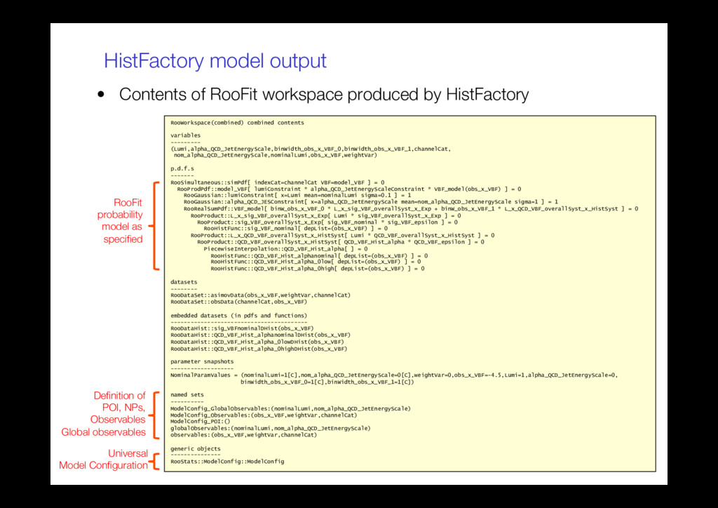
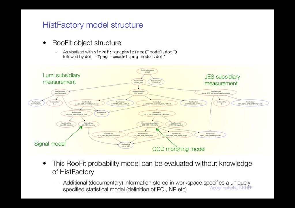
109. HistFactory model output •  Contents of RooFit workspace produced by HistFactory Wouter Verkerke, NIKHEF RooWorkspace(combined) combined contents variables --------- (Lumi,alpha_QCD_JetEnergyScale,binWidth_obs_x_VBF_0,binWidth_obs_x_VBF_1,channelCat, nom_alpha_QCD_JetEnergyScale,nominalLumi,obs_x_VBF,weightVar) p.d.f.s ------- RooSimultaneous::simPdf[ indexCat=channelCat VBF=model_VBF ] = 0 RooProdPdf::model_VBF[ lumiConstraint * alpha_QCD_JetEnergyScaleConstraint * VBF_model(obs_x_VBF) ] = 0 RooGaussian::lumiConstraint[ x=Lumi mean=nominalLumi sigma=0.1 ] = 1 RooGaussian::alpha_QCD_JESConstraint[ x=alpha_QCD_JetEnergyScale mean=nom_alpha_QCD_JetEnergyScale sigma=1 ] = 1 RooRealSumPdf::VBF_model[ binW_obs_x_VBF_0 * L_x_sig_VBF_overallSyst_x_Exp + binW_obs_x_VBF_1 * L_x_QCD_VBF_overallSyst_x_HistSyst ] = 0 RooProduct::L_x_sig_VBF_overallSyst_x_Exp[ Lumi * sig_VBF_overallSyst_x_Exp ] = 0 RooProduct::sig_VBF_overallSyst_x_Exp[ sig_VBF_nominal * sig_VBF_epsilon ] = 0 RooHistFunc::sig_VBF_nominal[ depList=(obs_x_VBF) ] = 0 RooProduct::L_x_QCD_VBF_overallSyst_x_HistSyst[ Lumi * QCD_VBF_overallSyst_x_HistSyst ] = 0 RooProduct::QCD_VBF_overallSyst_x_HistSyst[ QCD_VBF_Hist_alpha * QCD_VBF_epsilon ] = 0 PiecewiseInterpolation::QCD_VBF_Hist_alpha[ ] = 0 RooHistFunc::QCD_VBF_Hist_alphanominal[ depList=(obs_x_VBF) ] = 0 RooHistFunc::QCD_VBF_Hist_alpha_0low[ depList=(obs_x_VBF) ] = 0 RooHistFunc::QCD_VBF_Hist_alpha_0high[ depList=(obs_x_VBF) ] = 0 datasets -------- RooDataSet::asimovData(obs_x_VBF,weightVar,channelCat) RooDataSet::obsData(channelCat,obs_x_VBF) embedded datasets (in pdfs and functions) ----------------------------------------- RooDataHist::sig_VBFnominalDHist(obs_x_VBF) RooDataHist::QCD_VBF_Hist_alphanominalDHist(obs_x_VBF) RooDataHist::QCD_VBF_Hist_alpha_0lowDHist(obs_x_VBF) RooDataHist::QCD_VBF_Hist_alpha_0highDHist(obs_x_VBF) parameter snapshots ------------------- NominalParamValues = (nominalLumi=1[C],nom_alpha_QCD_JetEnergyScale=0[C],weightVar=0,obs_x_VBF=-4.5,Lumi=1,alpha_QCD_JetEnergyScale=0, binWidth_obs_x_VBF_0=1[C],binWidth_obs_x_VBF_1=1[C]) named sets ---------- ModelConfig_GlobalObservables:(nominalLumi,nom_alpha_QCD_JetEnergyScale) ModelConfig_Observables:(obs_x_VBF,weightVar,channelCat) ModelConfig_POI:() globalObservables:(nominalLumi,nom_alpha_QCD_JetEnergyScale) observables:(obs_x_VBF,weightVar,channelCat) generic objects --------------- RooStats::ModelConfig::ModelConfig RooFit! probability! model as ! specified Definition of! POI, NPs,! Observables Global observables! Universal! Model Configuration
110. HistFactory model structure •  RooFit object structure –  As visalized with simPdf::graphVizTree(“model.dot”) followed by dot –Tpng –omodel.png model.dot’ •  This RooFit probability model can be evaluated without knowledge of HistFactory –  Additional (documentary) information stored in workspace specifies a uniquely specified statistical model (definition of POI, NP etc) Wouter Verkerke, NIKHEF JES subsidiary! measurement Lumi subsidiary! measurement QCD morphing model Signal model
111. Make your own Higgs combination •  Workspace technology greatly simplifies combination ! of measurements •  Example: ATLAS Higgs likelihood combination –  Individual channels build likelihood model in workspace file –  A posteriori combine likelihood for each channel in combination group –  Must make sure common parameter have common names, otherwise technically straightforward (in principle) •  Simplified code example –  Real life a bit more complicated, but similar to this concept. Wouter Verkerke, NIKHEF RooWorkspace combined(“combined”) ; // Import channel models from separate workspace files w.importFromFile(“htoZZ.root:w:masterPdfZZ”,…) ; w.importFromFile(“htoWW.root:w:aaronsWWPdf”,…) ; // Create joint pdf w.factory(“SIMUL::joint(index[HWW,HZZ], HZZ=masterPdfZZ,HWW=aaronsWWPdf)”) ;
112. The full ATLAS Higgs combination in a single workspace… F(x,p) x p Atlas Higgs combination model (23.000 functions, 1600 parameters) Model has ~23.000 function objects, ~1600 parameters Reading/writing of full model takes ~4 seconds! ROOT file with workspace is ~6 Mb
113. Collaborative analyses with workspaces •  Workspaces allow to share and modify very complex analyses with very little technical knowledge required •  Example: Higgs coupling fits Wouter Verkerke, NIKHEF Full ! Higgs ! model Signal! strength! in 5! channels Reparam! in terms! of fermion,! v-boson! scale ! factors Confidence! intervals! on Higgs! fermion,! v-boson! couplings
114. Collaborative analyses with workspaces •  How can you reparametrize existing Higgs likelihoods in practice? •  Write functions expressions corresponding to new parameterization •  Edit existing model Wouter Verkerke, NIKHEF RooFormulaVar mu_gg_func(“mu_gg_func”, “(KF2*Kg2)/(0.75*KF2+0.25*KV2)”, KF2,Kg2,KV2) ; w.import(mu_gg_func) ; w.factory(“EDIT::newmodel(model,mu_gg=mu_gg_gunc)”) ; Top node of original Higgs combination pdf Top node of modified Higgs combination pdf Modification prescription replace parameter mu_gg with function mu_gg_func everywhere
115. The role of the RooStats package •  Use of likelihoods so far restricted to parameter, variance estimation and MINOS-style intervals! •  For p-values and Frequentist confidence intervals need to construct (profile likelihood ratio) test statistic and obtain its! (asymptotic distribution)! •  RooStats can do these calculations –  Input is RooWorkspace – contains full likelihood and associated information,! only ‘technical’ tool configuration is needed –  Designed as a toolkit (with classes representing TestStatistics, NeymanConstruction, Intervals, HypothesisTestInverters) –  Very flexible, but usually requires a bit of coding to setup to achieve the desired configuration. Wouter Verkerke, NIKHEF
116. An example of a custom RooStats driver script Tool to calculate p-values for a given hypothesis Tool to construct ! interval from ! hypo test results The test statistic to be used for! the calculation! of p-values ) (µ µ ʹ′ q µ µ µ µ dq q f obs q ∫ ∞ ʹ′ , ) | ( ) | ( µ µ ʹ′ q f Tool to construct! test statistic! distribution
117. The ‘standard’ RooStats driver script •  Input information needed –  Input workspace (file name and workspace name) –  Name of ModelConfig object to be used in workspace •  Specifies S+B model, B model (if not S+B with µ=0), POI, nuisance params etc –  Name of observed dataset in workspace •  Statistics options –  Calculator type (Frequentist, Hybrid, Asymptotic) –  Test statistic (ProfileLR [LHC], RatioOfPLR [TeV], LR [LEP]) –  Use CLS technique (yes/no) •  Technical options –  Range of POI to scan –  Fixed number of steps (for nice plots), ! or -1 for adaptive sampling (for precise and fast limit calculations) Wouter Verkerke, NIKHEF, 117
118. Example output of hypothesis test inversion •  Hypothesis test calculator computes p-value for each value of µ Wouter Verkerke, NIKHEF, 118 HypoTest result (p-value) at given µ (here µ=1) One-sided in interval (upper limit) at 95% C.L. Two-sided in interval at 68% C.L.
119. Summary on RooFit/RooStats/HistFactory •  RooFit is a language to build probability models of arbitrary type, shape and complexity –  Small set of powerful adjustable building blocks simplify building process! (concepts of previous section can all be coded in O(5) lines) –  Concept of ‘workspace’ allows complete separation of process of building and using likelihood models •  HistFactory is a descriptive language for measurements exclusively formulated in template likelihood models –  Declaration of channels, samples and their properties (systematic uncertainties etc) can be turned into a RooFit probability model •  Workspace concept facilitates easy sharing, combining and editing of likelihood functions between analysis groups •  Parameter/Variance estimation and MINOS-style intervals on likelihood models calculated with RooFit/MINUIT tools –  For ‘fundamental methods’ (Frequentist/Bayesian statements) RooStats toolkit can perform calculations based in RooFit models Wouter Verkerke, NIKHEF
120. Wouter Verkerke, NIKHEF Diagnostics II: Overconstraining & choices in modeling ! parametrization 5
121. Role reversal of physics and subsidiary measurements •  As mention in Section 3, full (profile) likelihood treats physics and subsidiary measurement on equal footing •  Our mental picture:! •  Is this picture (always) correct?! ! Wouter Verkerke, NIKHEF L(N,0 | s,!) = Poisson(N | s + b(1+ 0.1!))!Gauss(0 |!,1) Physics measurement Subsidiary measurement “measures s” “measures Ћ” “dependence on Ћ! weakens inference on s”
122. Understanding your model – what constrains your NP •  The answer is no – not always! Your physics measurement! may in some circumstances constrain Ћ better than your subsidiary measurement. •  Doesn’t happen in Poisson counting example –  Physics likelihood has no information to distinguish effect of s from effect of α •  But if physics measurement is based on a distribution or comprises multiple distributions this is well possible Wouter Verkerke, NIKHEF L(N,0 | s,!) = Poisson(N | s + b(1+ 0.1!))!Gauss(0 |!,1) Physics measurement Subsidiary measurement
123. Understanding your model – what constrains your NP •  A case study – measuring jet multiplicity –  Physics observable of interest is a jet multiplicity spectrum ! [3j,4j,5j] after an (unspecified) pT cut. –  Describe data with sum of signal (mildly peaking at 4j) and ! a single background (exponentially falling in nj). –  POI is signal strength modifier µ. –  Jet Energy Scale is the leading ! systematic uncertainty •  JES strongly affects jet multiplicity ! after a pT cut, •  Effect modeled by response ! function rs (α) •  Magnitude of uncertainty on α ! constrained by subsidiary ! measurement Wouter Verkerke, NIKHEF L( ! N | µ,!JES ) = Poisson( i=3,4,5 ! N i |(µ " ! s i "+ ! b i )"r s (!JES )))"Gauss(0 |!JES ,1)
124. Understanding your model – what constrains your NP •  Now measure (Ж,Ћ) from data – 80 events! •  Is this fit OK? –  Effect of JES uncertainty propagated in to µ via response modeling in likelihood. Increases total uncertainty by about a factor of 2 –  Estimated uncertainty on α is not precisely 1, as one would expect! from unit Gaussian subsidiary measurement… Wouter Verkerke, NIKHEF ˆ µ =1.0 ± 0.37 ˆ ! = 0.01± 0.83 Estimators of! Ж, Ћ correlated! due to similar! response in physics! measurement Uncertainty! on Ж without effect of JES
125. Understanding your model – what constrains your NP •  The next year – 10x more data (800 events)! repeat measurement with same model •  Is this fit OK? –  Uncertainty of JES NP much reduced w.r.t. subsidiary meas. (α = 0 ± 1) –  Because the physics likelihood can measure it better than the subsidiary measurement (the effect of µ, α are sufficiently distinct that both can be constrained at high precision) Wouter Verkerke, NIKHEF ˆ µ = 0.90 ± 0.13 ˆ ! = !0.23± 0.31 Estimators of! Ж, Ћ correlated! due to similar! response in physics! measurement
126. Understanding your model – what constrains your NP •  Is it OK if the physics measurement constrains NP associated with a systematic uncertainty better than the designated subsidiary measurement? –  From the statisticians point of view: no problem, simply a product of two likelihood that are treated on equal footing ‘simultaneous measurement’ –  From physicists point of view? Measurement is only valid is model is valid. •  Is the probability model of the physics measurement valid? •  Reasons for concern –  Incomplete modeling of systematic uncertainties, –  Or more generally, model insufficiently detailed Wouter Verkerke, NIKHEF L( ! N | µ,!JES ) = Poisson( i=3,4,5 ! N i |(µ " ! s i "+ ! b i )"r s (!JES )))"Gauss(0 |!JES ,1)
127. Understanding your model – what constrains your NP •  What did we overlook in the example model? –  The background rate has no uncertainty! –  Insert modeling of background uncertainty! ! •  With improved model! accuracy estimated! uncertainty on both! ЋJES , Ж goes up again… –  Inference weakened! by new degree of! freedom αbkg –  NB αJES estimate still! deviates a bit from normal! distribution estimate… Wouter Verkerke, NIKHEF L( ! N | µ,!JES ,!bkg ) = Poisson( i=3,4,5 ! N i |(µ " ! s i "+ ! b i "r b (!bkg ))"r s (!JES )))"Gauss(0 |!JES ,1)"Gauss(0 |!bkg ,1) Background rate! subsidiary measurement Background rate! response function ˆ µ = 0.93± 0.29 ˆ !JES = 0.90 ± 0.70 ( ˆ !bkg =1.36 ± 0.20)
128. Understanding your model – what constrains your NP •  Lesson learned: if probability model of a physics measurement is insufficiently detailed (i.e. flexible) you can underestimate uncertainties •  Normalized subsidiary measurement provide an excellent diagnostic tool –  Whenever estimates of a NP associated with unit Gaussian subsidiary measurement deviate from α = 0 ± 1then physics measurement is constraining or biases this NP. –  Always inspect all NPs of your fit for such signs! •  Is ‘over-constraining’ of systematics NPs always bad? –  No, sometimes there are good arguments why a physics measurement can measure a systematic uncertainty better than a dedicated calibration measurement (that is represented by the subsidiary measurement) –  Example: in sample of reconstructed hadronic top quarks tàbW(qq), the pair of light jets should always have m(jj)=mW. For this special sample of jets it will possible to calibrate the JES better than with generic calibration measurement Wouter Verkerke, NIKHEF
129. Commonly heard arguments in discussion on over-constraining •  Overconstraining of a certain systematic is OK “because this is what the data tell us” –  It is what the data tells you under the hypothesis that your model is correct. The problem is usually in the latter condition •  “The parameter ЋJES should not be interpreted as Jet Energy Scale uncertainty provided by the jet calibration group” –  A systematic uncertainty is always combination of response prescription and one or more nuisance parameters uncertainties. –  If you implement the response prescription of the systematic, then the NP in your model really is the same as the prescriptions uncertainty •  “My estimate of ЋJES = 0 ± 0.4 doesn’t mean that the ‘real’ Jet Energy Scale systematic is reduced from 5% to 2% –  It certainly means that in your analysis a 2% JES uncertainty is propagated to the POI instead of the “official” 5%. –  One can argue that the 5% shouldn’t apply because your sample is special and can be calibrated better by a clever model, but this is a physics argument that should be documented with evidence for that (e.g. argument JES in tàbW(qq) decays) Wouter Verkerke, NIKHEF
130. Dealing with over-constrained systematic NPs •  Step 1 – Diagnostics –  Always inspect nuisance parameters in your fit for signs of over-constraining •  Step 2 – Analyze –  Are there systematic uncertainties overlooked in the construction of the likelihood that introduce unwarranted physics assumption in model that ML estimator exploits to constrain models? –  Is your systematic uncertainty conceptually covered by a single nuisance parameter? do you perhaps need more NPs? –  In case the physics likelihood comprises multiple samples, do you assume fully correlated responses functions, whereas sample composition should conceptually allow for some degree of decorrelation? •  Step 3 – Solution –  If over-constraining is analyzed to be the result of inaccurate modeling, improve model structure, add new NPs, decompose NPs in different ways to reflect sample correlations –  If constraint from physics is believed to be document studies as part of your physics analysis Wouter Verkerke, NIKHEF
131. Dealing with over-constraining – introducing more NPs •  Some systematic uncertainties are not captured well by one nuisance parameter. •  Example Jet Energy Scale –  Statement “the JES uncertainty is 5% for all jets” does not necessarily imply that the calibration of all jets can be modeled with a single NP. –  A single NP implies that the calibration can only be coherently off among all jets. Such an assumption allows, for example, to precisely constrain JES with a high-statistics sample of low-pT jets, and then transport that reduced uncertainty to high-pT jets, using the calibration scale coherency encoded in the model –  In reality correlation between the energy scale of low-pT and high-pT jets is controlled by the detector design and calibration procedure and is likely a lot more complicated à Invalid modeling of systematic uncertainties often a result of ‘own interpretation’ of imprecisely formulated systematic prescription. –  Besides this, a calibration may have multiple sources of uncertainty that were lumped together in a prescription (calibration measurements, simulation assumptions, sample-dependent effects) that would need to be individually modeled Wouter Verkerke, NIKHEF
132. Dealing with over-constraining – Theory uncertainties •  Over-constraining of theory uncertainties in physics measurements has different set of issues than for detector uncertainties •  Different: In principle it is the goal of physics measurements to constrain theory uncertainties –  So role of physics measurement and subsidiary measurement are not symmetric: the latter quantifies some ‘degree of belief’ that is not based on an experimental measurement. –  Likelihood of physics measurement constitutes an experimental measurement and is in principle preferred over ‘belief’ –  But question remains if physics likelihood was well designed to constrain this particular theory uncertainty. •  Same: response function and set of NPs must be able to accurately capture underlying systematic effect. –  Sometimes easy, e.g. ‘renormalization scale’ has well-defined meaning in a given theoretical model and a clearly identifiable single associated parameter –  Sometimes hard, e.g. ‘Pythia vs Herwig’. Not clear what it means or how many degrees of freedom underlying model has. Wouter Verkerke, NIKHEF
133. Dealing with ‘two-point’ uncertainties •  In discussion of rate systematics in Section 3 ! it was mentioned that ‘two-point systematics’ ! can always be effectively represented with an ! interpolation strategy! ! •  But this argument relies crucially on the dimensional correspondence between the observable and the NP –  The effect on a scalar observable can always be modeled with one NP –  In other words the existence of a 3rd generator ‘Sherpa’ can always be! effectively capture by the Pythia-Herwig inter/extrapolation –  It can of course modify your subsidiary measurement (e.g. lending more credence to the Pythia outcome if its result is close, but response model is still valid) Wouter Verkerke, NIKHEF Ћgen b Background rate Nuisance parameter Pythia Herwig Response model Subsidiary meas.
134. Dealing with ‘two-point’ uncertainties •  If ‘2-point’response functions models a distribution, the response corresponding to a new ‘third point’ is not necessarily mapped by b(Ћ) for any value of Ћ •  This point is important in the discussion to what extent a two- point response function can be over-constrained. –  A result α2p = 0.5 ± 1 has ‘reasonable’ odds to cover the ‘true generator’ assuming all generators are normally scattered in an imaginary ‘generator space’ Wouter Verkerke, NIKHEF Pythia Herwig Sherpa Nature Next years! generator Modeled uncertainty (1 dimension)! assuming ‘nature is on line’ Effectively captured uncertainty! ! under the assumption that effect! of ‘position in model space’ in ! any dimension is similar on! response function
135. Dealing with ‘two-point’ uncertainties •  If ‘2-point’response functions models a distribution, the response corresponding to a new ‘third point’ is not necessarily mapped by b(Ћ) for any value of Ћ •  This point is important in the discussion to what extent a two- point response function can be over-constrained. –  Does a hypothetical overconstrained result α2p = 0.1 ± 0.2 ‘reasonably’ cover the generator model space? Wouter Verkerke, NIKHEF Pythia Herwig Sherpa Nature Next years! generator Modeled uncertainty (1 dimension)! assuming ‘nature’ is on line Effectively captured uncertainty! ! under the assumption that effect! of ‘position in model space’ in ! any dimension is similar on! response function
136. Dealing with ‘two-point’ uncertainties •  Arguments on representativeness of sampling points of ‘2 point’ models raise questions in validity of physics models that over-constrain these •  The main problem is that you become rather sensitive to things you don’t know and quantify: the ‘dimensionality’ of the generator space. –  To understand what you are doing you’d need to know what all degrees of freedom are (and ideally what they conceptually represent) –  Unless you know this – trying to reduce the ‘considered space of possibilities’ is rather speculative –  The real problem is often that you don’t really know what causes the ‘Pythia/Herwig’ effect. Unless you learn more about that there is no real progress. •  The ‘unknown dimensionality’ problem often enters a model in a seemlingly standard modeling assumptions –  Take an inclusive cross-section measurement –  Needs to extrapolate acceptance region! to full inclusive phase space using generator! à Introduces generator systematic –  Physics likelihood can ‘measure’ ! that nature inside acceptance is very ! Pythia-like insideusing 2-point ! response function with 1 NP –  Is nature in the entire phase space therefore! Pythia-like? If yes, we can greatly reduce! inclusive cross-section uncertainty, if no, not… Generator phase space Analysis acceptance Nature! is measured! to be very! Pythia-like! here Is nature! therefore! also very Pythia-like! here?
137. Ad-hoc solutions - decorrelation •  NPs that are determined to overconstrained due to incorrect modeling assumption can be eliminated through the process of ad-hoc decorrelation •  Take two-bin simple Poisson counting model and a single systematic uncertainty that is modeled in both bins ! –  The physics part of this likelihood may over-constrain α if ! effect of changing µ or α has a different effect on (NA ,NB ) –  Can eliminate overconstraint due to correlation between A and B samples by introducing separate NPs for A and B sample –  Interpretation: e.g. for JES, effectively independent calibrations due to different sample composition (e.g. different pT spectra) –  Note that some physics POIs are sensitive to ratios of yields, in such cases a correlated NP may be the more conservative choice Wouter Verkerke, NIKHEF L(N A , N B | µ,!) = P(N A |(µ ! ! s A + ! b A )!r A (!))! P(N B |(µ ! ! s B + ! b B )!r B (!))!G(0 |!,1) L(N A , N B | µ,!A ,!B ) = P(N A |(µ ! ! s A + ! b A )!r A (!A ))! P(N B |(µ ! ! s B + ! b B )!r B (!B ))!G(0 |!A ,1)!G(0 |!B ,1) Ж! sA Ж sB bA bB A B A B
138. Ad-hoc solutions – Decorrelation •  Another common type of likelihood model prone to overconstraining issues is the ‘signal/control region model’! –  Control regions measures background rate in CR,! mapped background rate is SR via transport factor r(a) –  Signal in SR modeled from MC simulation •  Both signal acceptance and background transport! factor depend on simulation and are subject to ! systematic uncertainties –  Common solution à coherent modeling of response functions e.g. for JES –  But transport factor sensitive to ratio of JES response in CR and SR, signal modeling to JES response in SR only. –  Since measurement of ‘A/B and B’ is equivalent to measurement of A and B physics likelihood can still over-constrain single JES NP from such a model –  Solution: decorrelate JES for signal model and transport factor Wouter Verkerke, NIKHEF L(N SR , N CR | b,µ,!) = P(N SR |(µ ! ! s !r s (!)+ b!r trams (!))! P(N CR | b)!G(0 |!,1) Ж! sA b b! r (Ћ) SR CR r(Ћ)
139. Summary •  When performing profile likelihood fits –  Diagnose carefully if NPs associated with systematic uncertainties are! (over)constrained by physics measurements –  For overconstrained NPs, assess correctness of response model, and choice of sufficient number of NPs to describe underlying systematic uncertainty –  If overconstraining can be justified on physics arguments, document this as part of the analysis –  If overconstraining cannot be justified, upgrade to improved response model, or perform ad-hoc decorrelations if that is not possible –  Use your physics judgement – focus on modeling problems that matter for your POI •  For ‘irrelevant’ NPs (i.e. those that correlate weakly to your POI) overconstraining may be a non- issue, on the other hand, de-correlation of such NPs will not adversely affect your result and simply analysis approval discussions. Wouter Verkerke, NIKHEF
140. Summary •  Diagnostics over NP overconstraining provide powerful insight into your analysis model –  An overconstrained NP indicates an externally provided systematic is inconsistent with physics measurement –  This may point to either an incorrect response modeling of that uncertainty, to result in a genuinely better estimate of the uncertainty –  Solution not always clear-cut, but you should be at least aware of it. –  Note that over-constraining always points to an underlying physics issue! (lack of knowledge, simplistic modeling) à Treat it as a physics analysis problem, not as a statistics problem •  Diagnostic power of profile likelihood models highlights one of the major shortcomings of the ‘naïve’ strategy of error propagation (as discussed in Section 1) –  Physics measurement can entangle in non-trivial ways with systematic uncertainties Wouter Verkerke, NIKHEF
141. Example of likelihood modeling diagnostics Wouter Verkerke, NIKHEF
142. Wouter Verkerke, NIKHEF Summary! & conclusions 6
143. Summary •  Modelling of systematic uncertainties in the likelihood (‘profiling’) ! is the best we know to incorporate systematic uncertainties in rigorous statistical procedures –  Profiling requires more a ‘exact’ specification of what a systematic uncertainty means that traditional prescritions à this is good thing, it makes you think about (otherwise hidden) assumption –  It’s important to involve the ‘author’ of uncertainty prescription in this process, as flawed assumptions can be exploited by statistical methods to arrive at unwarranted conclusions –  Systematic uncertainties that have conceptual fuzziness (‘pythia-vs-herwig’)! are difficult to capture in the likelihood, but this is a reflection of an underlying physics problem –  Good software tools exist to simplify the process of likelihood modeling –  It’s important to carefully diagnose your profile likelihood models for both technical and interpretational problems (‘over-constraining’) Wouter Verkerke, NIKHEF