Fish Schooling investigated by using IB-LBM

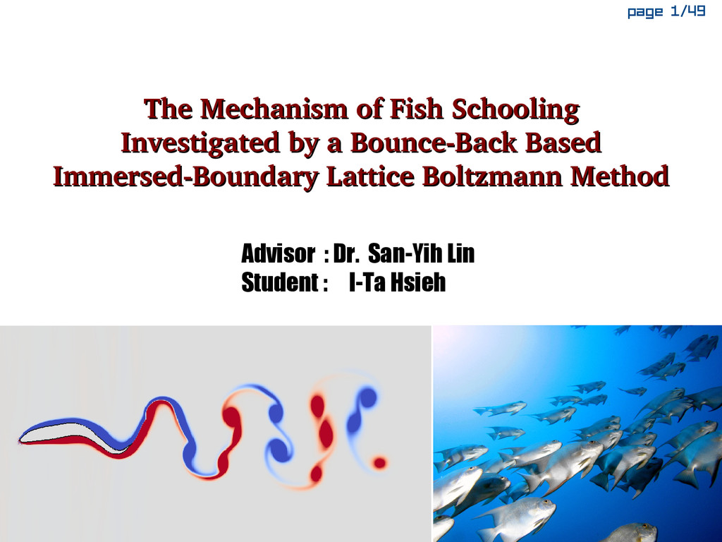
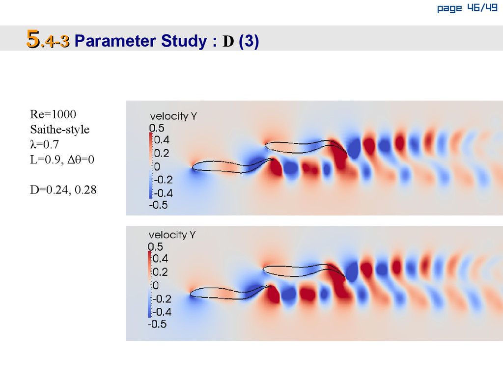
To study the problem whether there is any hydrodynamical function in fish schooling, an bounce-back based immersed-boundary lattice Boltzmann method was developed to cope with the moving boundary problem. A method to decompose the force into shear and normal force by momentum exchange in lattice Boltzmann method is provided. This algorithm performs as well as the accuracy of the theoretical analysis in stationary-boundary test, and the characteristics of the non-dimensional relaxation time τ is also discovered. In low Reynolds number flow, the results by the current method are comparable to the former experiments. Under the proposed numerical scheme, in two-dimensional fish schooling we proposed a new mechanism that infers the following fish just find the best place to follow by, instead of to arrange themselves in the regular position.

Transcript

1. page 1/49 The Mechanism of Fish Schooling The Mechanism of Fish Schooling Investigated by a Bounce­Back Based Investigated by a Bounce­Back Based Immersed­Boundary Lattice Boltzmann Method Immersed­Boundary Lattice Boltzmann Method Advisor : Dr. San-Yih Lin Student : I-Ta Hsieh
2. page 2/49 Outline 1. Literature Review 2. Theory of Lattice Boltzmann Method 3. The Bounce-back based IB-LBM 4. Numerical Test 5. Swimming-Fish Simulation 6. Conclusion
3. page 3/49 Literature Review ▪Aquatic Animal Locomotion 1. “Flying and swimming animals cruise at a Strouhal number tuned for high power efficiency,” Taylor, Nudds, and Thomas. (2003) 2. “Review of fish swimming modes for aquatic locomotion,” Sfakiotakis, Lane, and Davies. (1999) 3. “Hydrodynamics of fish schooling,” Weihs (1973) ▪Lattice Boltzmann Method 1. “A note on the lattice Boltzmann method beyond the Chapman-Enskog limits,” Sbragaglia and Succi. (2006) 2. “The mathematical theory of non-uniform gases,” Chapman and Cowling.
4. page 4/49 Literature Review - The Schooling Mechanism Mentioned by Weihs (1973) Channeling hypothesis (anti-phase) Vortex hypothesis (inphase)
5. page 5/49 2.1 Brief History of LBM 2.2 Overview of LBM 2.3 Equilibrium Distribution Function 2.4 Kinetic Limit 2.5 The Technique of Chapman-Enskog Expansion Theory of Lattice Boltzmann Method
6. page 6/49 2 2.1 .1 Brief History of Lattice Boltzmann Method Ludwig Boltzmann(1844-1906) Boltzmann equation in Stosszahl Ansatz. ∂ f ∂t V⋅ ∂ f ∂ x F⋅ ∂ f ∂ v = ∣ coll ∣ coll = ∬ g p− p' ,q[ f  pq f  p'−q− f  p f  p' ]d p' d q David Enskog(1884-1947) "Kinetic theory of the processes in moderately dilute gases"(1917) Bhatnagar,Gross,and Krook(1954) BGK collision model ∣ coll = − f x ,v ,t− f eq x ,v ,t v Broadwell(1964) Molecules move in six discrete velocity(Lattice Gas Cellular Automata) Frisch,Hasslacher,and Pomeau(1986) Lattice Boltzmann equation implement in FHP
7. page 7/49 f i (x+e i Δt ,t+Δt) = f i (x ,t) − 1 τ [ f i (x ,t)− f i eq(x ,t)] ⇒ {collision process , ̃ f i (x ,t) = f i (x ,t) − 1 τ [ f i (x ,t)− f i eq(x ,t)] streaming process , f (x+e i Δt ,t+Δt) = ̃ f i (x ,t) Density ρ=Σ f i , Momentum ρu=Σ f i e i , Kinematic viscosity ν = 2τ−1 6 c2 Δt 1 2 3 4 5 6 7 8 D2Q9 grid model Bhatnagar-Gross-Krook(BGK) Lattice Boltzmann Equation 0 Equilibrium distribution function f i eq = ρw i [1+ 3 c2 (e i ⋅u)+ 9 2c4 (e i ⋅u)2− 3 2c2 u2] weighting function w i = {4 9 , i=0 1 9 , i=1,2,3,4 1 36 , i=5,6,7,8 thermodynamic speed c= Δ x Δt = √3c s 2 2.2 .2 Overview of Lattice Boltzmann method
8. page 8/49 Calculate maximum entropy defined by Boltzmann S = k ln w Assume total N particles distribute at e i discrete velocity state. It leads to Maxwell-Boltzmann distribution function while N is large enough. N (e i ) = α⋅eβ(e i −u)2 From conservation of particle number and applying Equipartition theorem for two-dimensional monoatomic dilute gas. We get α=N m 2π kT , β= −m 2 kT Use four Guassian quadrature integrals and solve. w i = {4 9 , i=0 1 9 , i=1,2,3,4 1 36 , i=5,6,7,8 , c2= 3 kT m =3c s 2 c s is speed of sound in ideal gas Expand eβ(u2−2u⋅e i ) by Taylor series for finite u (low Mach number) and normalize N i to density. Finally we get f eq = w i ρ(1+3e i ⋅u+ 9 2 (e i ⋅u)2− 1 2 u2) 2 2.3 .3 Equilibrium Distribution Function
9. page 9/49 BGK's collision model can be stated as d f i (⃗ x ,t) dt = ∂ f i (⃗ x ,t) ∂t +⃗ e i ⋅⃗ ∇ f i (⃗ x ,t) = −ω[ f i (⃗ x ,t)− f i eq (⃗ x ,t)] ω is average collision frequency Integral from t to t+Δt with the "survival function." BE becomes to f t+Δt = e−ω Δt f t + (eD Δt−e−ω Δt 1+ D ω )f t eq , D is differential operator. Neglect the equilibrium variation on scale Δt ⇒ D=0 f t+Δt = e−ω Δt f t +(1−e−ωΔt ) f t eq , (Lattice Boltzmann slution) 2 2.4 .4 Kinetic Limit (1) – based on Sbragaglia and Succi
10. page 10/49 Error ≈ eKn−Kn21−e −1 Kn  eKn−e −1 Kn  = 1 1−e− t Asyptotic relaxation time =0.5Kn ⇒ Kn = 3 c2  t which agrees with Inamuro et. al.'s result(1997) 2 2.4 .4 Kinetic Limit (2) – based on Sbragaglia and Succi
11. page 11/49 As Enskog's three assumption : 1. f can be expanded as f = f (0)+ f (1)+ f (2)+⋯ (infinite terms) 2. There exits a function ξ( f )=0 , and ξ( f ) can be expand as ξ( f ) = ξ(0)( f (0))+ξ(1) ( f (0) , f (1))+ξ(2)( f (0) , f (1) , f (2))+⋯ (infinite functions) 3. ξ( f ) =0 has a simple solution. That is, for each ξ(n)( f (0) ,⋯, f (n))=0 Let ξ( f )= f t+Δt − f t + 1 τ [ f t − f t eq ] (i.e. LBE) Expand f for only three terms. Finally it will approach Navier-Stokes eqution. ρ ∂u j ∂t +ρu k ∂u j ∂ x k = ∂ ∂ x k {−P δij +(τ− 1 2 )Δt [1 3 ρ c2 (∂u j ∂u k + ∂u k ∂ u j )− ∂ ∂ x l u j u k u l ]}+Ο[(τ− 1 2 )Δt] 2 2 2.5 .5 The Technique of Chapman-Enskog Expansion (1)
12. page 12/49 We obtain kinematic viscocity ν= 2 τ−1 6 c2 Δt and the term − ∂ ∂ x l u j u k u l goes against Galilean invariant Furthermore, Qian and Zhou(1998) have given a modification of it.  in the well-known Chapman-Enskog expansion have two kinds of implication. f = f 0 f 12 f 2⋯ 1. Represent an infitisimal Knudsen number Kn in physics. 2. =1 would satisfy Enskog's assumption. 2 2.5 .5 The Technique of Chapman-Enskog Expansion (2)
13. page 13/49 3.1 The Bounce-Back Based Immersed Boundary 3.2 The Algorithm of IB-LBM 3.3 Force Evaluation The Bounce-Back Based IB-LBM
14. page 14/49 Generalize the instruction on IB. f t+Δt = {f i (⃗ x+⃗ e i Δt) = f i − 1 τ ( f i − f eq) streaming out f i (⃗ x) = f ̄ i +2⋅3 w i ρ⃗ u⋅⃗ e i bounce back , ϕ(⃗ x+⃗ e i Δt)=0 f i (⃗ x) = f i − 1 τ ( f i − f eq) collision only , (ϕ(⃗ x+⃗ e i Δt)=1)∧(ϕ(⃗ x−⃗ e i Δt)=1) The moving boundary problem requires its corresponding pressure boundary condition. It is important especially for a propulsion system because the thrust is always contributed by pressure force. Consider about 3 prototypes of IB boundary flat convex concave 3 3.1 .1 The Bounce-Back based Immersed-Boundary
15. page 15/49 1. Set preferred IB-phase function and the velocity on the boundary. 2. Determine the wall of IB. 3. Collision and streaming of the flow field. 4. Collision and streaming from wall to the flow field, and go on to bounce back and momentum exchange. Only collision in other direction. Downwind-direction determination on wall. 5. Macroscopic variable evaluation. 6. Boundary condition 7. Correct the density inside IB with the downwind-direction side from the wall. Reset the distribution function to equilibrium. 8. Go time iteration 3 3.2 .2 The Algorithm of IB-LBM
16. page 16/49 1. Momentum exchange ⃗ F = ∑ ϕ=1 ∑ i=1 q {[ f i (⃗ x)+ f ̄ i (⃗ x+⃗ e i Δt)][1−ϕ(⃗ x+⃗ e i Δt)] +[ f i (⃗ x ,t−Δt)− f i (⃗ x ,t)]ϕ(⃗ x+⃗ e i Δt)⋅ϕ(⃗ x−⃗ e i Δt)}⃗ e i Δ x2 Δt F x is {Normal , ϕ(x−e x , y+e y )=1 Shear , ϕ(x−e x , y+e y )=0 F y is {Normal , ϕ(x+e x , y−e y )=1 Shear , ϕ( x+e x , y−e y )=0 2. Volume integral for compressible flow F x = ∑ ϕ=1 [− ∂ P ∂ x +2μ ∂2 u ∂ x2 + μ( ∂2 u ∂ y2 + ∂2 v ∂ x∂ y ) ]Δ x2 F y = ∑ ϕ=1 [− ∂ P ∂ y +2μ ∂2 v ∂ y2 ⏟ Normal force + μ( ∂2 v ∂ x2 + ∂2 u ∂ x ∂ y ) ⏟ shear force ]Δ x2 3. Volume integral used in pressure-based LBM for incompressible flow ⃗ F = ∑ ϕ=1 [−∇ P+∇2 ⃗ u]Δ x2 3 3.3 .3 Force Evaluation
17. page 17/49 4.1 The Stability of LBM and Order Analysis 4.2 Stationary-Body Examination 4.3 Moving-Body Examination 4.4 Oscillatory Motion of an Airfoil 4.5 Traveling-Wavy Foil Numerical Test
18. page 18/49 The best-solving τ in the problem is 1.1 The order of accuracy is about 2. This result agrees with Inamuro et. al. (1997) 4 4.1.1 .1.1 Formation of Couette Flow
19. page 19/49 The best-solving τ in the problem is 1.2 The order of accuracy is about 3.4 4 4.1.2 .1.2 Stokes' Second Problem
20. page 20/49 4 4.2 .2 Flow over a Circular Cylinder (1)
21. page 21/49 4 4.2 .2 Flow over a Circular Cylinder (2)
22. page 22/49 4 4.2 .2 Flow over a Circular Cylinder (3)
23. page 23/49 4 4.2 .2 Flow over a Circular Cylinder (4)
24. page 24/49 4 4.2 .2 Flow over a Circular Cylinder (5)
25. page 25/49 4 4.3 .3 An Accelerating Pitching Airfoil
26. page 26/49 +=0.5 +=2.4
27. page 27/49 Strouhal number = f L U ∞ , L is trasverse characteristic length Reduced frequency = c 2U ∞ Plunging Airfoil Pitching Airfoil Fish-like Motion L = 2hc h is the ratio of the amplitude and the chord. L = 2c  is the amplitude of the pitching AOA St = 2kh  St = 2k   St = f *  L = A,  = A c 4 4.4­1 .4­1 The Definition of Strouhal number
28. page 28/49 4 4.4­2 .4­2 An Oscillatory Pitching Airfoil
29. page 29/49 Re=100 h=0.1 k=3.0, 3.5, 4.0, 4.5, 4 4.4­3 .4­3 A Plunging Airfoil in the Wind Tunnel
30. page 30/49 Cartesian cell-cut method by Chung Re=200 Bounce-Back based IB-LBM Cartesian cell-cut method by Chung Re=2000 Bounce-Back based IB-LBM 4 4.5­1 .5­1 Undulatory Fish Motion Re= ρl2 μT
31. page 31/49 4 4.5­2 .5­2 Wassersug & Hoff's Tadpole (1) Re=3000 Tadpole-style f =0.8, 1.2, 1.4
32. page 32/49 4 4.5­2 .5­2 Wassersug & Hoff's Tadpole (2)
33. page 33/49 4 4.5­3 .5­3 The Decompositions of Drag versus Frequency
34. page 34/49 5.1 Power Consumption and the Efficiency 5.2 The Secant Shooting Method for Equilibrium Finding 5.3 The Optimization of Single-Swimming Fish 5.4 The Mechanism of Fish Schooling Swimming-Fish Simulation
35. page 35/49 Force per unit length along chord ⃗ F given (x)+⃗ F Hydro (x) = m(x)⃗ a(x) Power P = ∫ 0 l ⃗ F given ⋅⃗ V dx = ∫ 0 l (m⃗ a− ⃗ F Hydro )⋅⃗ V dx = ∫ 0 l m⃗ a⋅⃗ V dx−∫ 0 l ⃗ F Hydro ⋅⃗ V dx = ∫ 0 l m d ⃗ V 2 dt dx−∫ 0 l LV dx Take average ̄ P = ∫ 0 l m d ⃗ V 2 dt dx−∫ 0 l LV dx Froude efficiency ηF = ̄ T⋅V ∞ ̄ P = C T C P Coefficient of Power C P = ̄ P 1 2 ρV ∞ 3 l Coefficient of Thrust C T = D 0 − ̄ D 1 2 ρV ∞ 2 l 5 5.1 .1 The Definition of Power Consumption and Efficiency
36. page 36/49 f n+1= f n−C d n× f n− f n−1 C d n−C d n−1 5 5.2 .2 The Secant Shooting Method for Equilibrium Finding f n+1
37. page 37/49 5 5.3 .3 The Optimization of Single-Swimming Fish
38. page 38/49 Re=1000 saithe-style λ=0.6, 0.7, 0.8, 0.9
39. page 39/49 L D Δθe =2π( L λ ) 5 5.4 .4 The Follow-the-Leader mechanism
40. page 40/49 5 5.4­1 .4­1 Parameter Study : Δθ (1)
41. page 41/49 5 5.4­1 .4­1 Parameter Study : Δθ (2) Re=1000 Saithe-style λ=0.7 L=0.9, D=0.3 Δθ=0, 0.7×(2π)
42. page 42/49 5 5.4­2 .4­2 Parameter Study : L (1)
43. page 43/49 5 5.4­2 .4­2 Parameter Study : L (2) Re=1000 Saithe-style λ=0.7 D=0.3, Δθ=0 L=0.7, 0.9
44. page 44/49 5 5.4­3 .4­3 Parameter Study : D (1)
45. page 45/49 5 5.4­3 .4­3 Parameter Study : D (2) Re=1000 Saithe-style λ=0.7 L=0.9, Δθ=0 D=0.24, 0.28
46. page 46/49 5 5.4­3 .4­3 Parameter Study : D (3) Re=1000 Saithe-style λ=0.7 L=0.9, Δθ=0 D=0.24, 0.28
47. page 47/49 6 6.1 .1 Conclusion about the IB-LBM 1. In the stationary boundary test, the IB-LBM achieve second order accuracy as the theoretical analysis. The best solving non- dimensional relaxation time τ probably lies in 1.0 to 1.5 in most of the cases. 2. Single-relaxation time is suitable for low Reynolds number flow or so-called mesoscopic scale, at which 10-2<Kn<101. 3. Non-body-fitted approach method is difficult to capture the sharp edge. In IB-LBM, we recommend a tolerant vale ε to overcome the problem. In spite of losing some accuracy on the body surface, this method inherits the native profit of LBM, easy to implement and potential to be parallelized. 4. The proposed method for decomposing the force has the concrete physical meaning and can be combine into the IB algorithm.
48. page 48/49 (i) The rear fish will synchronize its tail-beat as the lateral velocity of the leading fish's wake to reduce its power consumption. (ii) The two, frontal and rear, fishes will compromise their longitudinal distance to achieve the optimized total efficiency or total shear drag. (iii) The rear fish will adjust the relatively lateral distance to meet its maximum efficiency. 6 6.2 .2 Conclusion about the Fish Schooling The best total efficiency for two swimming fishes in the test is about 59%, which saves about 17% energy compared with single swimming efficiency 49%. It's consistent with Magnusen's estimation, which is between 10% to 20%.
49. page 49/49 Thank You for Listening