Bayesian methods for constraining initial conditions and viscosity

Presented at the 2015 RHIC & AGS Annual Users' Meeting https://www.bnl.gov/aum2015

Transcript

1. Bayesian methods for constraining initial conditions and viscosity Jonah Bernhard (Duke University) 2015 RHIC & AGS Annual Users’ Meeting Tuesday, June 9 J. E. Bernhard, P. W. Marcy, C. E. Coleman-Smith, S. Huzurbazar, R. L. Wolpert, and S. A. Bass, PRC 91, 054910 (2015), arXiv:1502.00339 [nucl-th].
2. Model-to-data comparison | < 1) lab η (| ch N 50 100 150 200 c < 3.0 GeV/ T p < | > 1.4} η ∆ {2, | 2 v {4} 2 v = 5.02 TeV NN s ICE p-Pb | < 1) lab η (| ch N 10 2 10 3 10 2 v 0 0.02 0.04 0.06 0.08 0.1 0.12 | > 1.4} η ∆ {2, | 2 v {4} 2 v {6} 2 v 82 65 52 43 31 17 7 Centrality (%) c < 3.0 GeV/ T p 0.2 < = 2.76 TeV NN s ALICE Pb-Pb Model Initial conditions, τ0, η/s, . . . 0 2000 4000 6000 Glauber ­ Nch ® 0.00 0.04 0.08 0.12 v2 {2} 0.00 0.02 0.04 v3 {2} 0 10 20 30 40 50 Centrality % 0 2000 4000 6000 KLN 0 10 20 30 40 50 Centrality % 0.00 0.04 0.08 0.12 0 10 20 30 40 50 Centrality % 0.00 0.02 0.04 Jonah Bernhard (Duke) Bayesian methods for constraining initial conditions and viscosity 1 / 17
3. Measuring QGP η/s 1. Observe experimental flow coefficients vn 2. Run model with variable η/s 3. Constrain η/s by matching vn 0 10 20 30 (1/S) dN ch /dy (fm-2 ) 0 0.05 0.1 0.15 0.2 0.25 v 2 /ε 0 10 20 30 40 (1/S) dN ch /dy (fm-2 ) hydro (η/s) + UrQMD hydro (η/s) + UrQMD MC-Glauber MC-KLN 0.0 0.08 0.16 0.24 0.0 0.08 0.16 0.24 η/s η/s v 2 {2} / 〈ε2 part 〉1/2 Gl (a) (b) 〈v 2 〉 / 〈ε part 〉 Gl v 2 {2} / 〈ε2 part 〉1/2 KLN 〈v 2 〉 / 〈ε part 〉 KLN H. Song, S. A. Bass, U. Heinz, T. Hirano, and C. Shen, PRL 106, 192301 (2011), arXiv:1011.2783 [nucl-th]. Jonah Bernhard (Duke) Bayesian methods for constraining initial conditions and viscosity 2 / 17
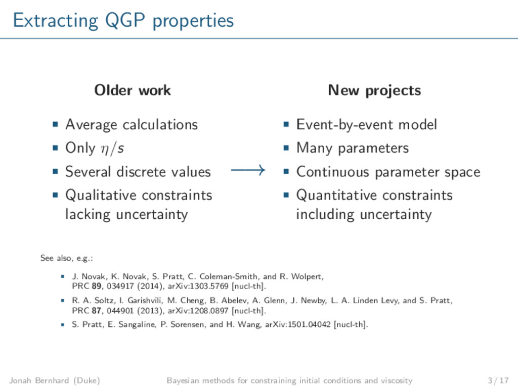
4. Extracting QGP properties Older work Average calculations Only η/s Several discrete values Qualitative constraints lacking uncertainty New projects Event-by-event model Many parameters Continuous parameter space Quantitative constraints including uncertainty See also, e.g.: J. Novak, K. Novak, S. Pratt, C. Coleman-Smith, and R. Wolpert, PRC 89, 034917 (2014), arXiv:1303.5769 [nucl-th]. R. A. Soltz, I. Garishvili, M. Cheng, B. Abelev, A. Glenn, J. Newby, L. A. Linden Levy, and S. Pratt, PRC 87, 044901 (2013), arXiv:1208.0897 [nucl-th]. S. Pratt, E. Sangaline, P. Sorensen, and H. Wang, arXiv:1501.04042 [nucl-th]. −→ Jonah Bernhard (Duke) Bayesian methods for constraining initial conditions and viscosity 3 / 17
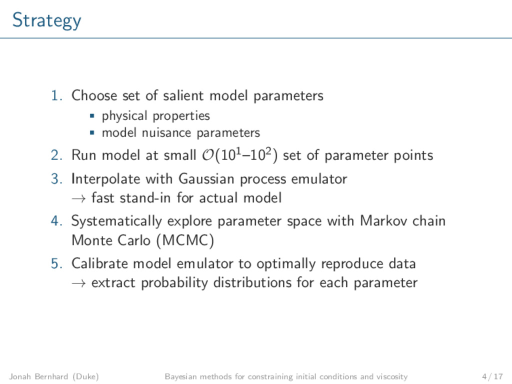
5. Strategy 1. Choose set of salient model parameters physical properties model nuisance parameters 2. Run model at small O(101–102) set of parameter points 3. Interpolate with Gaussian process emulator → fast stand-in for actual model 4. Systematically explore parameter space with Markov chain Monte Carlo (MCMC) 5. Calibrate model emulator to optimally reproduce data → extract probability distributions for each parameter Jonah Bernhard (Duke) Bayesian methods for constraining initial conditions and viscosity 4 / 17
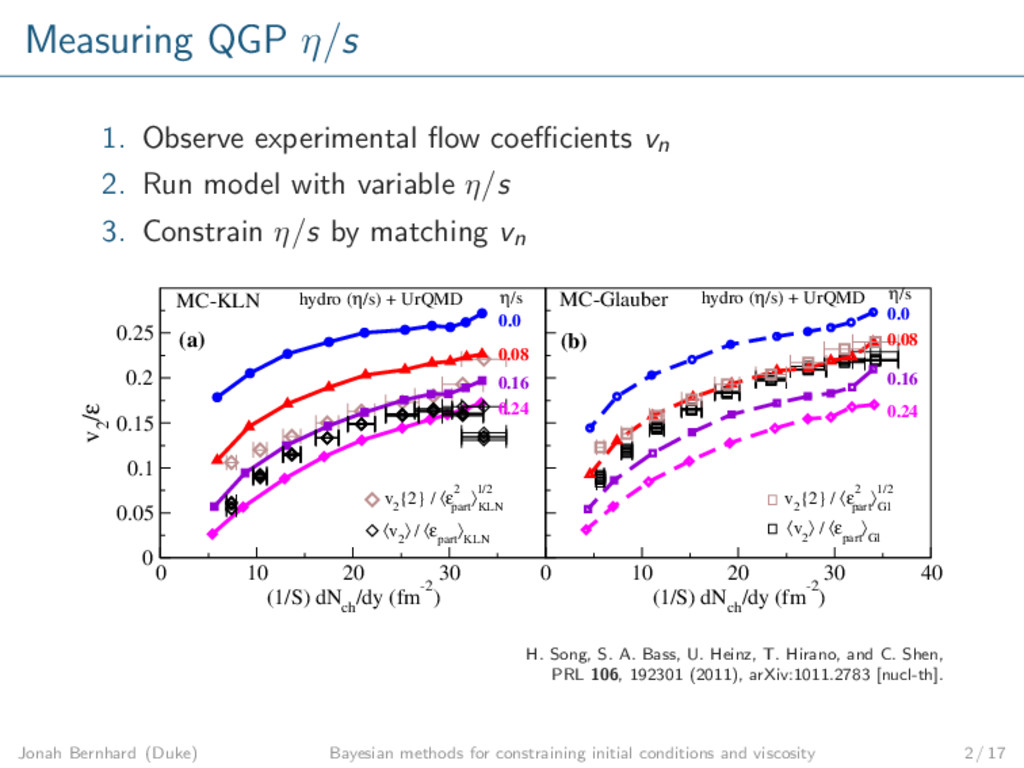
6. Event-by-event model MC-Glauber & MC-KLN initial conditions H.-J. Drescher and Y. Nara, PRC 74, 044905 (2006). Viscous 2+1D hydro H. Song and U. Heinz, PRC 77, 064901 (2008). Cooper-Frye hypersurface sampler C. Shen, Z. Qiu, H. Song, J. Bernhard, S. Bass, and U. Heinz, arXiv:1409.8164 [nucl-th]. UrQMD S. Bass et. al., Prog. Part. Nucl. Phys. 41, 255 (1998). M. Bleicher et. al., J. Phys. G 25, 1859 (1999). Jonah Bernhard (Duke) Bayesian methods for constraining initial conditions and viscosity 5 / 17
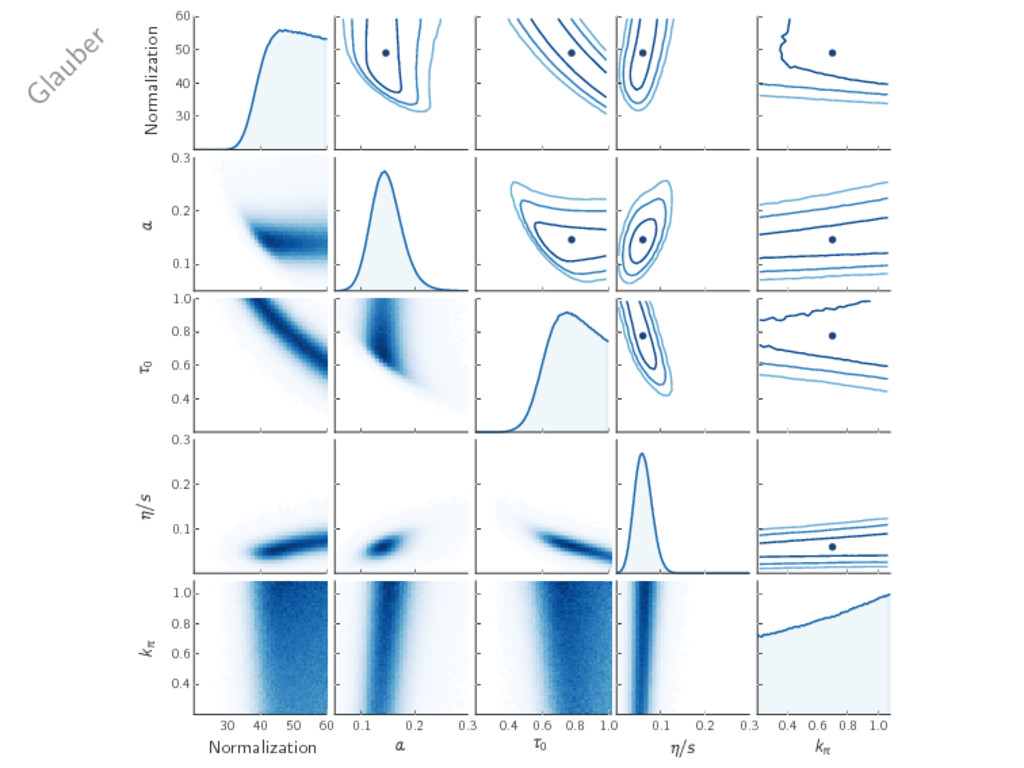
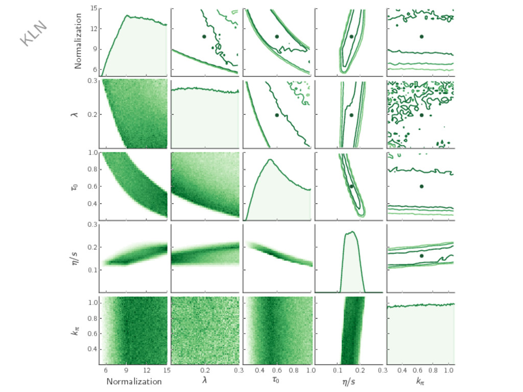
7. Calibration parameters Initial condition parameters: Overall normalization factor α (Glauber), λ (KLN) → both control centrality dependence of multiplicity Hydro parameters: Thermalization time τ0 Specific shear viscosity η/s Shear relaxation time τπ = 6kπη/(sT) [vary kπ] Design: 250 points in parameter space O(104) events at each point All parameters varied simultaneously Jonah Bernhard (Duke) Bayesian methods for constraining initial conditions and viscosity 6 / 17
8. Training data Model calculations at each parameter point 0 2000 4000 6000 Glauber ­ Nch ® 0.00 0.04 0.08 0.12 v2 {2} 0.00 0.02 0.04 v3 {2} 0 10 20 30 40 50 Centrality % 0 2000 4000 6000 KLN 0 10 20 30 40 50 Centrality % 0.00 0.04 0.08 0.12 0 10 20 30 40 50 Centrality % 0.00 0.02 0.04 Data points: ALICE Collaboration, Pb-Pb collisions at √ sNN = 2.76 TeV B. B. Abelev et al., PRC 90, 054901 (2014), arXiv:1406.2474 [nucl-ex]. Jonah Bernhard (Duke) Bayesian methods for constraining initial conditions and viscosity 7 / 17
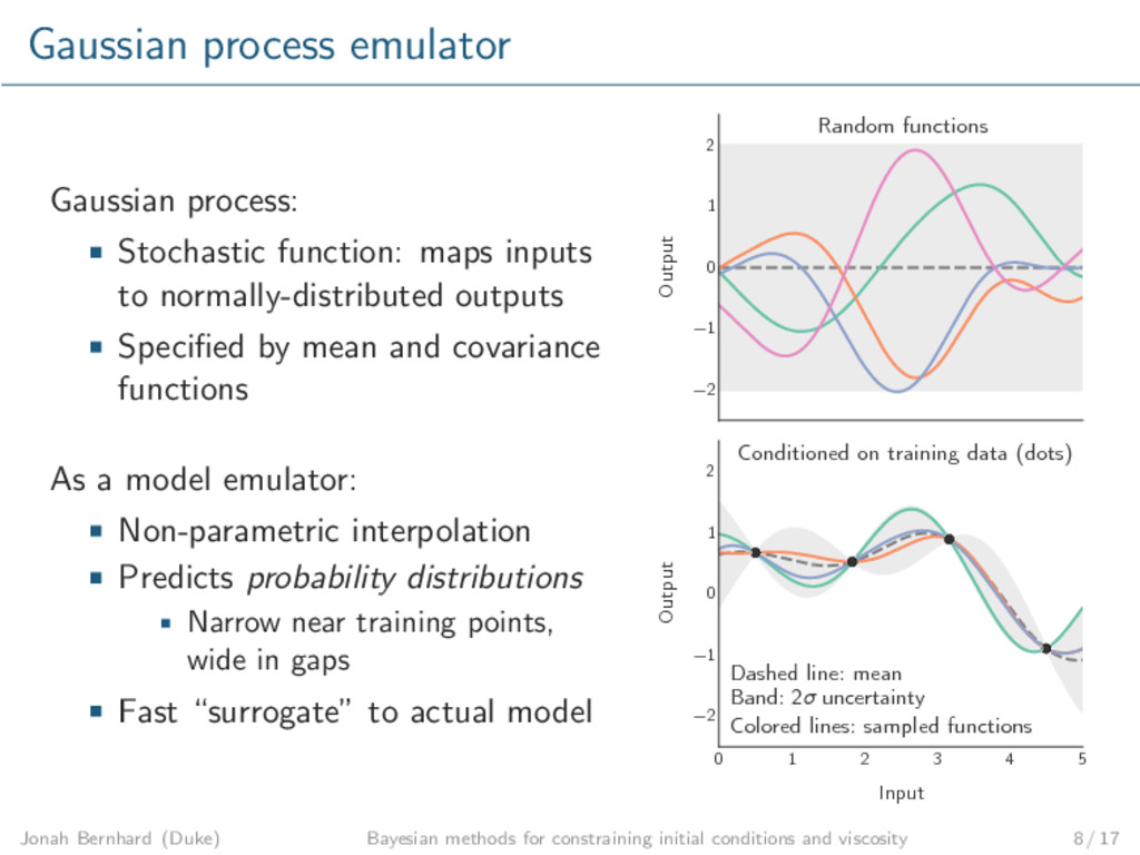
9. Gaussian process emulator Gaussian process: Stochastic function: maps inputs to normally-distributed outputs Specified by mean and covariance functions As a model emulator: Non-parametric interpolation Predicts probability distributions Narrow near training points, wide in gaps Fast “surrogate” to actual model −2 −1 0 1 2 Output Random functions 0 1 2 3 4 5 Input −2 −1 0 1 2 Output Dashed line: mean Band: 2σ uncertainty Colored lines: sampled functions Conditioned on training data (dots) Jonah Bernhard (Duke) Bayesian methods for constraining initial conditions and viscosity 8 / 17
10. Validation Independent set of validation points Run model and predict output with emulator at each point Accurate predictions fall on diagonal line 0 2500 5000 Predicted ­ Nch ® 2500 5000 Observed 0–5% 20–25% 40–45% 0.00 0.04 0.08 0.12 Predicted v2 {2} 0.04 0.08 0.12 0.00 0.02 0.04 Predicted v3 {2} 0.02 0.04 Horizontal error bars: 2σ emulator uncertainty Vertical error bars: 2σ statistical uncertainty Jonah Bernhard (Duke) Bayesian methods for constraining initial conditions and viscosity 9 / 17
11. Calibration Input parameters: x = (Norm, I.C. param, τ0, η/s, kπ) → find posterior probability distribution of true parameters x Markov chain Monte Carlo (MCMC): Directly samples probability P(x ) ∼ exp − (x − xexp)2 2σ2 Random walk through parameter space Large number of samples → chain equilibrates to posterior distribution Jonah Bernhard (Duke) Bayesian methods for constraining initial conditions and viscosity 10 / 17
12. Posterior distributions
13. 30 40 50 60 Normalization 0.1 0.2 0.3 α 0.4 0.6 0.8 1.0 τ0 0.1 0.2 0.3 η/s 30 40 50 60 Normalization 0.4 0.6 0.8 1.0 kπ 0.1 0.2 0.3 α 0.4 0.6 0.8 1.0 τ0 0.1 0.2 0.3 η/s 0.4 0.6 0.8 1.0 kπ Glauber
14. 6 9 12 15 Normalization 0.2 0.3 λ 0.4 0.6 0.8 1.0 τ0 0.1 0.2 0.3 η/s 6 9 12 15 Normalization 0.4 0.6 0.8 1.0 kπ 0.2 0.3 λ 0.4 0.6 0.8 1.0 τ0 0.1 0.2 0.3 η/s 0.4 0.6 0.8 1.0 kπ KLN
15. Posterior samples Model calculations over full design space 0 2000 4000 6000 Glauber ­ Nch ® 0.00 0.04 0.08 0.12 v2 {2} 0.00 0.02 0.04 v3 {2} 0 10 20 30 40 50 Centrality % 0 2000 4000 6000 KLN 0 10 20 30 40 50 Centrality % 0.00 0.04 0.08 0.12 0 10 20 30 40 50 Centrality % 0.00 0.02 0.04 Jonah Bernhard (Duke) Bayesian methods for constraining initial conditions and viscosity 13 / 17
16. Posterior samples Emulator predictions from calibrated posterior 0 2000 4000 6000 Glauber ­ Nch ® 0.00 0.04 0.08 0.12 v2 {2} 0.00 0.02 0.04 v3 {2} 0 10 20 30 40 50 Centrality % 0 2000 4000 6000 KLN 0 10 20 30 40 50 Centrality % 0.00 0.04 0.08 0.12 0 10 20 30 40 50 Centrality % 0.00 0.02 0.04 Jonah Bernhard (Duke) Bayesian methods for constraining initial conditions and viscosity 13 / 17
17. η/s posteriors Glauber η/s ∼ 0.06, 95% C.I. ∼ 0.02–0.10 KLN η/s ∼ 0.16, 95% C.I. ∼ 0.12–0.21 0.0 0.1 0.2 0.3 η/s Glauber 0.08 KLN 0.20 Jonah Bernhard (Duke) Bayesian methods for constraining initial conditions and viscosity 14 / 17
18. Sensitivity Go to posterior mean Vary one parameter at a time; keep others fixed at mean Emulate response of each observable
19. 0 1000 2000 3000 4000 ­ Nch ® 0.00 0.03 0.06 0.09 0.12 v2 {2} 20 30 40 50 60 Normalization 0.00 0.01 0.02 0.03 v3 {2} 0–5% 20–25% 40–45% 0.1 0.2 0.3 α x = posterior mean band = 1σ C.I. 0.2 0.4 0.6 0.8 1.0 τ0 y = ALICE value band = uncertainty 0.0 0.1 0.2 0.3 η/s 0.2 0.4 0.6 0.8 1.0 kπ Glauber
20. 0 1000 2000 3000 4000 ­ Nch ® 0.00 0.03 0.06 0.09 0.12 v2 {2} 6 9 12 15 Normalization 0.00 0.01 0.02 0.03 v3 {2} 0–5% 20–25% 40–45% 0.1 0.2 0.3 λ x = posterior mean band = 1σ C.I. 0.2 0.4 0.6 0.8 1.0 τ0 y = ALICE value band = uncertainty 0.0 0.1 0.2 0.3 η/s 0.2 0.4 0.6 0.8 1.0 kπ KLN
21. Summary Quantitative, systematic parameter extraction and model evaluation Glauber approximately describes Nch, v2, v3 KLN cannot simultaneously fit v2, v3 Next: Initial condition models Trento (J. S. Moreland, J. E. Bernhard, S. A. Bass, arXiv:1412.4708 [nucl-th].) fluctuated Glauber More input parameters: nucleon size, Tswitch More observables: pT , v2{4}, HBT, identified particles RHIC and LHC Improve treatment of uncertainty Jonah Bernhard (Duke) Bayesian methods for constraining initial conditions and viscosity 17 / 17
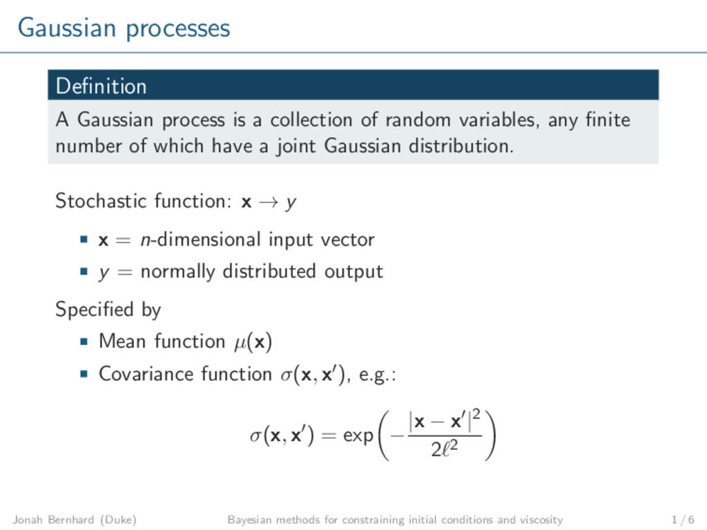
22. Gaussian processes Definition A Gaussian process is a collection of random variables, any finite number of which have a joint Gaussian distribution. Stochastic function: x → y x = n-dimensional input vector y = normally distributed output Specified by Mean function µ(x) Covariance function σ(x, x ), e.g.: σ(x, x ) = exp − |x − x |2 2 2 Jonah Bernhard (Duke) Bayesian methods for constraining initial conditions and viscosity 1 / 6
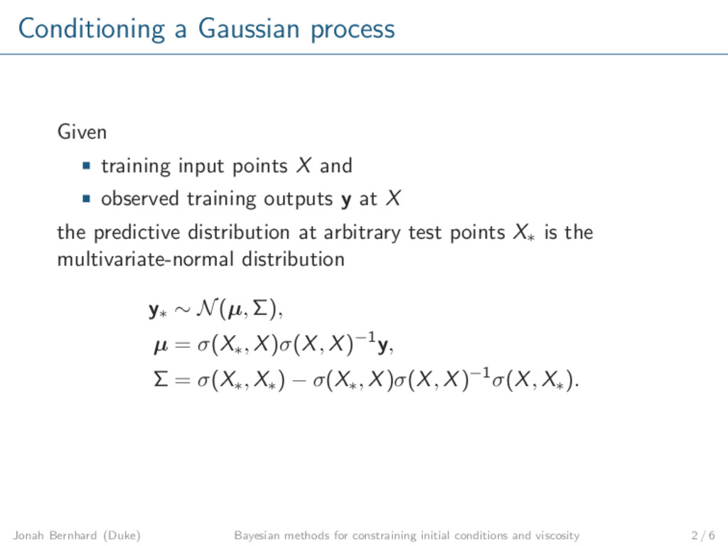
23. Conditioning a Gaussian process Given training input points X and observed training outputs y at X the predictive distribution at arbitrary test points X∗ is the multivariate-normal distribution y∗ ∼ N(µ, Σ), µ = σ(X∗, X)σ(X, X)−1y, Σ = σ(X∗, X∗) − σ(X∗, X)σ(X, X)−1σ(X, X∗). Jonah Bernhard (Duke) Bayesian methods for constraining initial conditions and viscosity 2 / 6
24. Training the emulator Covariance function: σ(x, x ) = exp − |x − x |2 2 2 + σ2 n δxx ( , σn) are unknown hyperparameters 0.0 0.2 0.4 0.6 0.8 1.0 x −2 −1 0 1 2 y Overfit ` = 0.02, σn = 0.001 0.0 0.2 0.4 0.6 0.8 1.0 x Oversmooth ` = 3, σn = 0.3 0.0 0.2 0.4 0.6 0.8 1.0 x Max. likelihood ` = 0.462, σn = 0.211 Actual ` = 0.5, σn = 0.2 Jonah Bernhard (Duke) Bayesian methods for constraining initial conditions and viscosity 3 / 6
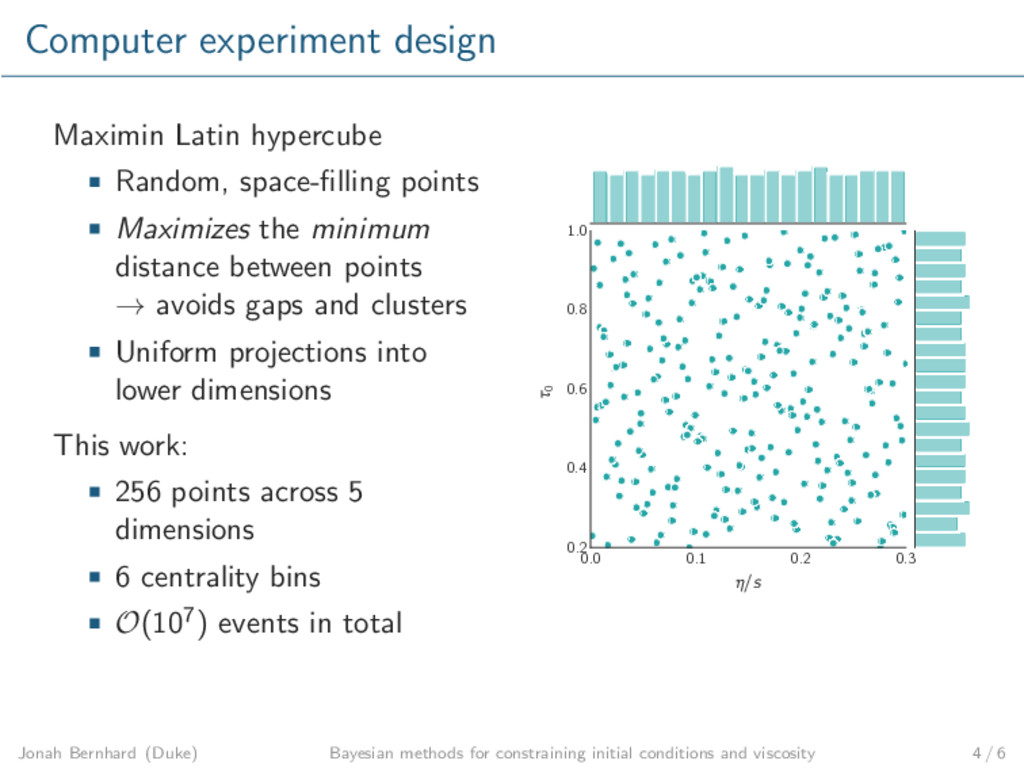
25. Computer experiment design Maximin Latin hypercube Random, space-filling points Maximizes the minimum distance between points → avoids gaps and clusters Uniform projections into lower dimensions This work: 256 points across 5 dimensions 6 centrality bins O(107) events in total 0.0 0.1 0.2 0.3 η/s 0.2 0.4 0.6 0.8 1.0 τ0 Jonah Bernhard (Duke) Bayesian methods for constraining initial conditions and viscosity 4 / 6
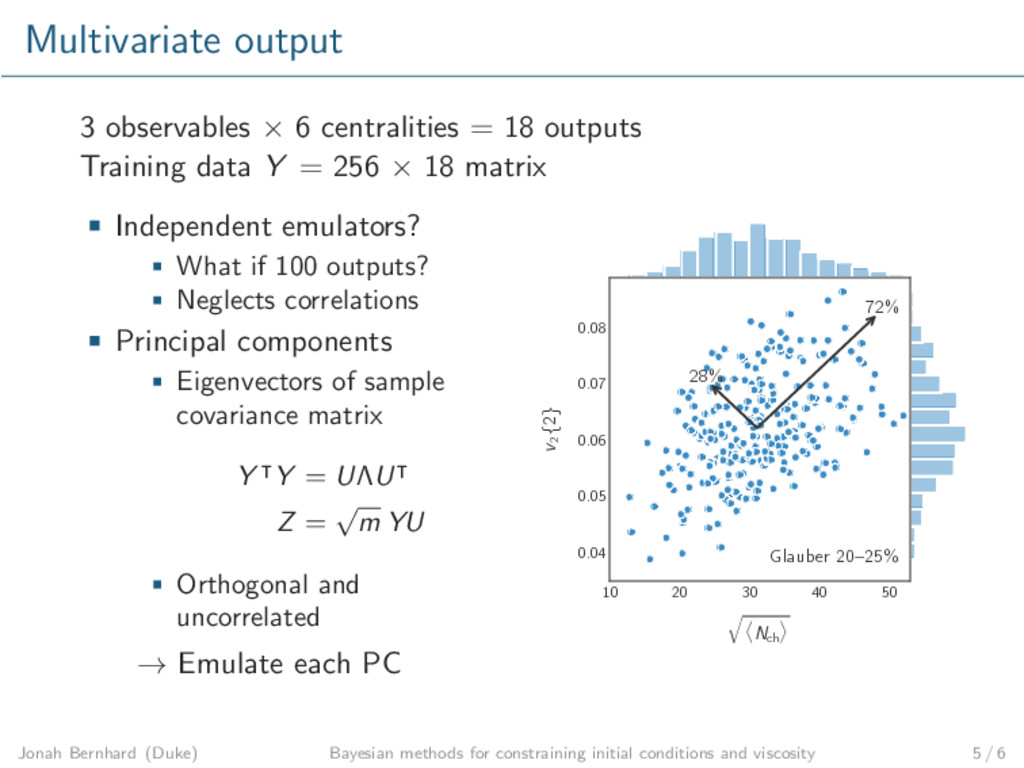
26. Multivariate output 3 observables × 6 centralities = 18 outputs Training data Y = 256 × 18 matrix Independent emulators? What if 100 outputs? Neglects correlations Principal components Eigenvectors of sample covariance matrix Y Y = UΛU Z = √ m YU Orthogonal and uncorrelated → Emulate each PC 10 20 30 40 50 q­ Nch ® 0.04 0.05 0.06 0.07 0.08 v2 {2} Glauber 20–25% 72% 28% Jonah Bernhard (Duke) Bayesian methods for constraining initial conditions and viscosity 5 / 6
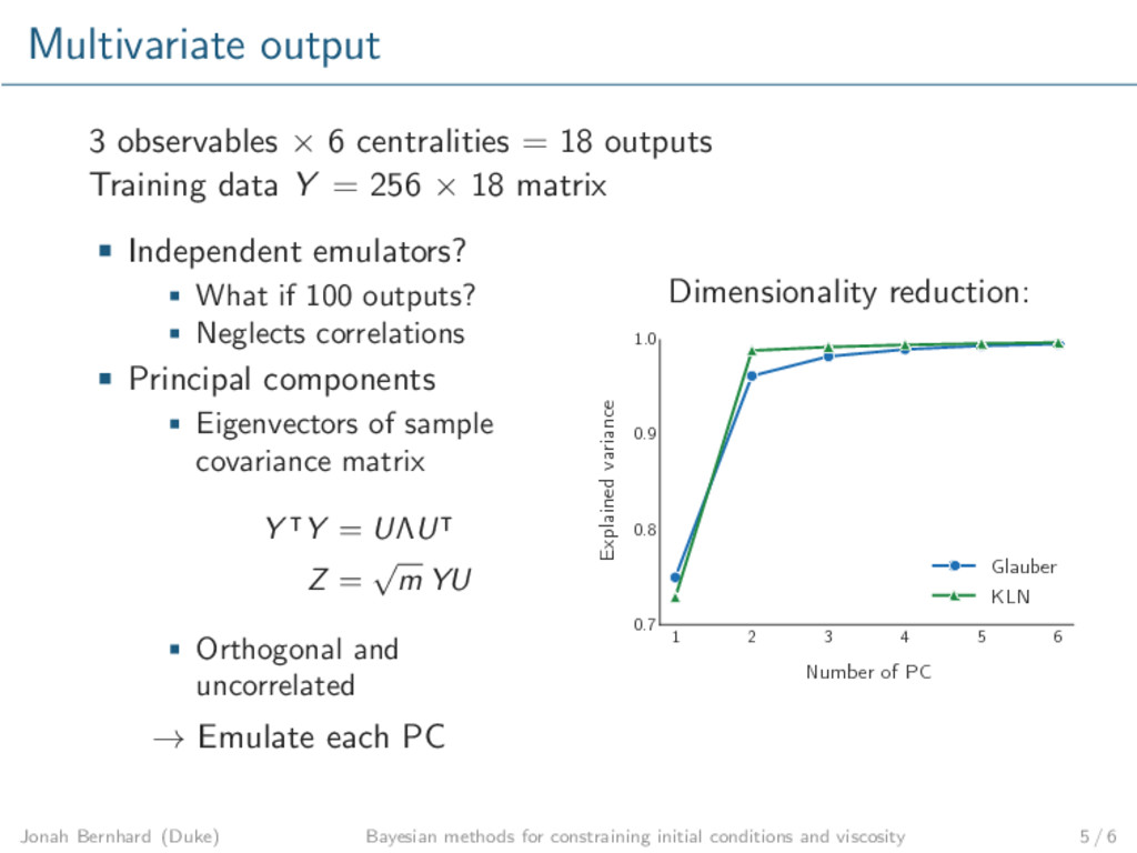
27. Multivariate output 3 observables × 6 centralities = 18 outputs Training data Y = 256 × 18 matrix Independent emulators? What if 100 outputs? Neglects correlations Principal components Eigenvectors of sample covariance matrix Y Y = UΛU Z = √ m YU Orthogonal and uncorrelated → Emulate each PC Dimensionality reduction: 1 2 3 4 5 6 Number of PC 0.7 0.8 0.9 1.0 Explained variance Glauber KLN Jonah Bernhard (Duke) Bayesian methods for constraining initial conditions and viscosity 5 / 6
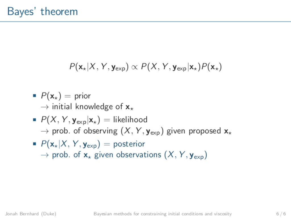
28. Bayes’ theorem P(x |X, Y , yexp) ∝ P(X, Y , yexp|x )P(x ) P(x ) = prior → initial knowledge of x P(X, Y , yexp|x ) = likelihood → prob. of observing (X, Y , yexp) given proposed x P(x |X, Y , yexp) = posterior → prob. of x given observations (X, Y , yexp) Jonah Bernhard (Duke) Bayesian methods for constraining initial conditions and viscosity 6 / 6