Quantifying properties of hot and dense QCD matter through systematic model-to-data comparison

Presented at the Institute for Nuclear Theory, University of Washington http://www.int.washington.edu/PROGRAMS/15-2b

Transcript

1. Quantifying properties of hot and dense QCD matter through systematic model-to-data comparison Jonah Bernhard INT workshop: Correlations and fluctuations in p+A and A+A collisions Tuesday, July 14, 2015 J. E. Bernhard, P. W. Marcy, C. E. Coleman-Smith, S. Huzurbazar, R. L. Wolpert, and S. A. Bass, PRC 91, 054910 (2015), arXiv:1502.00339 [nucl-th].
2. Model-to-data comparison | < 1) lab η (| ch N 50 100 150 200 c < 3.0 GeV/ T p < | > 1.4} η ∆ {2, | 2 v {4} 2 v = 5.02 TeV NN s ICE p-Pb | < 1) lab η (| ch N 10 2 10 3 10 2 v 0 0.02 0.04 0.06 0.08 0.1 0.12 | > 1.4} η ∆ {2, | 2 v {4} 2 v {6} 2 v 82 65 52 43 31 17 7 Centrality (%) c < 3.0 GeV/ T p 0.2 < = 2.76 TeV NN s ALICE Pb-Pb Model Initial conditions, τ0, η/s, . . . 0 2000 4000 6000 Glauber ­ Nch ® 0.00 0.04 0.08 0.12 v2 {2} 0.00 0.02 0.04 v3 {2} 0 10 20 30 40 50 Centrality % 0 2000 4000 6000 KLN 0 10 20 30 40 50 Centrality % 0.00 0.04 0.08 0.12 0 10 20 30 40 50 Centrality % 0.00 0.02 0.04 Jonah Bernhard (Duke) Quantifying QGP properties through model-to-data comparison 1 / 22
3. Measuring QGP η/s 1. Observe experimental flow coefficients vn 2. Run model with variable η/s 3. Constrain η/s by matching vn 0 10 20 30 (1/S) dN ch /dy (fm-2 ) 0 0.05 0.1 0.15 0.2 0.25 v 2 /ε 0 10 20 30 40 (1/S) dN ch /dy (fm-2 ) hydro (η/s) + UrQMD hydro (η/s) + UrQMD MC-Glauber MC-KLN 0.0 0.08 0.16 0.24 0.0 0.08 0.16 0.24 η/s η/s v 2 {2} / 〈ε2 part 〉1/2 Gl (a) (b) 〈v 2 〉 / 〈ε part 〉 Gl v 2 {2} / 〈ε2 part 〉1/2 KLN 〈v 2 〉 / 〈ε part 〉 KLN H. Song, S. A. Bass, U. Heinz, T. Hirano, and C. Shen, PRL 106, 192301 (2011), arXiv:1011.2783 [nucl-th]. Jonah Bernhard (Duke) Quantifying QGP properties through model-to-data comparison 2 / 22
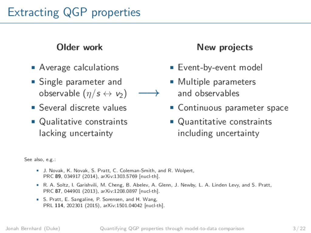
4. Extracting QGP properties Older work Average calculations Single parameter and observable (η/s ↔ v2) Several discrete values Qualitative constraints lacking uncertainty New projects Event-by-event model Multiple parameters and observables Continuous parameter space Quantitative constraints including uncertainty See also, e.g.: J. Novak, K. Novak, S. Pratt, C. Coleman-Smith, and R. Wolpert, PRC 89, 034917 (2014), arXiv:1303.5769 [nucl-th]. R. A. Soltz, I. Garishvili, M. Cheng, B. Abelev, A. Glenn, J. Newby, L. A. Linden Levy, and S. Pratt, PRC 87, 044901 (2013), arXiv:1208.0897 [nucl-th]. S. Pratt, E. Sangaline, P. Sorensen, and H. Wang, PRL 114, 202301 (2015), arXiv:1501.04042 [nucl-th]. −→ Jonah Bernhard (Duke) Quantifying QGP properties through model-to-data comparison 3 / 22
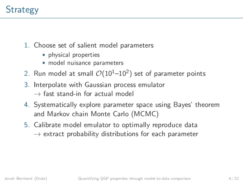
5. Strategy 1. Choose set of salient model parameters physical properties model nuisance parameters 2. Run model at small O(101–102) set of parameter points 3. Interpolate with Gaussian process emulator → fast stand-in for actual model 4. Systematically explore parameter space using Bayes’ theorem and Markov chain Monte Carlo (MCMC) 5. Calibrate model emulator to optimally reproduce data → extract probability distributions for each parameter Jonah Bernhard (Duke) Quantifying QGP properties through model-to-data comparison 4 / 22
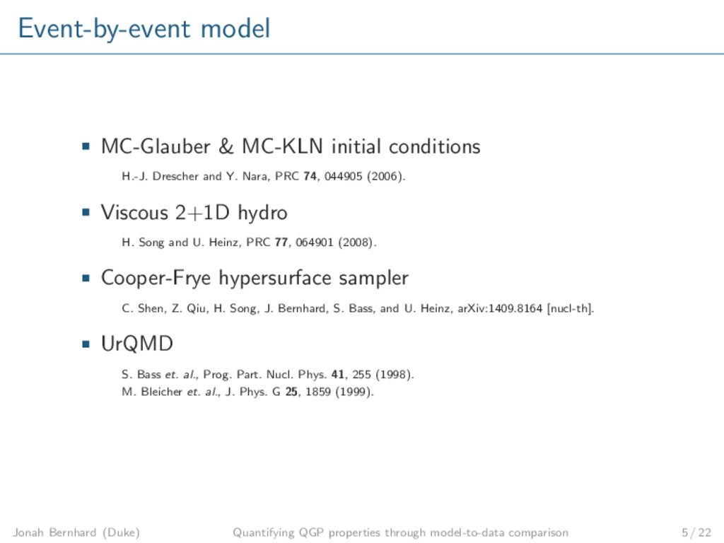
6. Event-by-event model MC-Glauber & MC-KLN initial conditions H.-J. Drescher and Y. Nara, PRC 74, 044905 (2006). Viscous 2+1D hydro H. Song and U. Heinz, PRC 77, 064901 (2008). Cooper-Frye hypersurface sampler C. Shen, Z. Qiu, H. Song, J. Bernhard, S. Bass, and U. Heinz, arXiv:1409.8164 [nucl-th]. UrQMD S. Bass et. al., Prog. Part. Nucl. Phys. 41, 255 (1998). M. Bleicher et. al., J. Phys. G 25, 1859 (1999). Jonah Bernhard (Duke) Quantifying QGP properties through model-to-data comparison 5 / 22
7. Calibration parameters Initial condition parameters: Overall normalization factor α (Glauber), λ (KLN) → both control centrality dependence of multiplicity Hydro parameters: Thermalization time τ0 Specific shear viscosity η/s Shear relaxation time τπ = 6kπη/(sT) [vary kπ] Jonah Bernhard (Duke) Quantifying QGP properties through model-to-data comparison 6 / 22
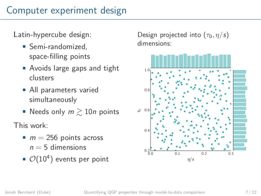
8. Computer experiment design Latin-hypercube design: Semi-randomized, space-filling points Avoids large gaps and tight clusters All parameters varied simultaneously Needs only m 10n points This work: m = 256 points across n = 5 dimensions O(104) events per point Design projected into (τ0, η/s) dimensions: 0.0 0.1 0.2 0.3 η/s 0.2 0.4 0.6 0.8 1.0 τ0 Jonah Bernhard (Duke) Quantifying QGP properties through model-to-data comparison 7 / 22
9. Training data Model calculations at each parameter point 0 2000 4000 6000 Glauber ­ Nch ® 0.00 0.04 0.08 0.12 v2 {2} 0.00 0.02 0.04 v3 {2} 0 10 20 30 40 50 Centrality % 0 2000 4000 6000 KLN 0 10 20 30 40 50 Centrality % 0.00 0.04 0.08 0.12 0 10 20 30 40 50 Centrality % 0.00 0.02 0.04 Data points: ALICE Collaboration, Pb-Pb collisions at √ sNN = 2.76 TeV B. B. Abelev et al., PRC 90, 054901 (2014), arXiv:1406.2474 [nucl-ex]. Jonah Bernhard (Duke) Quantifying QGP properties through model-to-data comparison 8 / 22
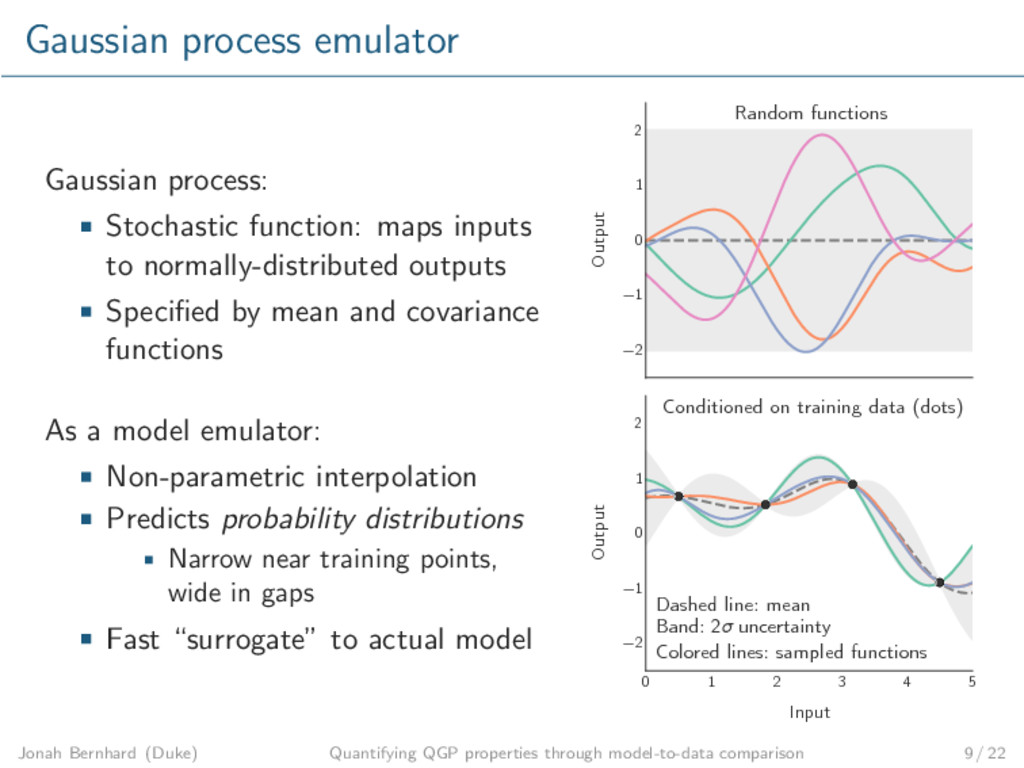
10. Gaussian process emulator Gaussian process: Stochastic function: maps inputs to normally-distributed outputs Specified by mean and covariance functions As a model emulator: Non-parametric interpolation Predicts probability distributions Narrow near training points, wide in gaps Fast “surrogate” to actual model −2 −1 0 1 2 Output Random functions 0 1 2 3 4 5 Input −2 −1 0 1 2 Output Dashed line: mean Band: 2σ uncertainty Colored lines: sampled functions Conditioned on training data (dots) Jonah Bernhard (Duke) Quantifying QGP properties through model-to-data comparison 9 / 22
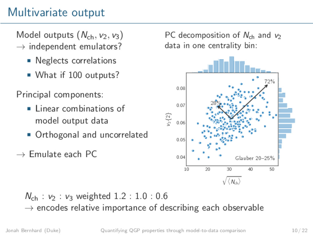
11. Multivariate output Model outputs (Nch, v2, v3) → independent emulators? Neglects correlations What if 100 outputs? Principal components: Linear combinations of model output data Orthogonal and uncorrelated → Emulate each PC PC decomposition of Nch and v2 data in one centrality bin: 10 20 30 40 50 q­ Nch ® 0.04 0.05 0.06 0.07 0.08 v2 {2} Glauber 20–25% 72% 28% Nch : v2 : v3 weighted 1.2 : 1.0 : 0.6 → encodes relative importance of describing each observable Jonah Bernhard (Duke) Quantifying QGP properties through model-to-data comparison 10 / 22
12. Validation Independent set of validation points Run model and predict output with emulator at each point Accurate predictions fall on diagonal line 0 2500 5000 Predicted ­ Nch ® 2500 5000 Observed 0–5% 20–25% 40–45% 0.00 0.04 0.08 0.12 Predicted v2 {2} 0.04 0.08 0.12 0.00 0.02 0.04 Predicted v3 {2} 0.02 0.04 Horizontal error bars: 2σ emulator uncertainty Vertical error bars: 2σ statistical uncertainty Jonah Bernhard (Duke) Quantifying QGP properties through model-to-data comparison 11 / 22
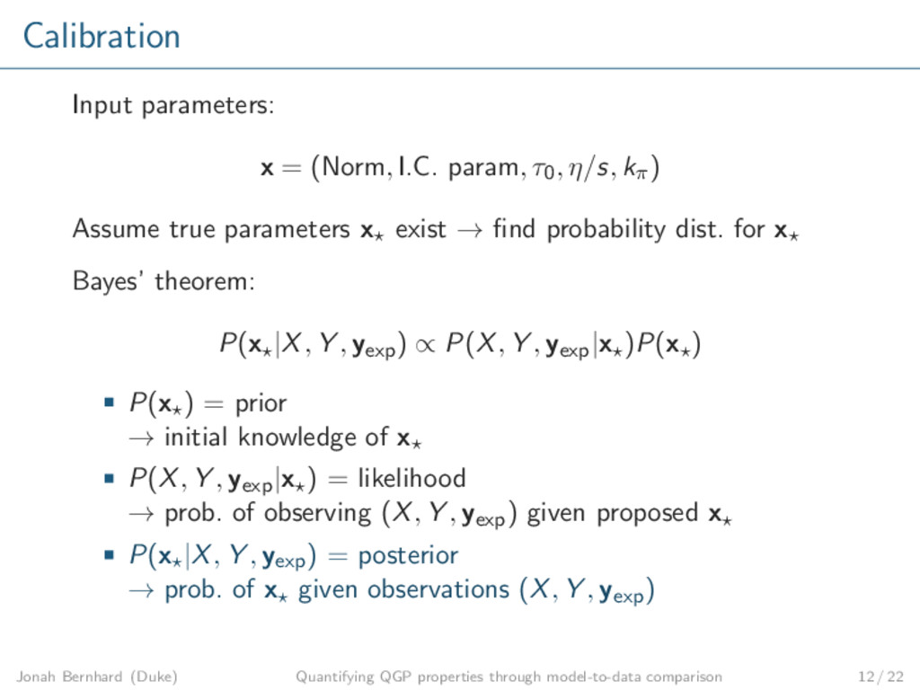
13. Calibration Input parameters: x = (Norm, I.C. param, τ0, η/s, kπ) Assume true parameters x exist → find probability dist. for x Bayes’ theorem: P(x |X, Y , yexp) ∝ P(X, Y , yexp|x )P(x ) P(x ) = prior → initial knowledge of x P(X, Y , yexp|x ) = likelihood → prob. of observing (X, Y , yexp) given proposed x P(x |X, Y , yexp) = posterior → prob. of x given observations (X, Y , yexp) Jonah Bernhard (Duke) Quantifying QGP properties through model-to-data comparison 12 / 22
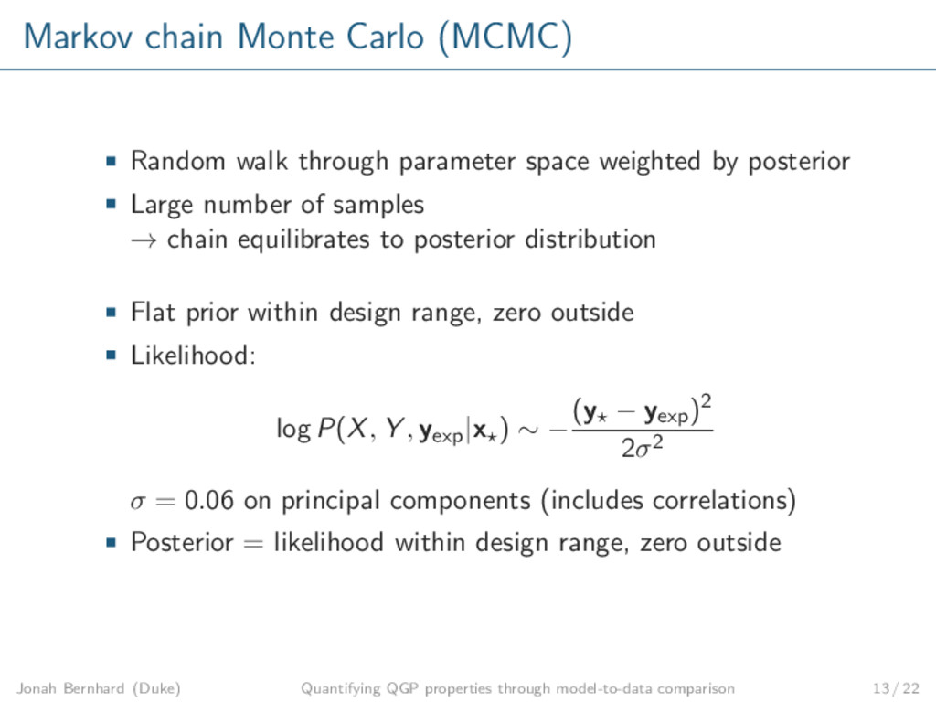
14. Markov chain Monte Carlo (MCMC) Random walk through parameter space weighted by posterior Large number of samples → chain equilibrates to posterior distribution Flat prior within design range, zero outside Likelihood: log P(X, Y , yexp|x ) ∼ − (y − yexp)2 2σ2 σ = 0.06 on principal components (includes correlations) Posterior = likelihood within design range, zero outside Jonah Bernhard (Duke) Quantifying QGP properties through model-to-data comparison 13 / 22
15. η/s posteriors Glauber η/s ∼ 0.06, 95% C.I. ∼ 0.02–0.10 KLN η/s ∼ 0.16, 95% C.I. ∼ 0.12–0.21 0.0 0.1 0.2 0.3 η/s Glauber 0.08 KLN 0.20 Jonah Bernhard (Duke) Quantifying QGP properties through model-to-data comparison 14 / 22
16. 30 40 50 60 Normalization 0.1 0.2 0.3 α 0.4 0.6 0.8 1.0 τ0 0.1 0.2 0.3 η/s 30 40 50 60 Normalization 0.4 0.6 0.8 1.0 kπ 0.1 0.2 0.3 α 0.4 0.6 0.8 1.0 τ0 0.1 0.2 0.3 η/s 0.4 0.6 0.8 1.0 kπ Glauber
17. 6 9 12 15 Normalization 0.2 0.3 λ 0.4 0.6 0.8 1.0 τ0 0.1 0.2 0.3 η/s 6 9 12 15 Normalization 0.4 0.6 0.8 1.0 kπ 0.2 0.3 λ 0.4 0.6 0.8 1.0 τ0 0.1 0.2 0.3 η/s 0.4 0.6 0.8 1.0 kπ KLN
18. Posterior samples Model calculations over full design space 0 2000 4000 6000 Glauber ­ Nch ® 0.00 0.04 0.08 0.12 v2 {2} 0.00 0.02 0.04 v3 {2} 0 10 20 30 40 50 Centrality % 0 2000 4000 6000 KLN 0 10 20 30 40 50 Centrality % 0.00 0.04 0.08 0.12 0 10 20 30 40 50 Centrality % 0.00 0.02 0.04 Jonah Bernhard (Duke) Quantifying QGP properties through model-to-data comparison 17 / 22
19. Posterior samples Emulator predictions from calibrated posterior 0 2000 4000 6000 Glauber ­ Nch ® 0.00 0.04 0.08 0.12 v2 {2} 0.00 0.02 0.04 v3 {2} 0 10 20 30 40 50 Centrality % 0 2000 4000 6000 KLN 0 10 20 30 40 50 Centrality % 0.00 0.04 0.08 0.12 0 10 20 30 40 50 Centrality % 0.00 0.02 0.04 Jonah Bernhard (Duke) Quantifying QGP properties through model-to-data comparison 17 / 22
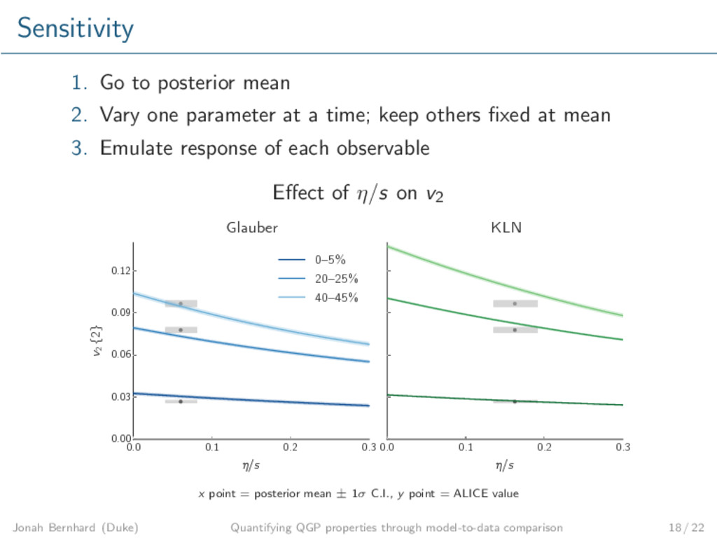
20. Sensitivity 1. Go to posterior mean 2. Vary one parameter at a time; keep others fixed at mean 3. Emulate response of each observable Effect of η/s on v2 0.0 0.1 0.2 0.3 η/s 0.00 0.03 0.06 0.09 0.12 v2 {2} Glauber 0–5% 20–25% 40–45% 0.0 0.1 0.2 0.3 η/s KLN x point = posterior mean ± 1σ C.I., y point = ALICE value Jonah Bernhard (Duke) Quantifying QGP properties through model-to-data comparison 18 / 22
21. 0 1000 2000 3000 4000 ­ Nch ® 0.00 0.03 0.06 0.09 0.12 v2 {2} 20 30 40 50 60 Normalization 0.00 0.01 0.02 0.03 v3 {2} 0–5% 20–25% 40–45% 0.1 0.2 0.3 α x = posterior mean band = 1σ C.I. 0.2 0.4 0.6 0.8 1.0 τ0 y = ALICE value band = uncertainty 0.0 0.1 0.2 0.3 η/s 0.2 0.4 0.6 0.8 1.0 kπ Glauber
22. 0 1000 2000 3000 4000 ­ Nch ® 0.00 0.03 0.06 0.09 0.12 v2 {2} 6 9 12 15 Normalization 0.00 0.01 0.02 0.03 v3 {2} 0–5% 20–25% 40–45% 0.1 0.2 0.3 λ x = posterior mean band = 1σ C.I. 0.2 0.4 0.6 0.8 1.0 τ0 y = ALICE value band = uncertainty 0.0 0.1 0.2 0.3 η/s 0.2 0.4 0.6 0.8 1.0 kπ KLN
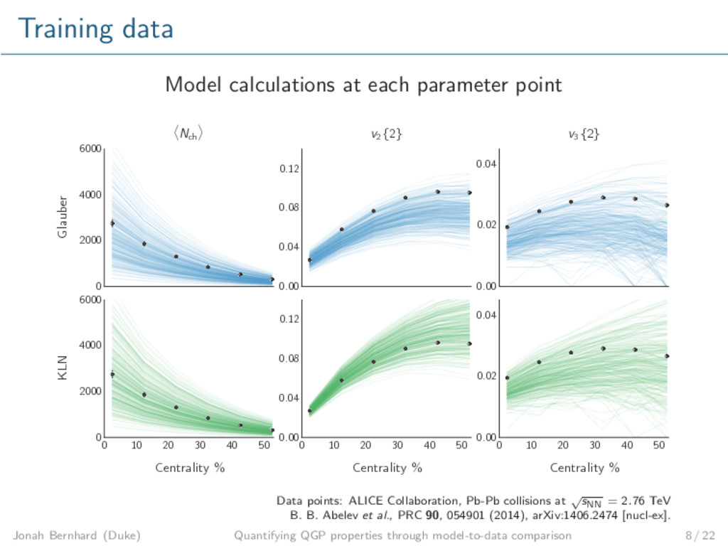
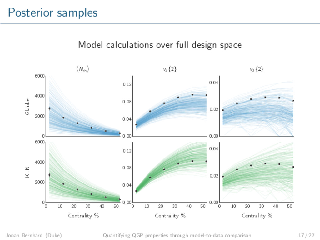
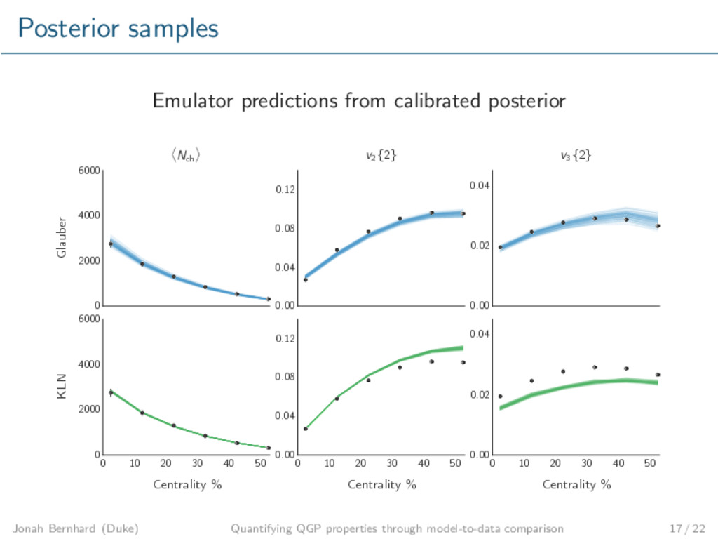
23. Summary Framework for quantitative, systematic parameter extraction and model evaluation Gaussian process emulator accurately predicts model output MCMC gives full probability distributions for all parameters Glauber approximately describes Nch, v2, v3 KLN cannot simultaneously fit v2, v3 Jonah Bernhard (Duke) Quantifying QGP properties through model-to-data comparison 21 / 22
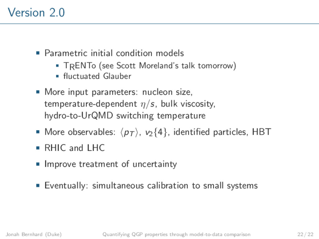
24. Version 2.0 Parametric initial condition models TRENTo (see Scott Moreland’s talk tomorrow) fluctuated Glauber More input parameters: nucleon size, temperature-dependent η/s, bulk viscosity, hydro-to-UrQMD switching temperature More observables: pT , v2{4}, identified particles, HBT RHIC and LHC Improve treatment of uncertainty Eventually: simultaneous calibration to small systems Jonah Bernhard (Duke) Quantifying QGP properties through model-to-data comparison 22 / 22
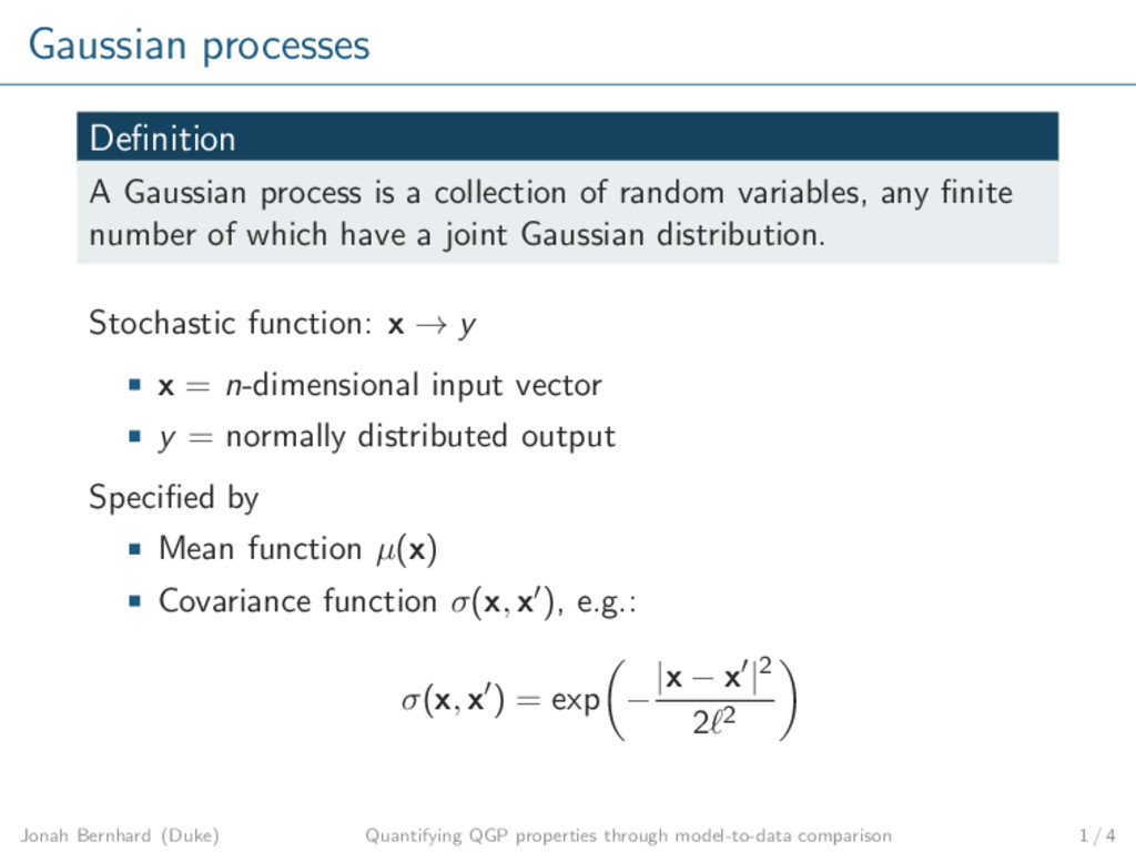
25. Gaussian processes Definition A Gaussian process is a collection of random variables, any finite number of which have a joint Gaussian distribution. Stochastic function: x → y x = n-dimensional input vector y = normally distributed output Specified by Mean function µ(x) Covariance function σ(x, x ), e.g.: σ(x, x ) = exp − |x − x |2 2 2 Jonah Bernhard (Duke) Quantifying QGP properties through model-to-data comparison 1 / 4
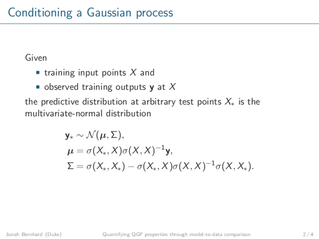
26. Conditioning a Gaussian process Given training input points X and observed training outputs y at X the predictive distribution at arbitrary test points X∗ is the multivariate-normal distribution y∗ ∼ N(µ, Σ), µ = σ(X∗, X)σ(X, X)−1y, Σ = σ(X∗, X∗) − σ(X∗, X)σ(X, X)−1σ(X, X∗). Jonah Bernhard (Duke) Quantifying QGP properties through model-to-data comparison 2 / 4
27. Training the emulator Covariance function: σ(x, x ) = exp − |x − x |2 2 2 + σ2 n δxx ( , σn) are unknown hyperparameters 0.0 0.2 0.4 0.6 0.8 1.0 x −2 −1 0 1 2 y Overfit ` = 0.02, σn = 0.001 0.0 0.2 0.4 0.6 0.8 1.0 x Oversmooth ` = 3, σn = 0.3 0.0 0.2 0.4 0.6 0.8 1.0 x Max. likelihood ` = 0.462, σn = 0.211 Actual ` = 0.5, σn = 0.2 Jonah Bernhard (Duke) Quantifying QGP properties through model-to-data comparison 3 / 4
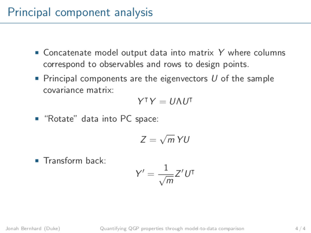
28. Principal component analysis Concatenate model output data into matrix Y where columns correspond to observables and rows to design points. Principal components are the eigenvectors U of the sample covariance matrix: Y Y = UΛU “Rotate” data into PC space: Z = √ m YU Transform back: Y = 1 √ m Z U Jonah Bernhard (Duke) Quantifying QGP properties through model-to-data comparison 4 / 4