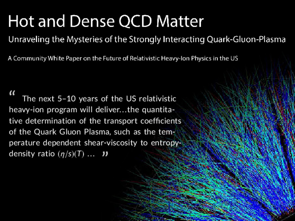
program will deliver...the quantita- tive determination of the transport coefficients of the Quark Gluon Plasma, such as the tem- perature dependent shear-viscosity to entropy- density ratio (η/s)(T) ... ”
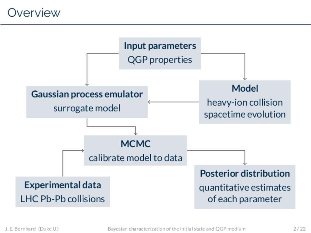
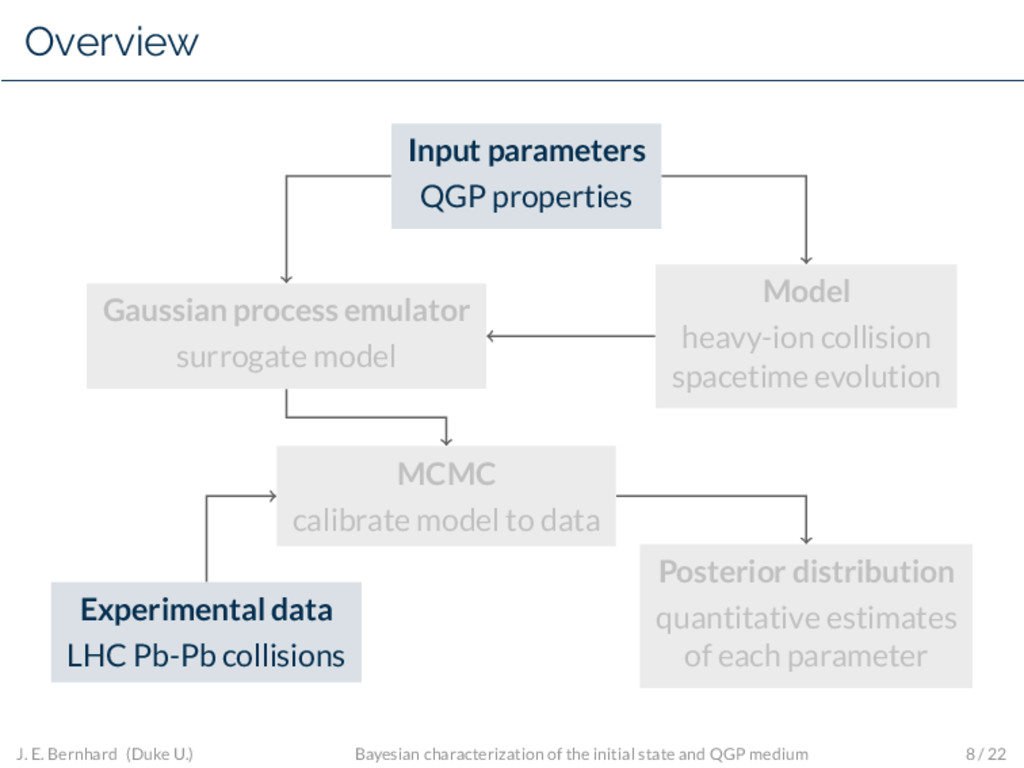
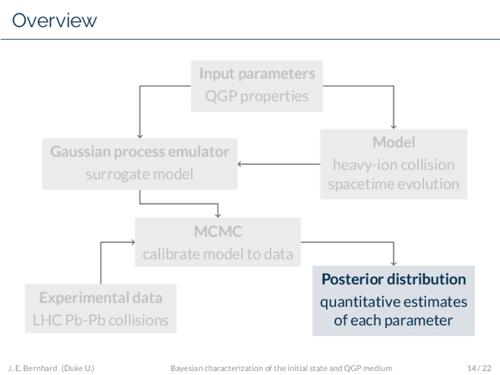
Gaussian process emulator surrogate model MCMC calibrate model to data Posterior distribution quantitative estimates of each parameter Experimental data LHC Pb-Pb collisions J. E. Bernhard (Duke U.) Bayesian characterization of the initial state and QGP medium 2 / 22
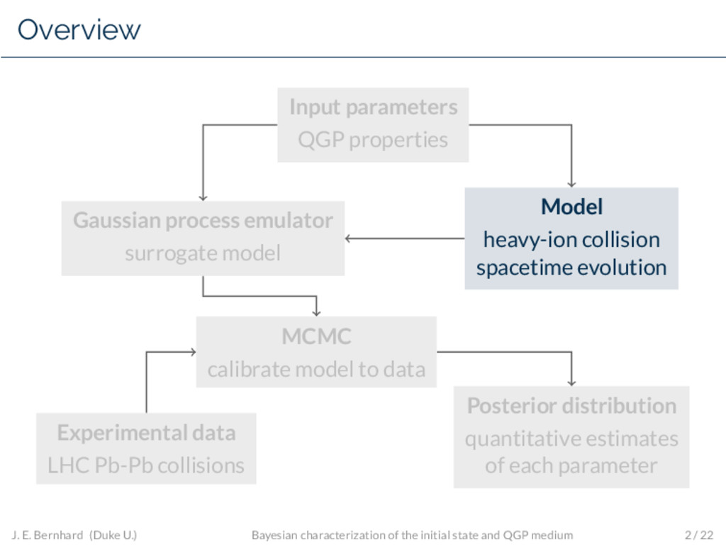
Gaussian process emulator surrogate model MCMC calibrate model to data Posterior distribution quantitative estimates of each parameter Experimental data LHC Pb-Pb collisions J. E. Bernhard (Duke U.) Bayesian characterization of the initial state and QGP medium 2 / 22
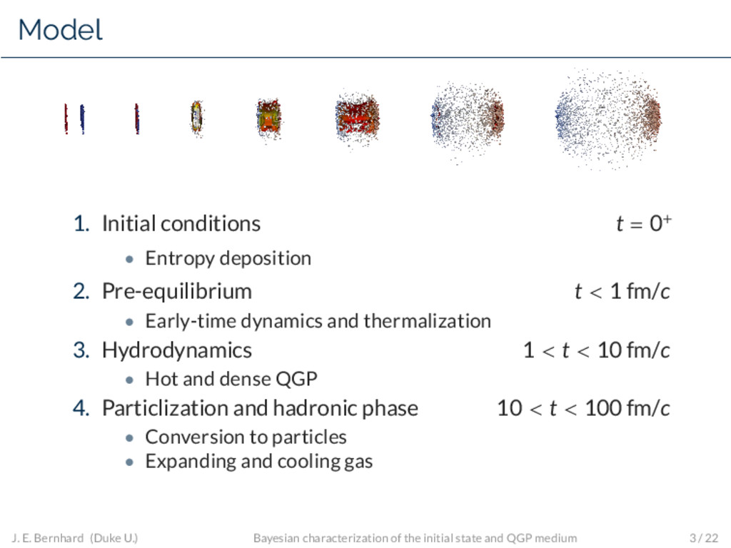
2. Pre-equilibrium t < 1 fm/c • Early-time dynamics and thermalization 3. Hydrodynamics 1 < t < 10 fm/c • Hot and dense QGP 4. Particlization and hadronic phase 10 < t < 100 fm/c • Conversion to particles • Expanding and cooling gas J. E. Bernhard (Duke U.) Bayesian characterization of the initial state and QGP medium 3 / 22
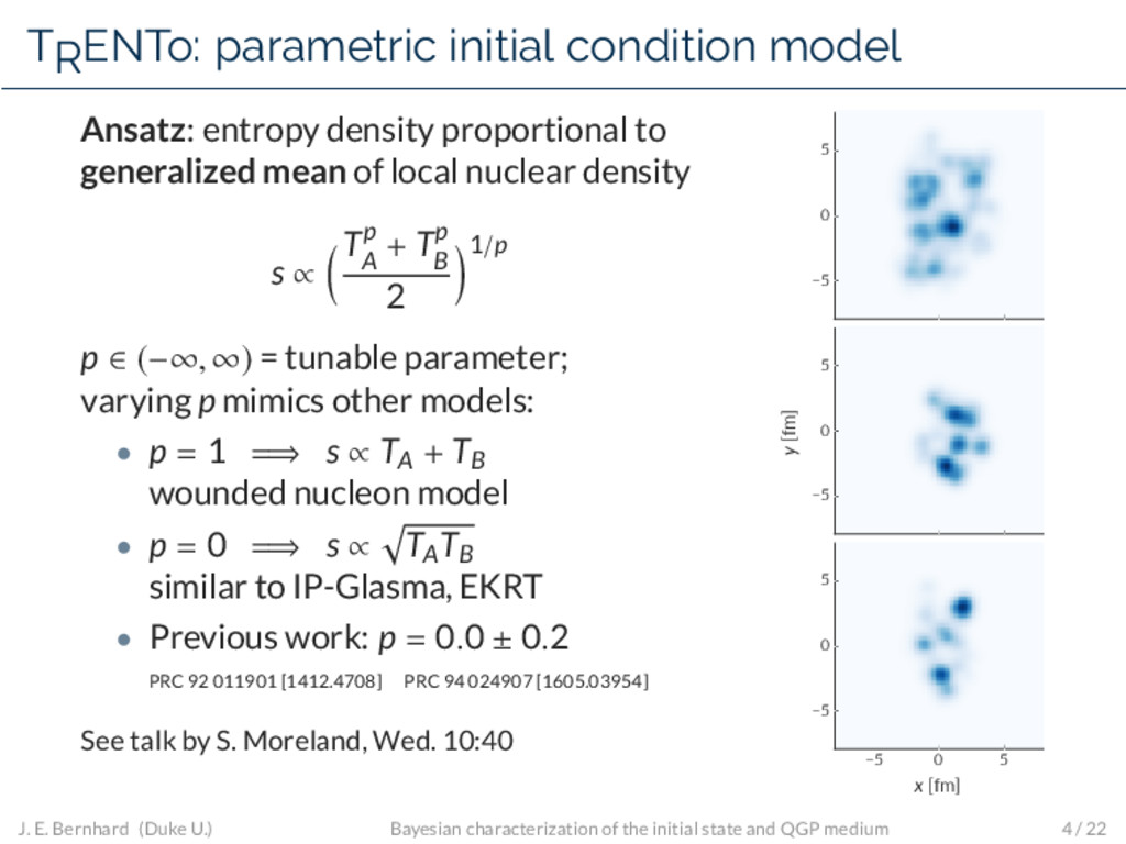
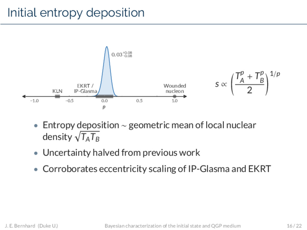
generalized mean of local nuclear density s ∝ Tp A + Tp B 2 1/p p ∈ (−∞, ∞) = tunable parameter; varying p mimics other models: • p = 1 =⇒ s ∝ TA + TB wounded nucleon model • p = 0 =⇒ s ∝ TA TB similar to IP-Glasma, EKRT • Previous work: p = 0.0 ± 0.2 PRC 92 011901 [1412.4708] PRC 94 024907 [1605.03954] See talk by S. Moreland, Wed. 10:40 −5 0 5 −5 0 5 y [fm] −5 0 5 x [fm] −5 0 5 J. E. Bernhard (Duke U.) Bayesian characterization of the initial state and QGP medium 4 / 22
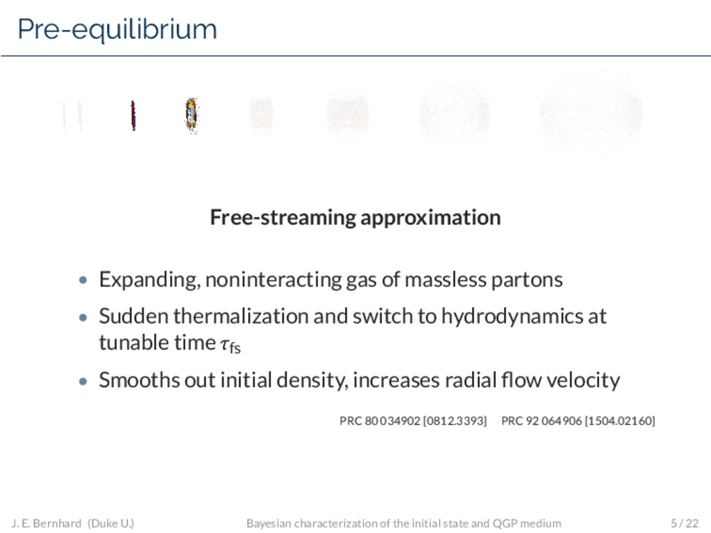
• Sudden thermalization and switch to hydrodynamics at tunable time τfs • Smooths out initial density, increases radial flow velocity PRC 80 034902 [0812.3393] PRC 92 064906 [1504.02160] J. E. Bernhard (Duke U.) Bayesian characterization of the initial state and QGP medium 5 / 22
[1409.8164] • Boost-invariant viscous hydrodynamics • Hybrid equation of state • HRG EOS at low temperature • HOTQCD lattice EOS at high temperature PRD 90 094503 [1407.6387] • Temperature-dependent shear and bulk viscosities J. E. Bernhard (Duke U.) Bayesian characterization of the initial state and QGP medium 6 / 22
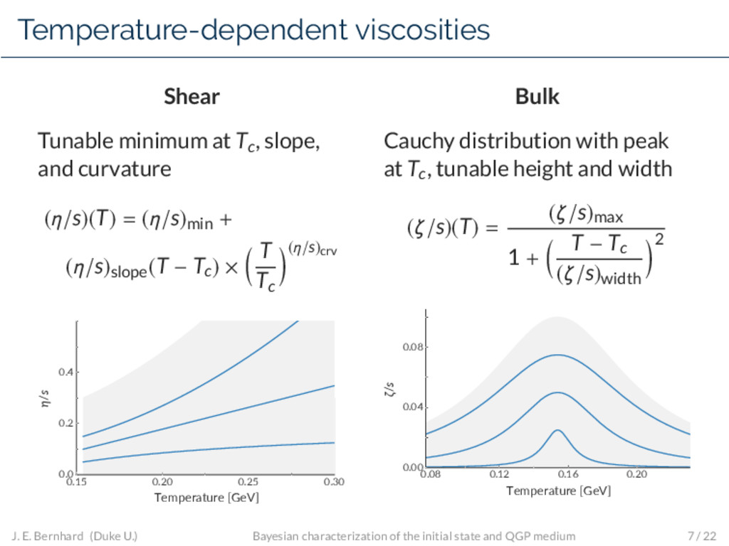
(η/s)(T) = (η/s)min + (η/s)slope(T − Tc) × T Tc (η/s)crv 0.15 0.20 0.25 0.30 Temperature [GeV] 0.0 0.2 0.4 η/s Bulk Cauchy distribution with peak at Tc, tunable height and width (ζ/s)(T) = (ζ/s)max 1 + T − Tc (ζ/s)width 2 0.08 0.12 0.16 0.20 Temperature [GeV] 0.00 0.04 0.08 ζ/s J. E. Bernhard (Duke U.) Bayesian characterization of the initial state and QGP medium 7 / 22
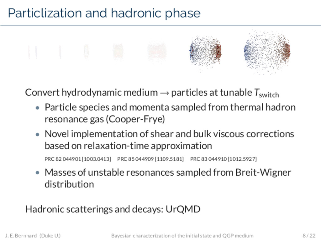
tunable Tswitch • Particle species and momenta sampled from thermal hadron resonance gas (Cooper-Frye) • Novel implementation of shear and bulk viscous corrections based on relaxation-time approximation PRC 82 044901 [1003.0413] PRC 85 044909 [1109.5181] PRC 83 044910 [1012.5927] • Masses of unstable resonances sampled from Breit-Wigner distribution Hadronic scatterings and decays: UrQMD J. E. Bernhard (Duke U.) Bayesian characterization of the initial state and QGP medium 8 / 22
Gaussian process emulator surrogate model MCMC calibrate model to data Posterior distribution quantitative estimates of each parameter Experimental data LHC Pb-Pb collisions J. E. Bernhard (Duke U.) Bayesian characterization of the initial state and QGP medium 8 / 22
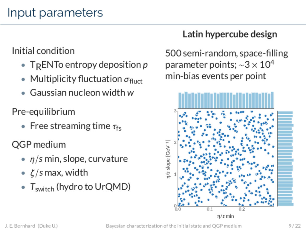
Multiplicity fluctuation σfluct • Gaussian nucleon width w Pre-equilibrium • Free streaming time τfs QGP medium • η/s min, slope, curvature • ζ/s max, width • Tswitch (hydro to UrQMD) Latin hypercube design 500 semi-random, space-filling parameter points; ∼3 × 10⁴ min-bias events per point 0.0 0.1 0.2 η/s min 0 1 2 3 η/s slope [GeV−1] J. E. Bernhard (Duke U.) Bayesian characterization of the initial state and QGP medium 9 / 22
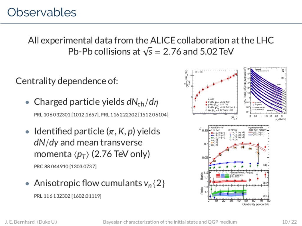
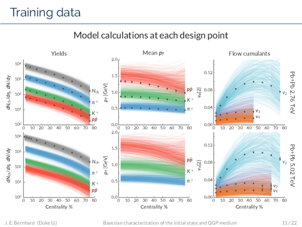
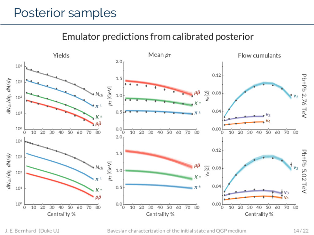
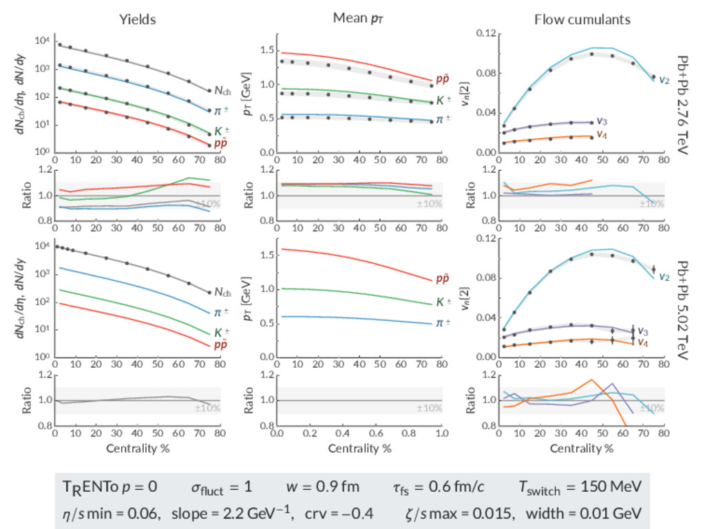
LHC Pb-Pb collisions at √ s = 2.76 and 5.02 TeV Centrality dependence of: • Charged particle yields dNch/dη PRL 106 032301 [1012.1657], PRL 116 222302 [1512.06104] • Identified particle (π, K, p) yields dN/dy and mean transverse momenta pT (2.76 TeV only) PRC 88 044910 [1303.0737] • Anisotropic flow cumulants vn{2} PRL 116 132302 [1602.01119] 〉 part N 〈 0 100 200 300 400 〉 η /d ch N d 〈 〉 part N 〈 2 4 6 8 10 ALICE = 5.02 TeV NN s Pb-Pb, = 5.02 TeV NN s p-Pb, = 2.76 TeV (x1.2) NN s Pb-Pb, = 2.76 TeV (x1.13) NN s pp, | < 0.5 η | ) c (GeV/ T p 0 0.5 1 1.5 2 2.5 3 ] -2 ) c ) [(GeV/ y d T p /(d N 2 ) d T p π 1/(2 ev N 1/ -3 10 -2 10 -1 10 1 10 2 10 3 10 4 10 5 10 6 10 π Range of combined fit 0-5% 80-90% positive negative combined fit individual fit (a) Centrality percentile 0 10 20 30 40 50 60 70 80 n v 0.05 0.1 0.15 5.02 TeV |>1} η ∆ {2, | 2 v |>1} η ∆ {2, | 3 v |>1} η ∆ {2, | 4 v {4} 2 v {6} 2 v {8} 2 v 2.76 TeV |>1} η ∆ {2, | 2 v |>1} η ∆ {2, | 3 v |>1} η ∆ {2, | 4 v {4} 2 v 5.02 TeV, Ref.[27] |>1} η ∆ {2, | 2 v |>1} η ∆ {2, | 3 v ALICE Pb-Pb Hydrodynamics (a) Centrality percentile 0 10 20 30 40 50 60 70 80 Ratio 1 1.1 1.2 /s(T), param1 η /s = 0.20 η (b) Hydrodynamics, Ref.[25] 2 v 3 v 4 v Centrality percentile 0 10 20 30 40 50 60 70 80 Ratio 1 1.1 1.2 (c) J. E. Bernhard (Duke U.) Bayesian characterization of the initial state and QGP medium 10 / 22
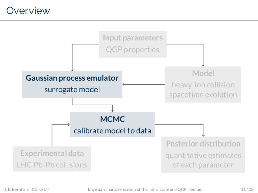
Gaussian process emulator surrogate model MCMC calibrate model to data Posterior distribution quantitative estimates of each parameter Experimental data LHC Pb-Pb collisions J. E. Bernhard (Duke U.) Bayesian characterization of the initial state and QGP medium 11 / 22
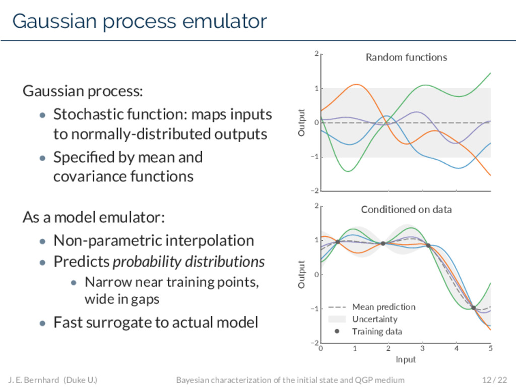
to normally-distributed outputs • Specified by mean and covariance functions As a model emulator: • Non-parametric interpolation • Predicts probability distributions • Narrow near training points, wide in gaps • Fast surrogate to actual model −2 −1 0 1 2 Output Random functions 0 1 2 3 4 5 Input −2 −1 0 1 2 Output Conditioned on data Mean prediction Uncertainty Training data J. E. Bernhard (Duke U.) Bayesian characterization of the initial state and QGP medium 12 / 22
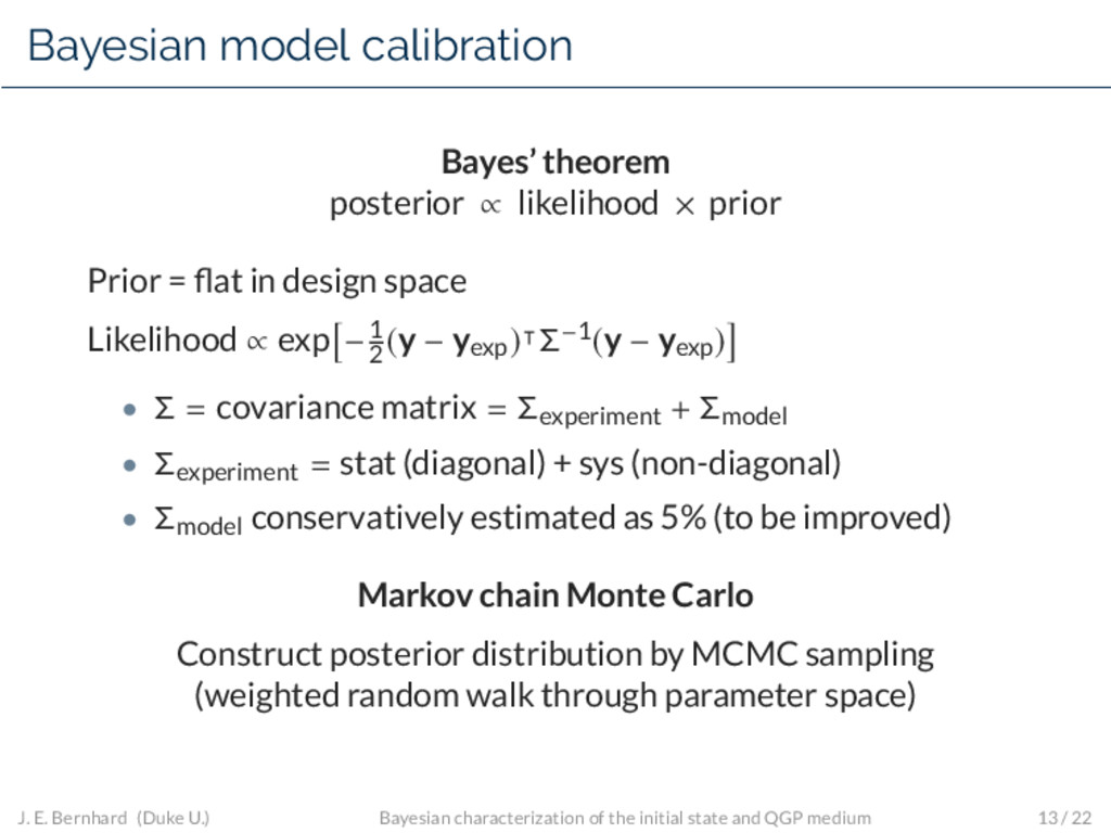
Prior = flat in design space Likelihood ∝ exp −1 2 (y − yexp) Σ−1(y − yexp) • Σ = covariance matrix = Σexperiment + Σmodel • Σexperiment = stat (diagonal) + sys (non-diagonal) • Σmodel conservatively estimated as 5% (to be improved) Markov chain Monte Carlo Construct posterior distribution by MCMC sampling (weighted random walk through parameter space) J. E. Bernhard (Duke U.) Bayesian characterization of the initial state and QGP medium 13 / 22
Gaussian process emulator surrogate model MCMC calibrate model to data Posterior distribution quantitative estimates of each parameter Experimental data LHC Pb-Pb collisions J. E. Bernhard (Duke U.) Bayesian characterization of the initial state and QGP medium 14 / 22
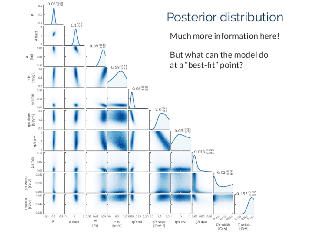
EKRT / IP-Glasma Wounded nucleon 0. 03+0. 08 −0. 08 s ∝ Tp A + Tp B 2 1/p • Entropy deposition ∼ geometric mean of local nuclear density TA TB • Uncertainty halved from previous work • Corroborates eccentricity scaling of IP-Glasma and EKRT J. E. Bernhard (Duke U.) Bayesian characterization of the initial state and QGP medium 16 / 22
T Tc (η/s)crv 0.00 0.15 0.30 η/s min 0. 06+0. 03 −0. 03 0.0 1.5 3.0 η/s slope [GeV−1] 2. 0+1. 0 −0. 8 0.00 0.15 0.30 η/s min −1 0 1 η/s crv 0.0 1.5 3.0 η/s slope [GeV−1] −1 0 1 η/s crv 0. 05+0. 95 −0. 73 0.15 0.20 0.25 0.30 Temperature [GeV] 0.0 0.2 0.4 η/s KSS bound 1/4π Prior range Posterior median 90% credible region • Zero η/s excluded; min consistent with AdS/CFT • Constant η/s excluded • Best constrained T 0.23 GeV • RHIC data could disambiguate slope and curvature J. E. Bernhard (Duke U.) Bayesian characterization of the initial state and QGP medium 17 / 22
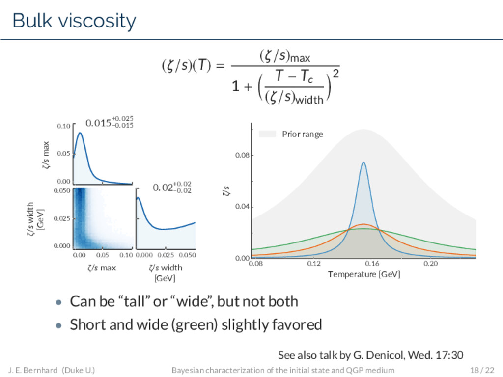
(ζ/s)width 2 0.00 0.05 0.10 ζ/s max 0. 015+0. 025 −0. 015 0.00 0.05 0.10 ζ/s max 0.000 0.025 0.050 ζ/s width [GeV] 0.000 0.025 0.050 ζ/s width [GeV] 0. 02+0. 02 −0. 02 0.08 0.12 0.16 0.20 Temperature [GeV] 0.00 0.04 0.08 ζ/s Prior range • Can be “tall” or “wide”, but not both • Short and wide (green) slightly favored See also talk by G. Denicol, Wed. 17:30 J. E. Bernhard (Duke U.) Bayesian characterization of the initial state and QGP medium 18 / 22
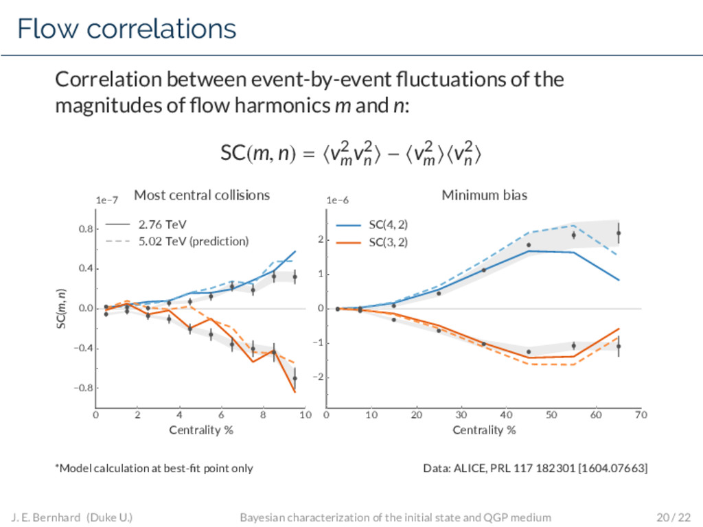
flow harmonics m and n: SC(m, n) = v2 m v2 n − v2 m v2 n 0 2 4 6 8 10 Centrality % −0.8 −0.4 0.0 0.4 0.8 SC(m, n) 1e−7 Most central collisions 2.76 TeV 5.02 TeV (prediction) 0 10 20 30 40 50 60 70 Centrality % −2 −1 0 1 2 1e−6 Minimum bias SC(4, 2) SC(3, 2) *Model calculation at best-fit point only Data: ALICE, PRL 117 182301 [1604.07663] J. E. Bernhard (Duke U.) Bayesian characterization of the initial state and QGP medium 20 / 22
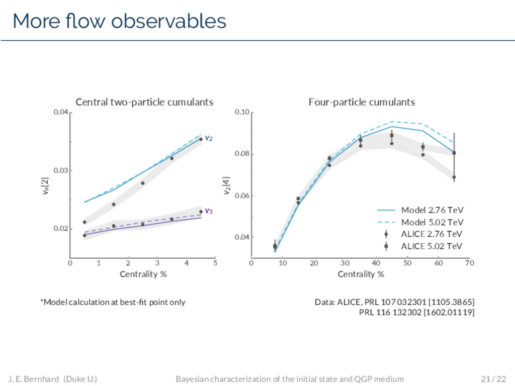
% 0.02 0.03 0.04 vn {2} v2 v3 Central two-particle cumulants 0 10 20 30 40 50 60 70 Centrality % 0.04 0.06 0.08 0.10 v2 {4} Four-particle cumulants Model 2.76 TeV Model 5.02 TeV ALICE 2.76 TeV ALICE 5.02 TeV *Model calculation at best-fit point only Data: ALICE, PRL 107 032301 [1105.3865] PRL 116 132302 [1602.01119] J. E. Bernhard (Duke U.) Bayesian characterization of the initial state and QGP medium 21 / 22
model to diverse experimental data at 2.76 and 5.02 TeV • Constrained initial state entropy deposition, fluctuations, and granularity • Estimated temperature dependence of QGP shear and bulk viscosities • Excluded both zero and constant η/s • Found preference for short, wide ζ/s peak • Include RHIC data to further constrain transport coefficients • Improve uncertainty quantification This project is open source! https://github.com/jbernhard/qm2017 J. E. Bernhard (Duke U.) Bayesian characterization of the initial state and QGP medium 22 / 22
what is the covariance matrix Σ? In general: Σij = cijσiσj where cij = correlation coefficient between observations i, j • Statistical (uncorrelated) uncertainty cij = δij =⇒ Σstat = diag(σ2 i ) • Systematic uncertainty: assume Gaussian correlation function cij = exp − 1 2 xi − xj 100 2 where xi is the centrality % midpoint of observation i J. E. Bernhard (Duke U.) Bayesian characterization of the initial state and QGP medium 2 / 4
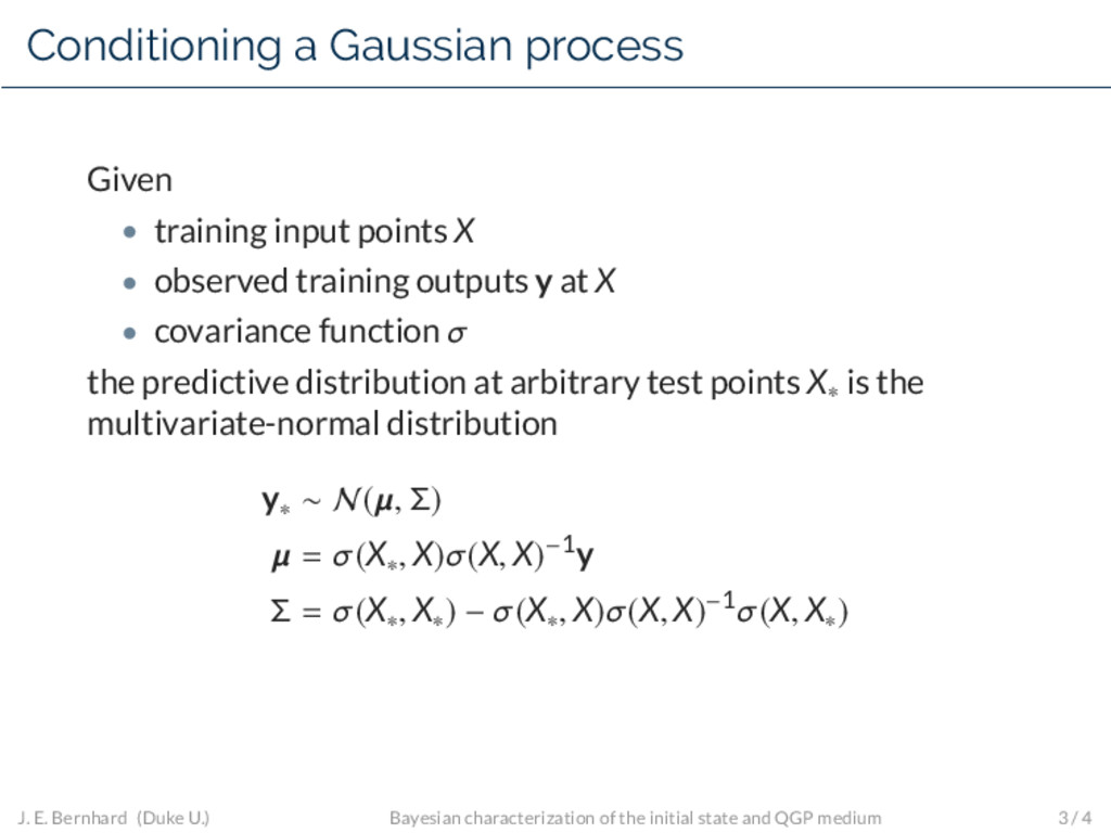
• observed training outputs y at X • covariance function σ the predictive distribution at arbitrary test points X∗ is the multivariate-normal distribution y∗ ∼ N(µ, Σ) µ = σ(X∗ , X)σ(X, X)−1y Σ = σ(X∗ , X∗) − σ(X∗ , X)σ(X, X)−1σ(X, X∗) J. E. Bernhard (Duke U.) Bayesian characterization of the initial state and QGP medium 3 / 4
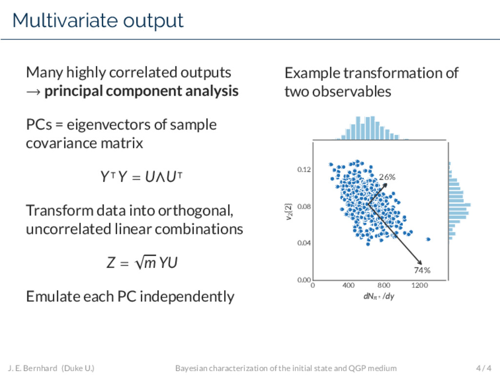
PCs = eigenvectors of sample covariance matrix Y Y = UΛU Transform data into orthogonal, uncorrelated linear combinations Z = √ m YU Emulate each PC independently Example transformation of two observables 0 400 800 1200 dNπ ± /dy 0.00 0.04 0.08 0.12 v2 {2} 74% 26% J. E. Bernhard (Duke U.) Bayesian characterization of the initial state and QGP medium 4 / 4
![Hydrodynamics OSU VISH2+1 PRC 77 064901 [0712.3715] CPC 199 61](https://files.speakerdeck.com/presentations/3f8f030bc5454dcca4bcdbe5addb17d8/slide_7.jpg)