Model-to-data comparison for event-by-event flow distributions: progress and pitfalls

Presented at the workshop "Toward Quantitative Conclusions from Heavy-Ion Collisions", Michigan State University http://nscl.msu.edu/researchers/quark-gluon-plasma.html https://phys.cst.temple.edu/qcd/doc/Quant_Modeling_WP.pdf

Transcript

1. Model-to-data comparison for event-by-event flow distributions: progress and pitfalls Jonah E. Bernhard Steffen A. Bass MSU July 7, 2014
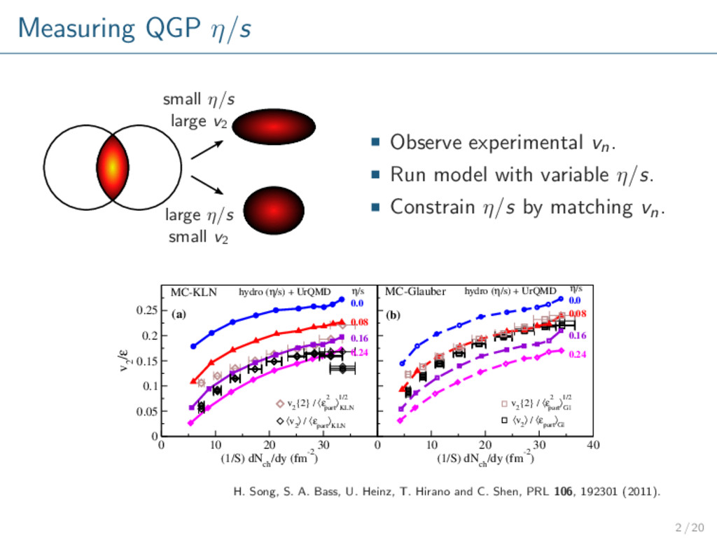
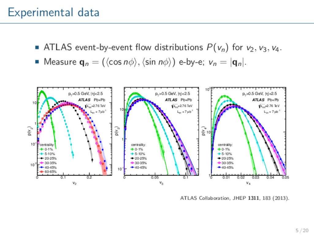
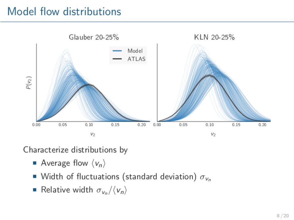
2. Model-to-data comparison 2 v 0 0.1 0.2 ) 2 p(v -2 10 -1 10 1 10 |<2.5 η >0.5 GeV, | T p centrality: 0-1% 5-10% 20-25% 30-35% 40-45% 60-65% ATLAS Pb+Pb =2.76 TeV NN s -1 b µ = 7 int L 3 v 0 0.05 0.1 ) 3 p(v -1 10 1 10 |<2.5 η >0.5 GeV, | T p centrality: 0-1% 5-10% 20-25% 30-35% 40-45% ATLAS Pb+Pb =2.76 TeV NN s -1 b µ = 7 int L 4 v 0 0.01 0.02 0.03 0.04 ) 4 p(v 1 10 2 10 |<2.5 η >0.5 GeV, | T p centrality: 0-1% 5-10% 20-25% 30-35% 40-45% ATLAS Pb+Pb =2.76 TeV NN s -1 b µ = 7 int L 0.05 Model Initial conditions, τ0, η/s, . . . 0.00 0.05 0.10 0.15 0.20 v2 P(v2 ) Glauber 20-25% Model ATLAS 0.00 0.05 0.10 0.15 0.20 v2 KLN 20-25% 1 / 20
3. Measuring QGP η/s small η/s large v2 large η/s small v2 Observe experimental vn. Run model with variable η/s. Constrain η/s by matching vn. 0 10 20 30 (1/S) dN ch /dy (fm-2 ) 0 0.05 0.1 0.15 0.2 0.25 v 2 /ε 0 10 20 30 40 (1/S) dN ch /dy (fm-2 ) hydro (η/s) + UrQMD hydro (η/s) + UrQMD MC-Glauber MC-KLN 0.0 0.08 0.16 0.24 0.0 0.08 0.16 0.24 η/s η/s v 2 {2} / 〈ε2 part 〉1/2 Gl (a) (b) 〈v 2 〉 / 〈ε part 〉 Gl v 2 {2} / 〈ε2 part 〉1/2 KLN 〈v 2 〉 / 〈ε part 〉 KLN H. Song, S. A. Bass, U. Heinz, T. Hirano and C. Shen, PRL 106, 192301 (2011). 2 / 20
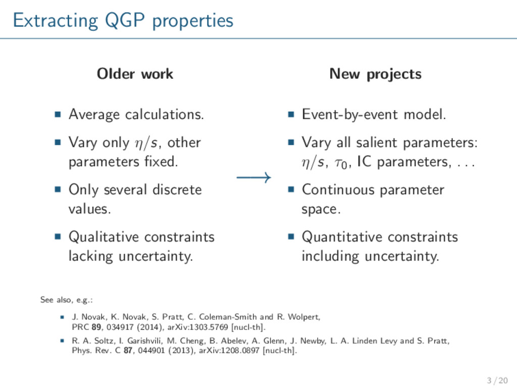
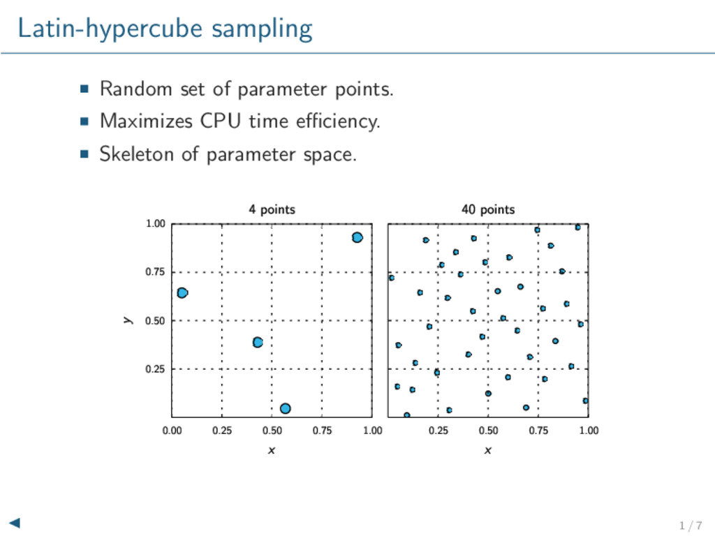
4. Extracting QGP properties Older work Average calculations. Vary only η/s, other parameters fixed. Only several discrete values. Qualitative constraints lacking uncertainty. New projects Event-by-event model. Vary all salient parameters: η/s, τ0, IC parameters, . . . Continuous parameter space. Quantitative constraints including uncertainty. See also, e.g.: J. Novak, K. Novak, S. Pratt, C. Coleman-Smith and R. Wolpert, PRC 89, 034917 (2014), arXiv:1303.5769 [nucl-th]. R. A. Soltz, I. Garishvili, M. Cheng, B. Abelev, A. Glenn, J. Newby, L. A. Linden Levy and S. Pratt, Phys. Rev. C 87, 044901 (2013), arXiv:1208.0897 [nucl-th]. −→ 3 / 20
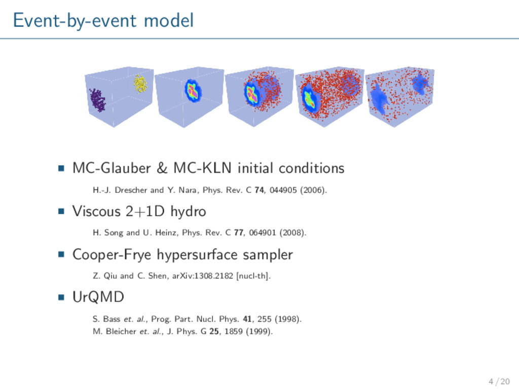
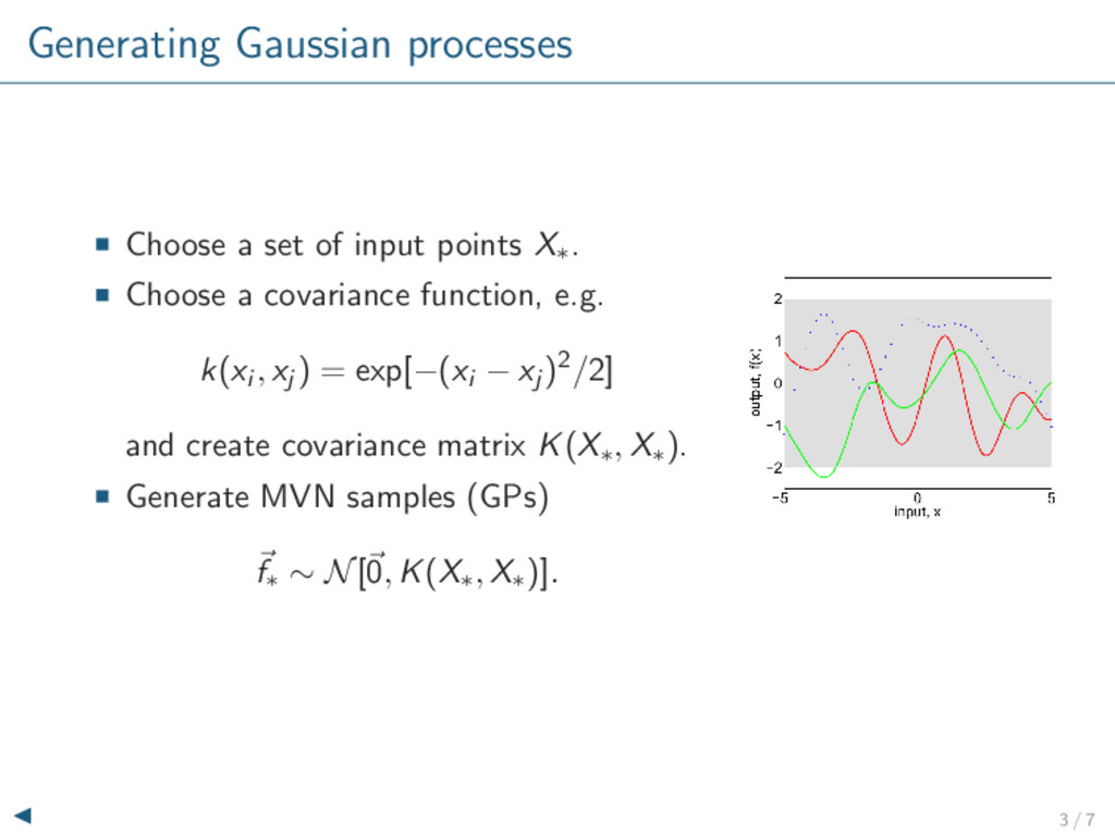
5. Event-by-event model MC-Glauber & MC-KLN initial conditions H.-J. Drescher and Y. Nara, Phys. Rev. C 74, 044905 (2006). Viscous 2+1D hydro H. Song and U. Heinz, Phys. Rev. C 77, 064901 (2008). Cooper-Frye hypersurface sampler Z. Qiu and C. Shen, arXiv:1308.2182 [nucl-th]. UrQMD S. Bass et. al., Prog. Part. Nucl. Phys. 41, 255 (1998). M. Bleicher et. al., J. Phys. G 25, 1859 (1999). 4 / 20
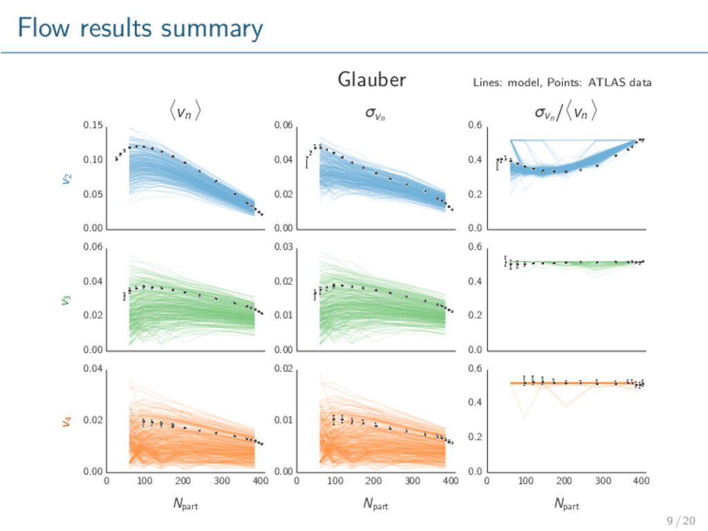
6. Experimental data ATLAS event-by-event flow distributions P(vn) for v2, v3, v4. Measure qn = ( cos nφ , sin nφ ) e-by-e; vn = |qn|. 2 v 0 0.1 0.2 ) 2 p(v -2 10 -1 10 1 10 |<2.5 η >0.5 GeV, | T p centrality: 0-1% 5-10% 20-25% 30-35% 40-45% 60-65% ATLAS Pb+Pb =2.76 TeV NN s -1 b µ = 7 int L 3 v 0 0.05 0.1 ) 3 p(v -1 10 1 10 |<2.5 η >0.5 GeV, | T p centrality: 0-1% 5-10% 20-25% 30-35% 40-45% ATLAS Pb+Pb =2.76 TeV NN s -1 b µ = 7 int L 4 v 0 0.01 0.02 0.03 0.04 ) 4 p(v 1 10 2 10 |<2.5 η >0.5 GeV, | T p centrality: 0-1% 5-10% 20-25% 30-35% 40-45% ATLAS Pb+Pb =2.76 TeV NN s -1 b µ = 7 int L 0.05 ATLAS Collaboration, JHEP 1311, 183 (2013). 5 / 20
7. Computer experiment design Minimum 1000 events per set of input parameters and centrality class. 256 parameter points, varying 5 parameters simultaneously Normalization IC-specific parameter Thermalization time τ0 Viscosity η/s Shear relaxation time τΠ 6 centrality classes 0–5%, 10–15%, . . . , 50–55%. 2 initial condition models. 1000 × 256 × 6 × 2 > 3 million events 3 million hours ∼ 350 years 6 / 20
8. Open Science Grid usage CPU hours per day 250,000 red = Me Completed KLN design (1.5 million events) in two weeks. ∼4 million total → 0.55 µb−1 (ATLAS: 7 µb−1) Extensible to other projects. 7 / 20
9. Model flow distributions 0.00 0.05 0.10 0.15 0.20 v2 P(v2 ) Glauber 20-25% Model ATLAS 0.00 0.05 0.10 0.15 0.20 v2 KLN 20-25% Characterize distributions by Average flow vn Width of fluctuations (standard deviation) σvn Relative width σvn / vn 8 / 20
10. Flow results summary Glauber Lines: model, Points: ATLAS data 0.00 0.05 0.10 0.15 v2 ­ vn ® 0.00 0.02 0.04 0.06 σvn 0.0 0.2 0.4 0.6 σvn / ­ vn ® 0.00 0.02 0.04 0.06 v3 0.00 0.01 0.02 0.03 0.0 0.2 0.4 0.6 0 100 200 300 400 Npart 0.00 0.02 0.04 v4 0 100 200 300 400 Npart 0.00 0.01 0.02 0 100 200 300 400 Npart 0.0 0.2 0.4 0.6 9 / 20
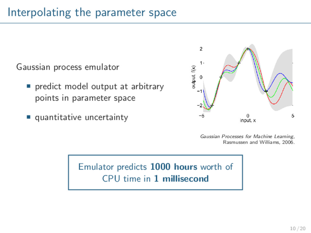
11. Interpolating the parameter space Gaussian process emulator predict model output at arbitrary points in parameter space quantitative uncertainty Gaussian Processes for Machine Learning, Rasmussen and Williams, 2006. Emulator predicts 1000 hours worth of CPU time in 1 millisecond 10 / 20
12. Emulator predictions Glauber 0 100 200 300 400 Npart 0.00 0.04 0.08 0.12 η/s 0.04 0.08 0.12 0.16 ­ vn ® 0 100 200 300 400 Npart 0.00 0.02 0.04 σvn 0 100 200 300 400 Npart 0.0 0.2 0.4 0.6 σvn / ­ vn ® Colors v2 v3 v4 Lines η/s = 0.04, 0.08, 0.12, 0.16, top to bottom Points ATLAS data 11 / 20
13. Emulator predictions Glauber 20–25% centrality 0.00 0.08 0.16 0.24 η/s 0.00 0.04 0.08 0.12 α 0.24 0.18 0.12 0.06 ­ vn ® 0.00 0.08 0.16 0.24 η/s 0.00 0.02 0.04 σvn 0.00 0.08 0.16 0.24 η/s 0.0 0.2 0.4 0.6 σvn / ­ vn ® Colors v2 v3 v4 Lines Glauber α = 0.06, 0.12, 0.18, 0.24, bottom to top Bands ATLAS measurements 12 / 20
14. Flow results summary KLN 0.00 0.05 0.10 0.15 v2 ­ vn ® 0.00 0.02 0.04 0.06 σvn 0.0 0.2 0.4 0.6 σvn / ­ vn ® 0.00 0.02 0.04 0.06 v3 0.00 0.01 0.02 0.03 0.0 0.2 0.4 0.6 0 100 200 300 400 Npart 0.00 0.02 0.04 v4 0 100 200 300 400 Npart 0.00 0.01 0.02 0 100 200 300 400 Npart 0.0 0.2 0.4 0.6 13 / 20
15. Emulator predictions KLN 0 100 200 300 400 Npart 0.00 0.04 0.08 0.12 η/s 0.12 0.16 0.20 0.24 ­ vn ® 0 100 200 300 400 Npart 0.00 0.02 0.04 σvn 0 100 200 300 400 Npart 0.0 0.2 0.4 0.6 σvn / ­ vn ® Colors v2 v3 v4 Lines η/s = 0.12, 0.16, 0.20, 0.24, top to bottom Points ATLAS data 14 / 20
16. Emulator predictions KLN 20–25% centrality 0.00 0.08 0.16 0.24 η/s 0.00 0.04 0.08 0.12 λ 0.25 0.20 0.15 0.10 ­ vn ® 0.00 0.08 0.16 0.24 η/s 0.00 0.02 0.04 σvn 0.00 0.08 0.16 0.24 η/s 0.0 0.2 0.4 0.6 σvn / ­ vn ® Colors v2 v3 v4 Lines KLN λ = 0.10, 0.15, 0.20, 0.25, bottom to top Bands ATLAS measurements 15 / 20
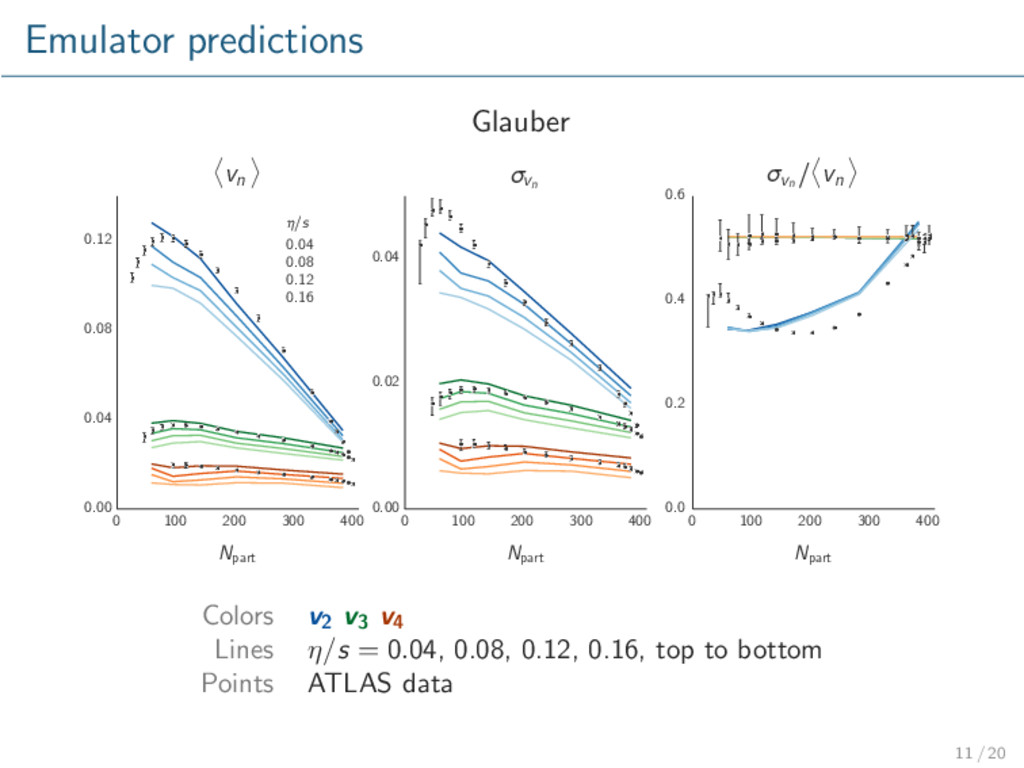
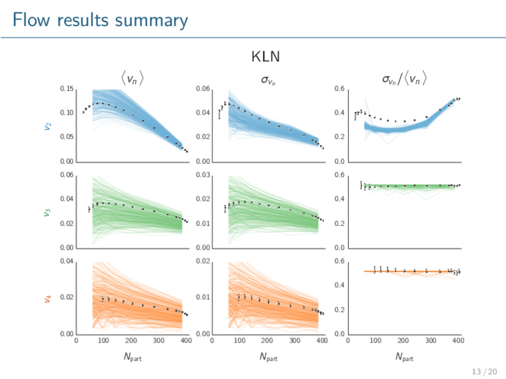
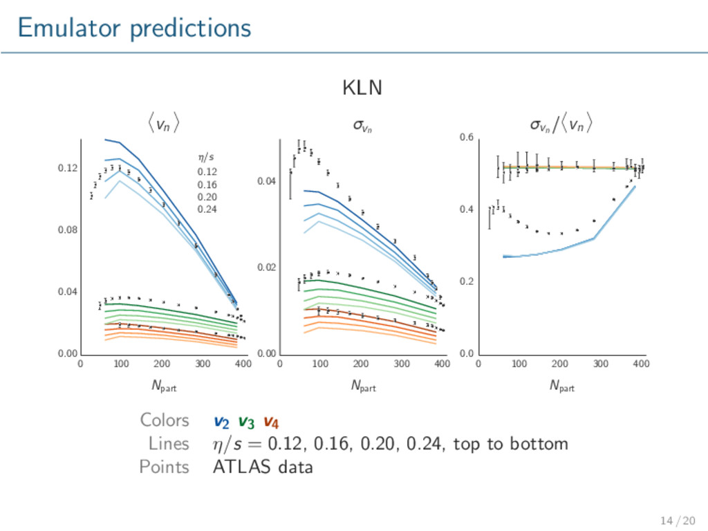
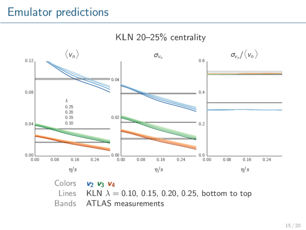
17. Intermission Framework for massive event-by-event model-to-data comparison. Systematic model validation / exclusion. Glauber qualitatively describes data. KLN does not. Repeat with more advanced models, especially initial conditions. Rigorously calibrate model to data → extract optimal parameters with uncertainty. Consider other observables, e.g. identified particle spectra, dNch/dy. Solve the finite-multiplicity problem. 16 / 20
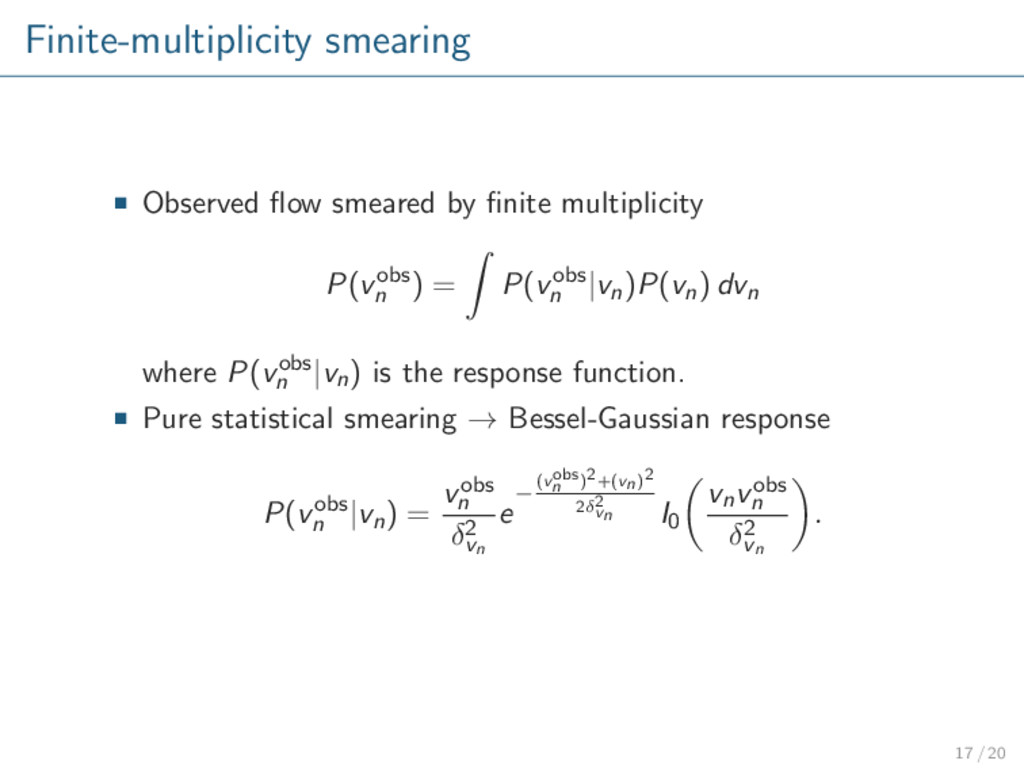
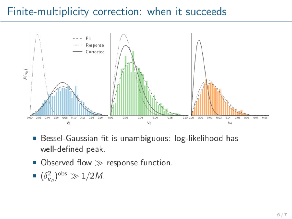
18. Finite-multiplicity smearing Observed flow smeared by finite multiplicity P(vobs n ) = P(vobs n |vn)P(vn) dvn where P(vobs n |vn) is the response function. Pure statistical smearing → Bessel-Gaussian response P(vobs n |vn) = vobs n δ2 vn e −(vobs n )2+(vn)2 2δ2 vn I0 vnvobs n δ2 vn . 17 / 20
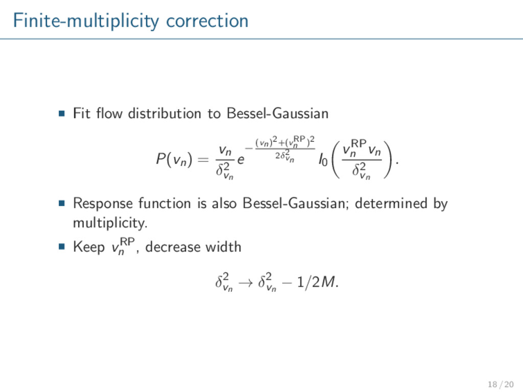
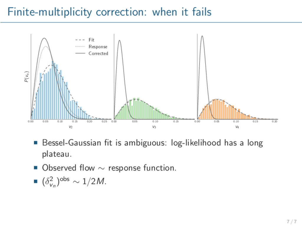
19. Finite-multiplicity correction Fit flow distribution to Bessel-Gaussian P(vn) = vn δ2 vn e −(vn)2+(vRP n )2 2δ2 vn I0 vRP n vn δ2 vn . Response function is also Bessel-Gaussian; determined by multiplicity. Keep vRP n , decrease width δ2 vn → δ2 vn − 1/2M. 18 / 20
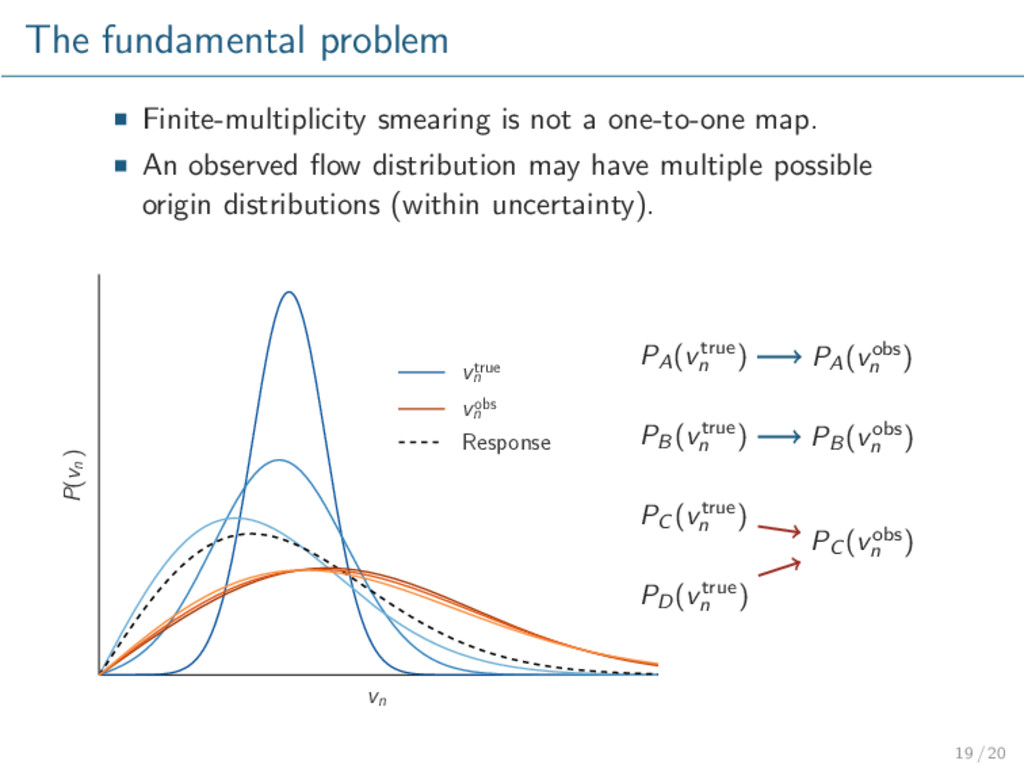
20. The fundamental problem Finite-multiplicity smearing is not a one-to-one map. An observed flow distribution may have multiple possible origin distributions (within uncertainty). vn P(vn ) vtrue n vobs n Response PA (vtrue n ) PB (vtrue n ) PC (vtrue n ) PD (vtrue n ) PA (vobs n ) PB (vobs n ) PC (vobs n ) 19 / 20
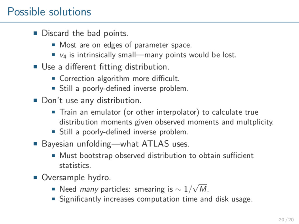
21. Possible solutions Discard the bad points. Most are on edges of parameter space. v4 is intrinsically small—many points would be lost. Use a different fitting distribution. Correction algorithm more difficult. Still a poorly-defined inverse problem. Don’t use any distribution. Train an emulator (or other interpolator) to calculate true distribution moments given observed moments and multplicity. Still a poorly-defined inverse problem. Bayesian unfolding—what ATLAS uses. Must bootstrap observed distribution to obtain sufficient statistics. Oversample hydro. Need many particles: smearing is ∼ 1/ √ M. Significantly increases computation time and disk usage. 20 / 20
22. backup slides
23. Latin-hypercube sampling Random set of parameter points. Maximizes CPU time efficiency. Skeleton of parameter space. 0.00 0.25 0.50 0.75 1.00 x 0.25 0.50 0.75 1.00 y 4 points 0.25 0.50 0.75 1.00 x 40 points 1 / 7
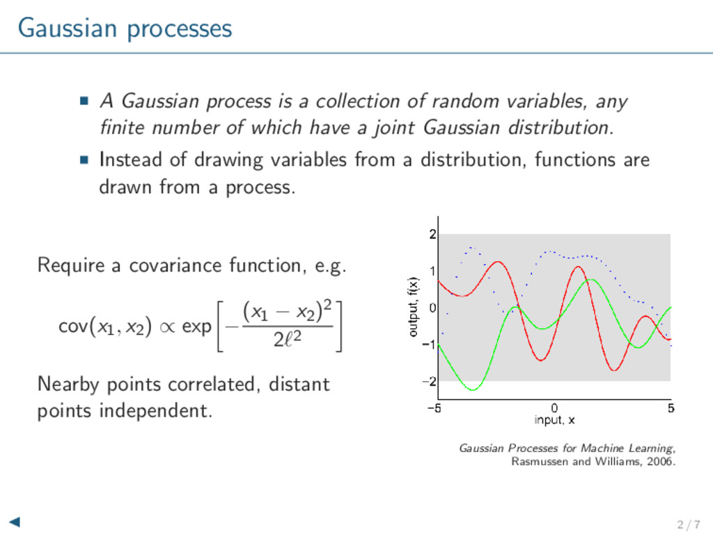
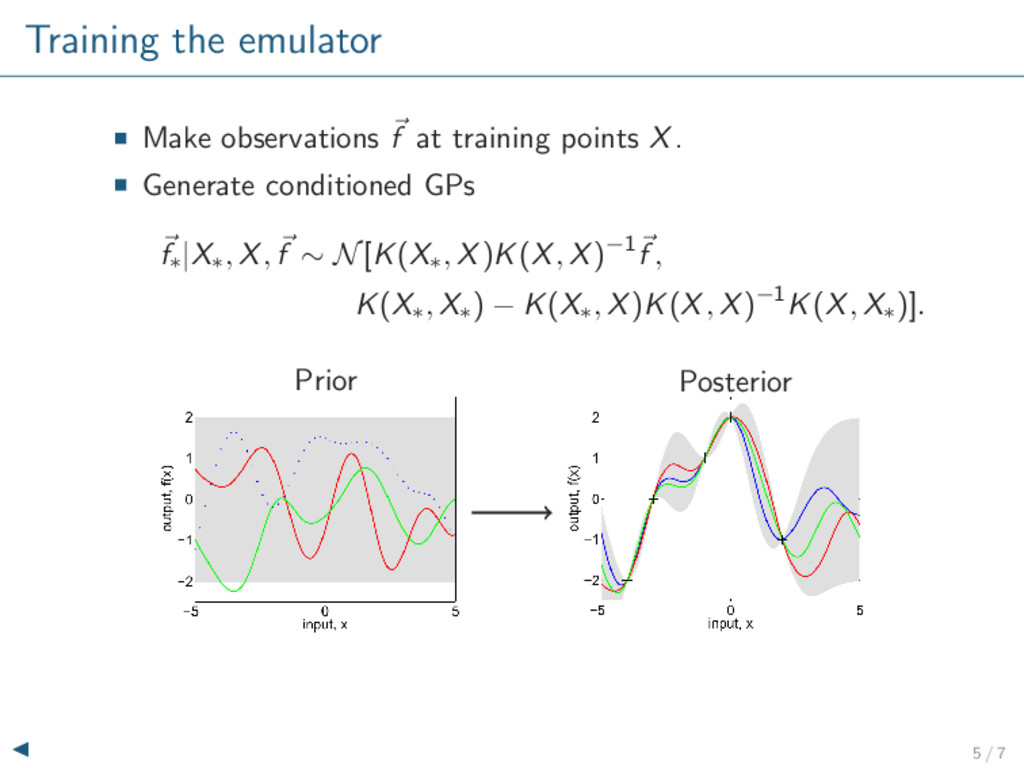
24. Gaussian processes A Gaussian process is a collection of random variables, any finite number of which have a joint Gaussian distribution. Instead of drawing variables from a distribution, functions are drawn from a process. Require a covariance function, e.g. cov(x1, x2) ∝ exp − (x1 − x2)2 2 2 Nearby points correlated, distant points independent. Gaussian Processes for Machine Learning, Rasmussen and Williams, 2006. 2 / 7
25. Generating Gaussian processes Choose a set of input points X∗. Choose a covariance function, e.g. k(xi , xj ) = exp[−(xi − xj )2/2] and create covariance matrix K(X∗, X∗). Generate MVN samples (GPs) f∗ ∼ N[0, K(X∗, X∗)]. 3 / 7
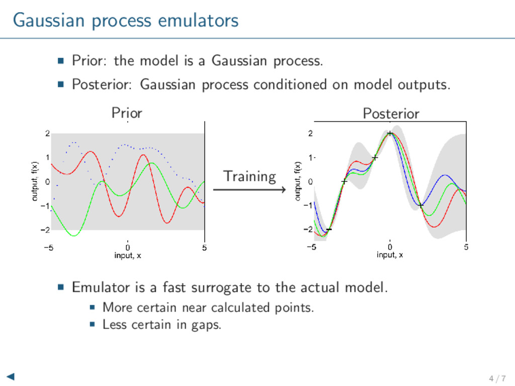
26. Gaussian process emulators Prior: the model is a Gaussian process. Posterior: Gaussian process conditioned on model outputs. Training Prior Posterior Emulator is a fast surrogate to the actual model. More certain near calculated points. Less certain in gaps. 4 / 7
27. Training the emulator Make observations f at training points X. Generate conditioned GPs f∗|X∗, X, f ∼ N[K(X∗, X)K(X, X)−1f , K(X∗, X∗) − K(X∗, X)K(X, X)−1K(X, X∗)]. Prior Posterior 5 / 7
28. Finite-multiplicity correction: when it succeeds 0.00 0.02 0.04 0.06 0.08 0.10 0.12 0.14 0.16 v2 P(vn ) Fit Response Corrected 0.00 0.02 0.04 0.06 0.08 0.10 v3 0.00 0.01 0.02 0.03 0.04 0.05 0.06 0.07 0.08 v4 Bessel-Gaussian fit is unambiguous: log-likelihood has well-defined peak. Observed flow response function. (δ2 vn )obs 1/2M. 6 / 7
29. Finite-multiplicity correction: when it fails 0.00 0.05 0.10 0.15 0.20 0.25 v2 P(vn ) Fit Response Corrected 0.00 0.05 0.10 0.15 v3 0.00 0.05 0.10 0.15 0.20 v4 Bessel-Gaussian fit is ambiguous: log-likelihood has a long plateau. Observed flow ∼ response function. (δ2 vn )obs ∼ 1/2M. 7 / 7