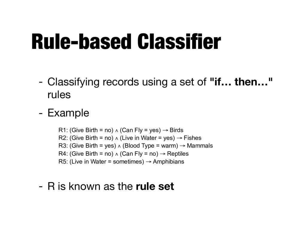
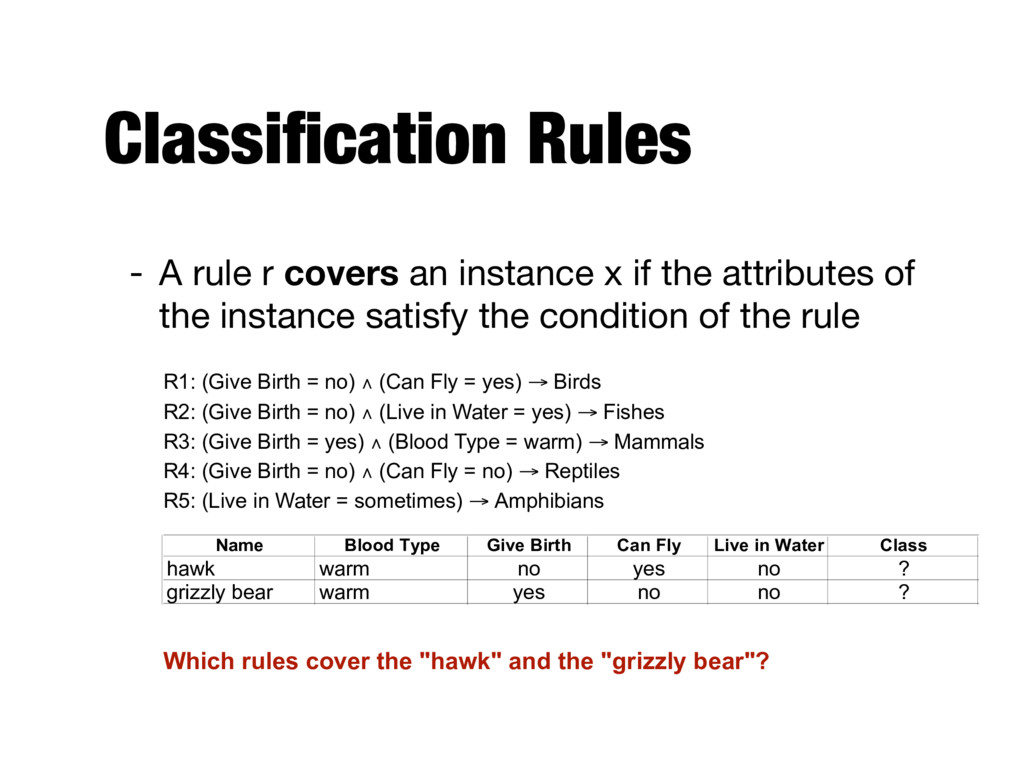
if the attributes of the instance satisfy the condition of the rule R1: (Give Birth = no) ∧ (Can Fly = yes) → Birds R2: (Give Birth = no) ∧ (Live in Water = yes) → Fishes R3: (Give Birth = yes) ∧ (Blood Type = warm) → Mammals R4: (Give Birth = no) ∧ (Can Fly = no) → Reptiles R5: (Live in Water = sometimes) → Amphibians Which rules cover the "hawk" and the "grizzly bear"? Name Blood Type Give Birth Can Fly Live in Water Class hawk warm no yes no ? grizzly bear warm yes no no ?
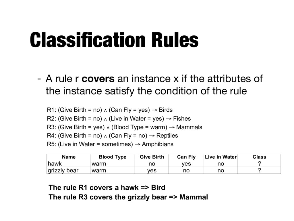
if the attributes of the instance satisfy the condition of the rule R1: (Give Birth = no) ∧ (Can Fly = yes) → Birds R2: (Give Birth = no) ∧ (Live in Water = yes) → Fishes R3: (Give Birth = yes) ∧ (Blood Type = warm) → Mammals R4: (Give Birth = no) ∧ (Can Fly = no) → Reptiles R5: (Live in Water = sometimes) → Amphibians The rule R1 covers a hawk => Bird The rule R3 covers the grizzly bear => Mammal Name Blood Type Give Birth Can Fly Live in Water Class hawk warm no yes no ? grizzly bear warm yes no no ?
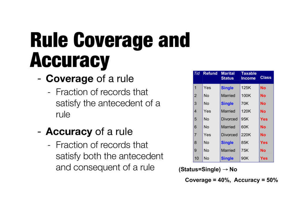
Fraction of records that satisfy the antecedent of a rule - Accuracy of a rule - Fraction of records that satisfy both the antecedent and consequent of a rule Tid Refund Marital Status Taxable Income Class 1 Yes Single 125K No 2 No Married 100K No 3 No Single 70K No 4 Yes Married 120K No 5 No Divorced 95K Yes 6 No Married 60K No 7 Yes Divorced 220K No 8 No Single 85K Yes 9 No Married 75K No 10 No Single 90K Yes 10 (Status=Single) → No Coverage = 40%, Accuracy = 50%
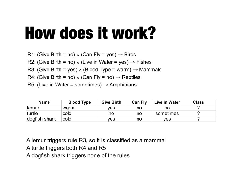
(Can Fly = yes) → Birds R2: (Give Birth = no) ∧ (Live in Water = yes) → Fishes R3: (Give Birth = yes) ∧ (Blood Type = warm) → Mammals R4: (Give Birth = no) ∧ (Can Fly = no) → Reptiles R5: (Live in Water = sometimes) → Amphibians A lemur triggers rule R3, so it is classified as a mammal A turtle triggers both R4 and R5 A dogfish shark triggers none of the rules Name Blood Type Give Birth Can Fly Live in Water Class lemur warm yes no no ? turtle cold no no sometimes ? dogfish shark cold yes no yes ?
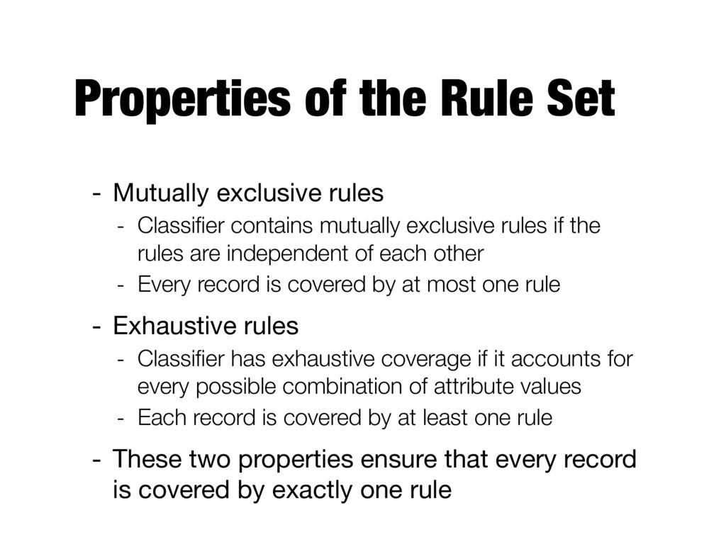
Classifier contains mutually exclusive rules if the rules are independent of each other - Every record is covered by at most one rule - Exhaustive rules - Classifier has exhaustive coverage if it accounts for every possible combination of attribute values - Each record is covered by at least one rule - These two properties ensure that every record is covered by exactly one rule
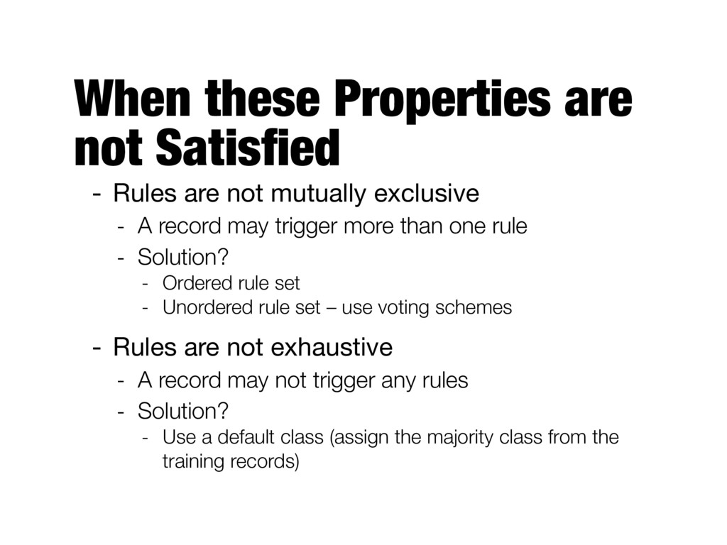
mutually exclusive - A record may trigger more than one rule - Solution? - Ordered rule set - Unordered rule set – use voting schemes - Rules are not exhaustive - A record may not trigger any rules - Solution? - Use a default class (assign the majority class from the training records)
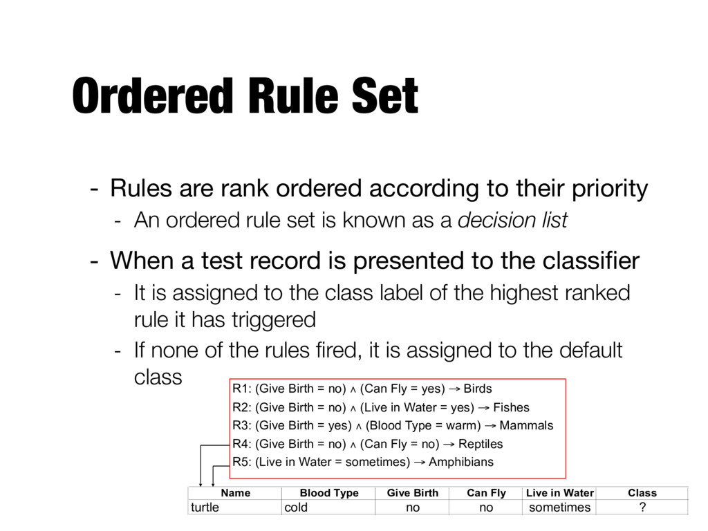
their priority - An ordered rule set is known as a decision list - When a test record is presented to the classifier - It is assigned to the class label of the highest ranked rule it has triggered - If none of the rules fired, it is assigned to the default class R1: (Give Birth = no) ∧ (Can Fly = yes) → Birds R2: (Give Birth = no) ∧ (Live in Water = yes) → Fishes R3: (Give Birth = yes) ∧ (Blood Type = warm) → Mammals R4: (Give Birth = no) ∧ (Can Fly = no) → Reptiles R5: (Live in Water = sometimes) → Amphibians Name Blood Type Give Birth Can Fly Live in Water Class turtle cold no no sometimes ?
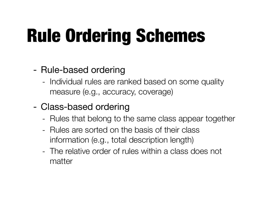
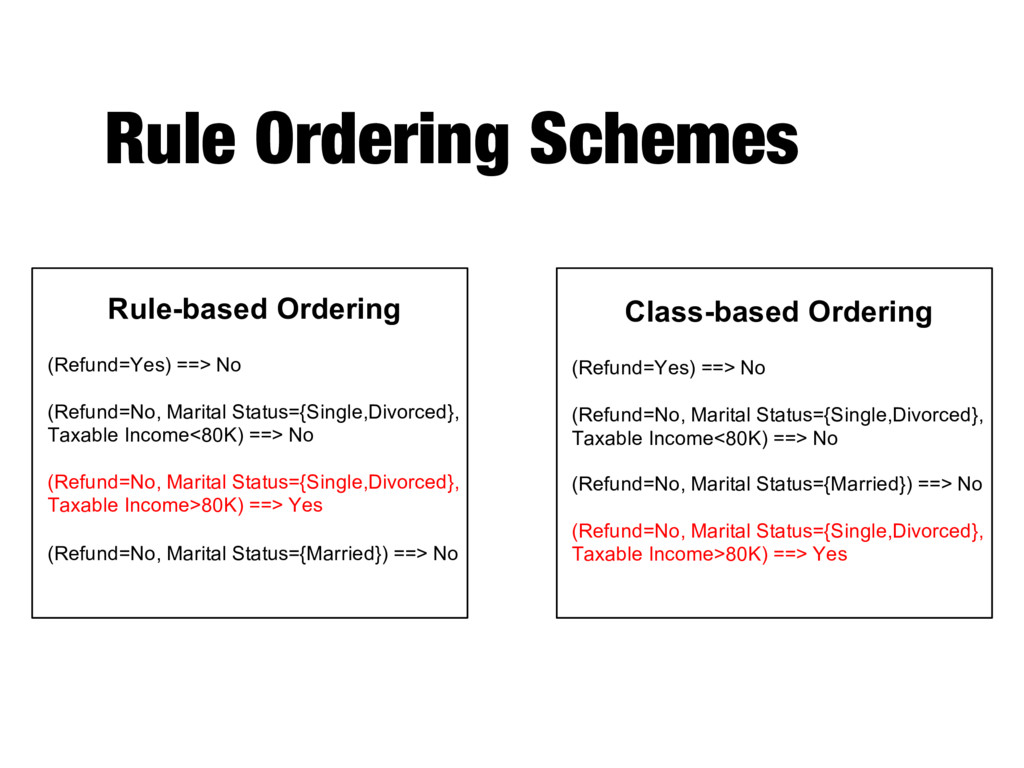
ranked based on some quality measure (e.g., accuracy, coverage) - Class-based ordering - Rules that belong to the same class appear together - Rules are sorted on the basis of their class information (e.g., total description length) - The relative order of rules within a class does not matter
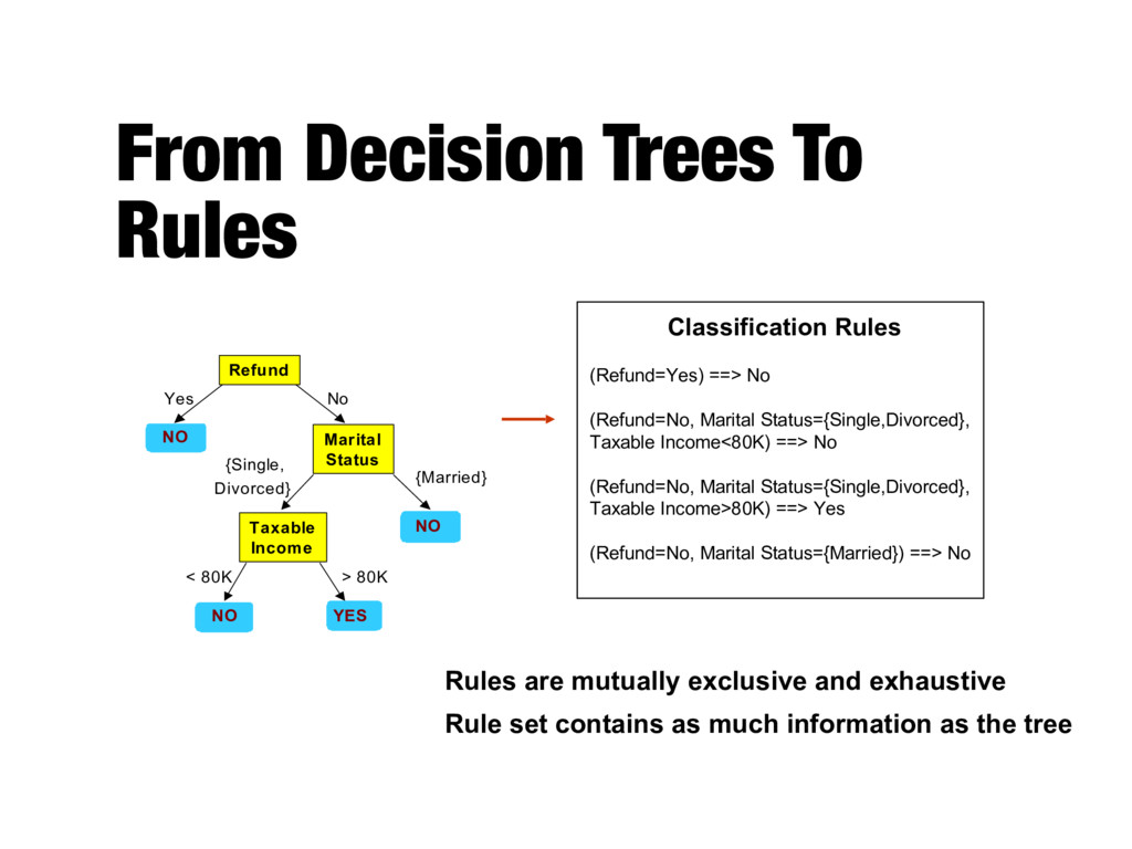
NO NO NO Yes No {Married} {Single, Divorced} < 80K > 80K Taxable Income Marital Status Refund Classification Rules (Refund=Yes) ==> No (Refund=No, Marital Status={Single,Divorced}, Taxable Income<80K) ==> No (Refund=No, Marital Status={Single,Divorced}, Taxable Income>80K) ==> Yes (Refund=No, Marital Status={Married}) ==> No Rules are mutually exclusive and exhaustive Rule set contains as much information as the tree
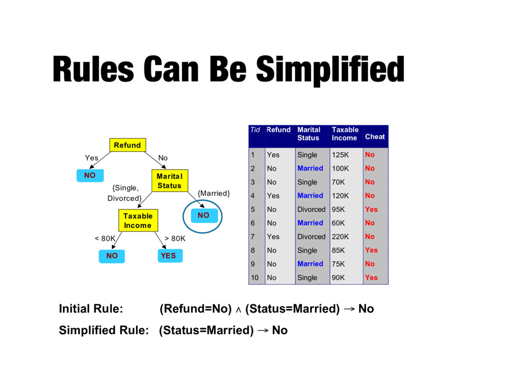
NO NO Yes No {Married} {Single, Divorced} < 80K > 80K Taxable Income Marital Status Refund Tid Refund Marital Status Taxable Income Cheat 1 Yes Single 125K No 2 No Married 100K No 3 No Single 70K No 4 Yes Married 120K No 5 No Divorced 95K Yes 6 No Married 60K No 7 Yes Divorced 220K No 8 No Single 85K Yes 9 No Married 75K No 10 No Single 90K Yes 10 Initial Rule: (Refund=No) ∧ (Status=Married) → No Simplified Rule: (Status=Married) → No
decision tree - Generally used to produce descriptive models that are easy to interpret, but gives comparable performance to decision tree classifiers - The class-based ordering approach is well suited for handling data sets with imbalanced class distributions
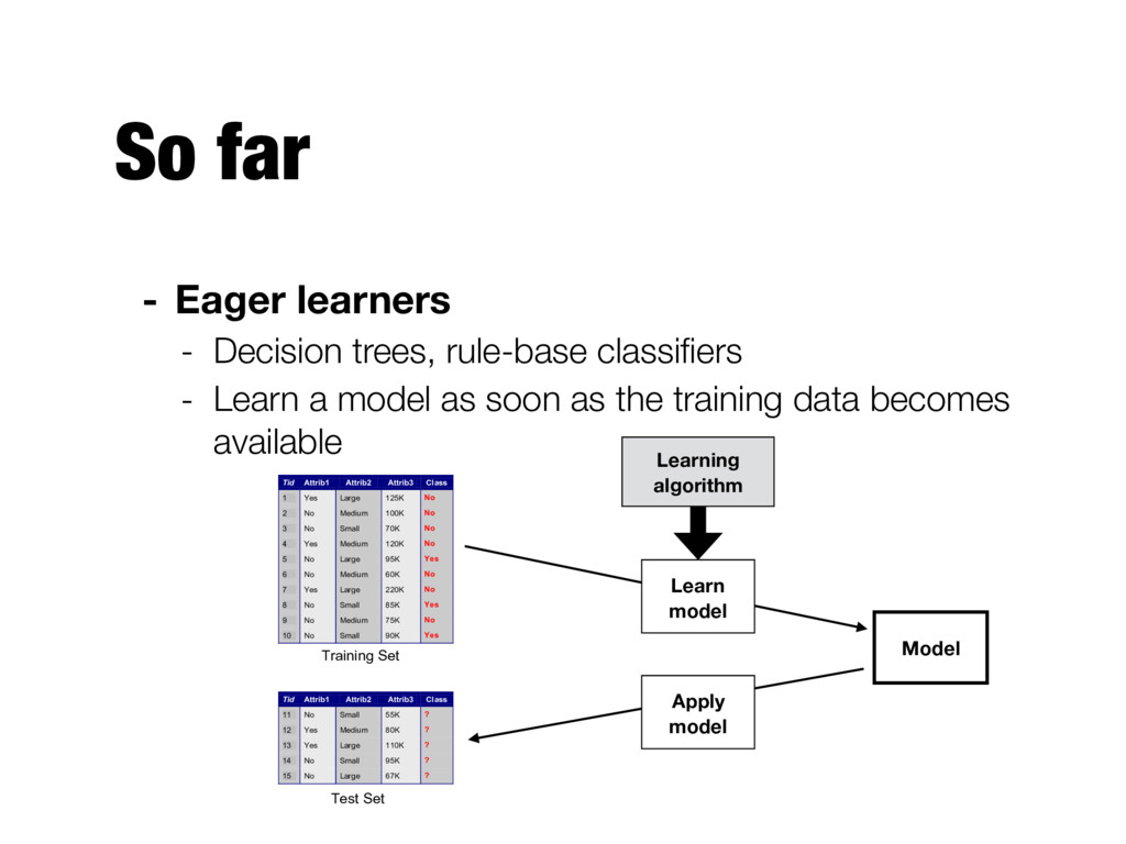
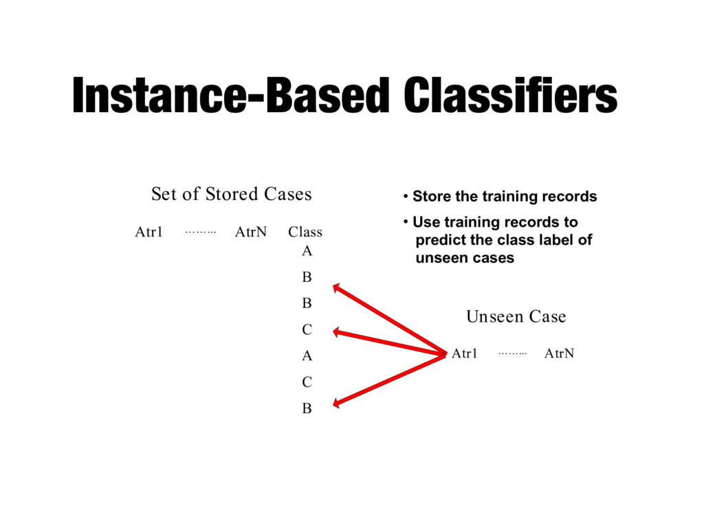
- Learn a model as soon as the training data becomes available Apply Model Induction Deduction Learn Model Model Tid Attrib1 Attrib2 Attrib3 Class 1 Yes Large 125K No 2 No Medium 100K No 3 No Small 70K No 4 Yes Medium 120K No 5 No Large 95K Yes 6 No Medium 60K No 7 Yes Large 220K No 8 No Small 85K Yes 9 No Medium 75K No 10 No Small 90K Yes 10 Tid Attrib1 Attrib2 Attrib3 Class 11 No Small 55K ? 12 Yes Medium 80K ? 13 Yes Large 110K ? 14 No Small 95K ? 15 No Large 67K ? 10 Test Set Learning algorithm Training Set Model Learning algorithm Learn model Apply model
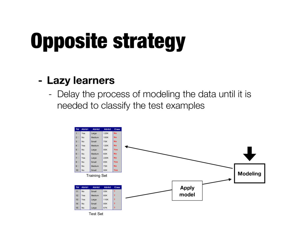
modeling the data until it is needed to classify the test examples Apply Model Induction Deduction Learn Model Model Tid Attrib1 Attrib2 Attrib3 Class 1 Yes Large 125K No 2 No Medium 100K No 3 No Small 70K No 4 Yes Medium 120K No 5 No Large 95K Yes 6 No Medium 60K No 7 Yes Large 220K No 8 No Small 85K Yes 9 No Medium 75K No 10 No Small 90K Yes 10 Tid Attrib1 Attrib2 Attrib3 Class 11 No Small 55K ? 12 Yes Medium 80K ? 13 Yes Large 110K ? 14 No Small 95K ? 15 No Large 67K ? 10 Test Set Learning algorithm Training Set Modeling Apply model
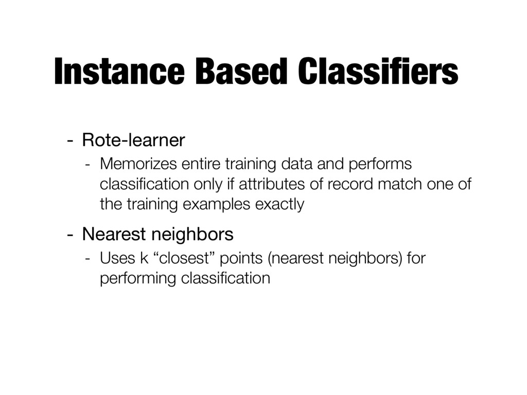
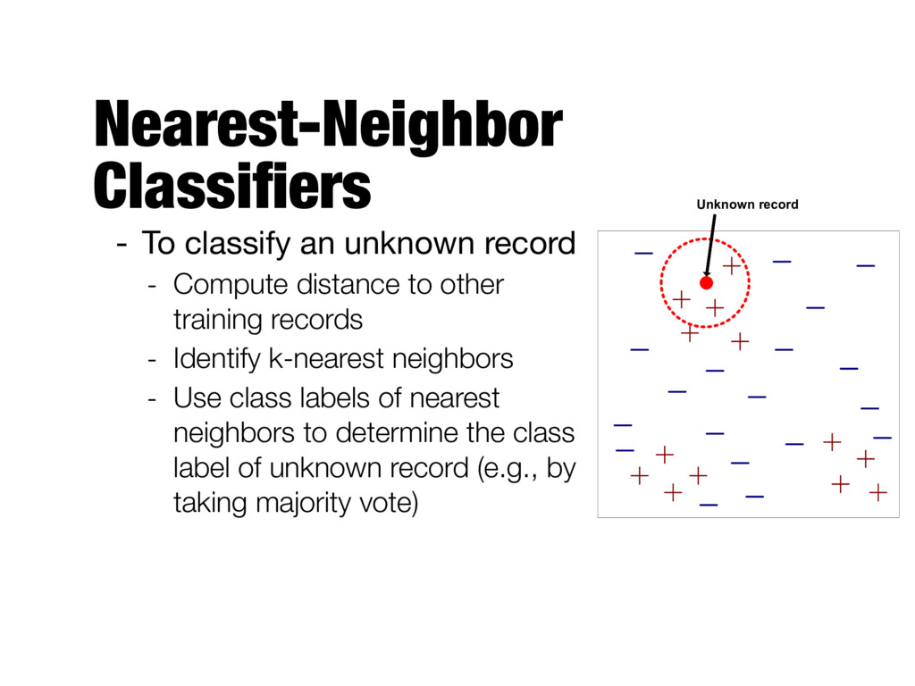
and performs classification only if attributes of record match one of the training examples exactly - Nearest neighbors - Uses k “closest” points (nearest neighbors) for performing classification
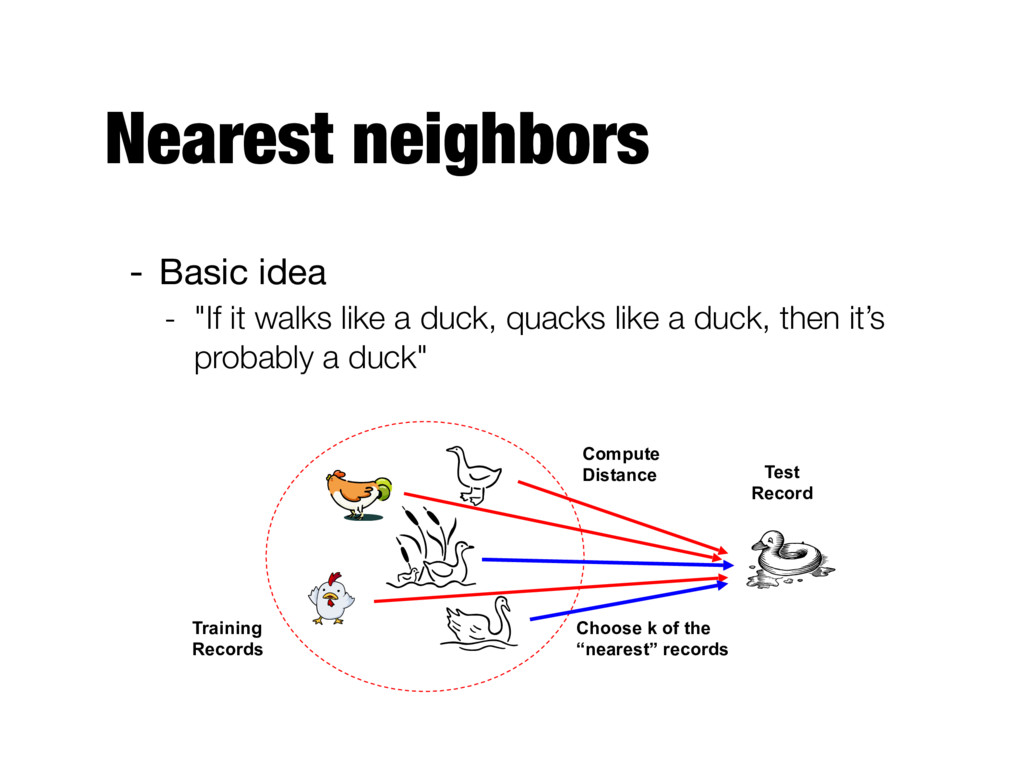
distance to other training records - Identify k-nearest neighbors - Use class labels of nearest neighbors to determine the class label of unknown record (e.g., by taking majority vote) Unknown record
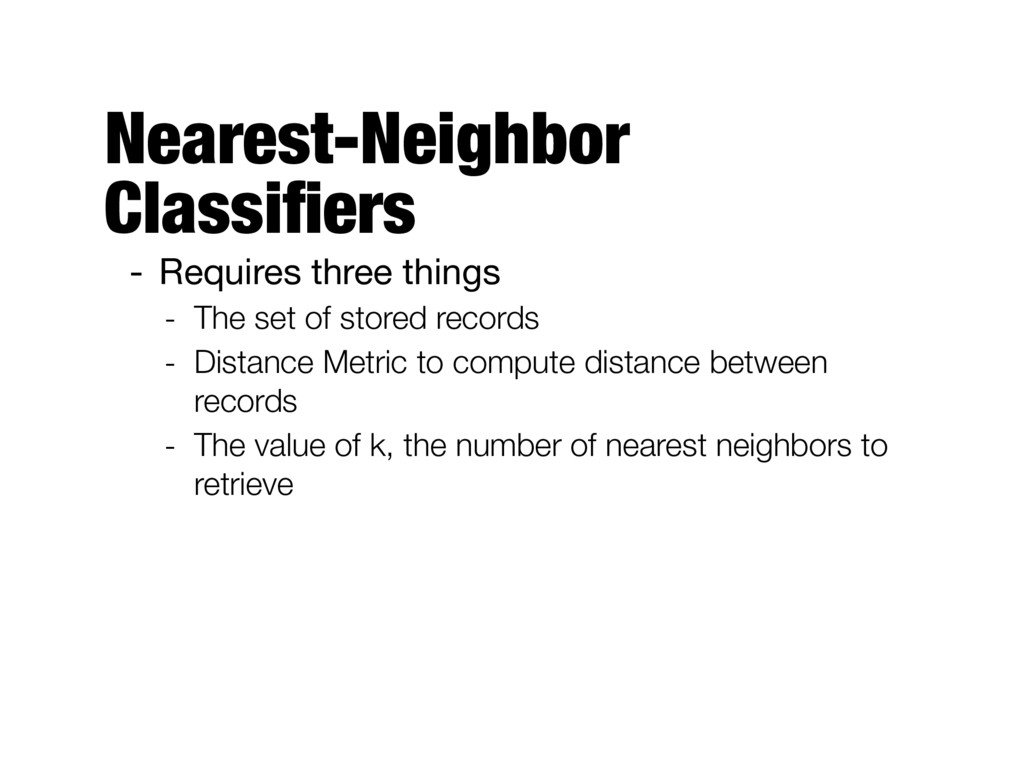
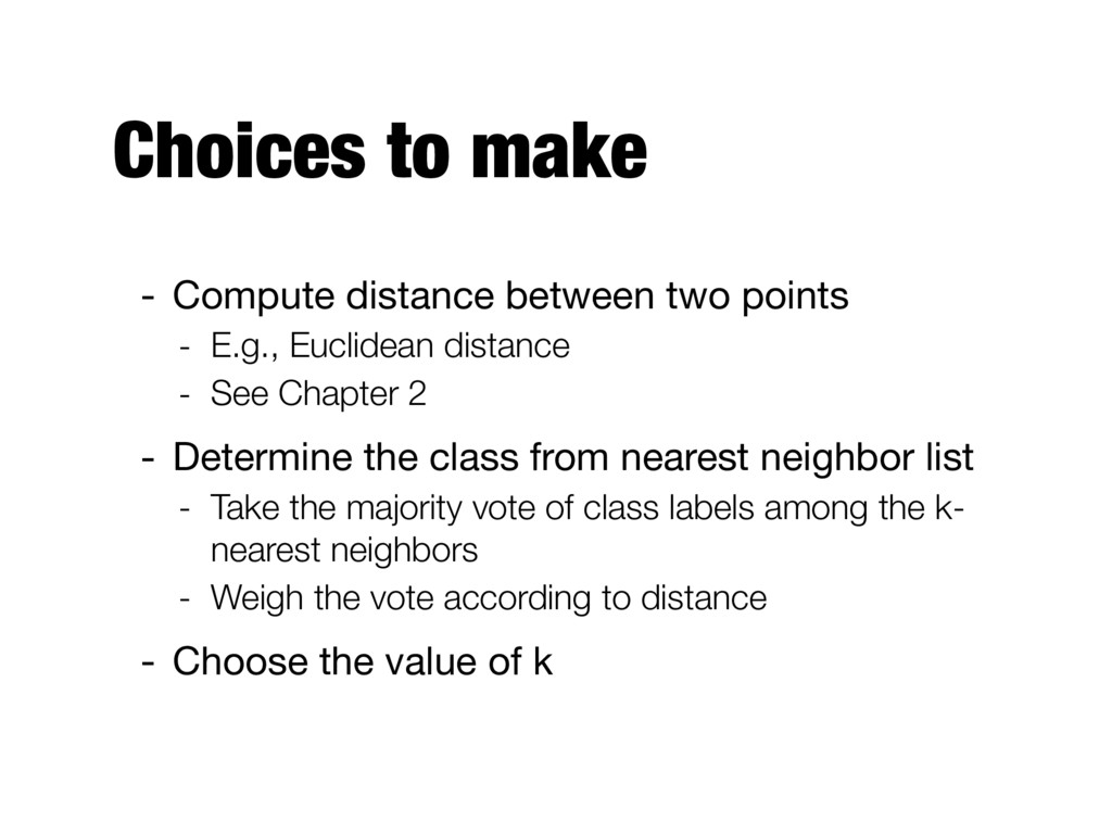
E.g., Euclidean distance - See Chapter 2 - Determine the class from nearest neighbor list - Take the majority vote of class labels among the k- nearest neighbors - Weigh the vote according to distance - Choose the value of k
learning - Use specific training instances to make predictions without having to maintain an abstraction (model) derived from data - Because there is no model building, classifying a test example can be quite expensive - Nearest-neighbors make their predictions based on local information - Susceptible to noise
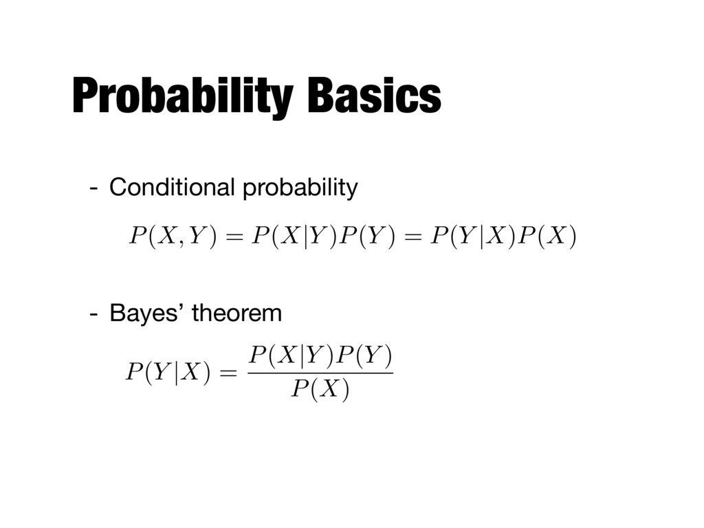
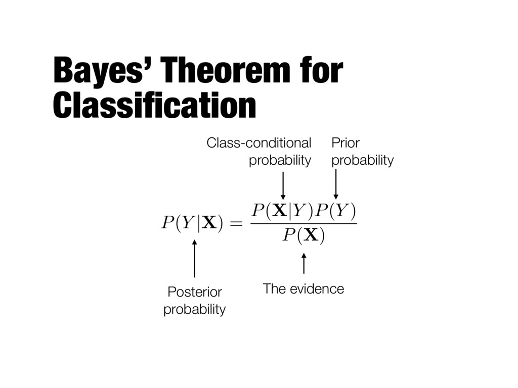
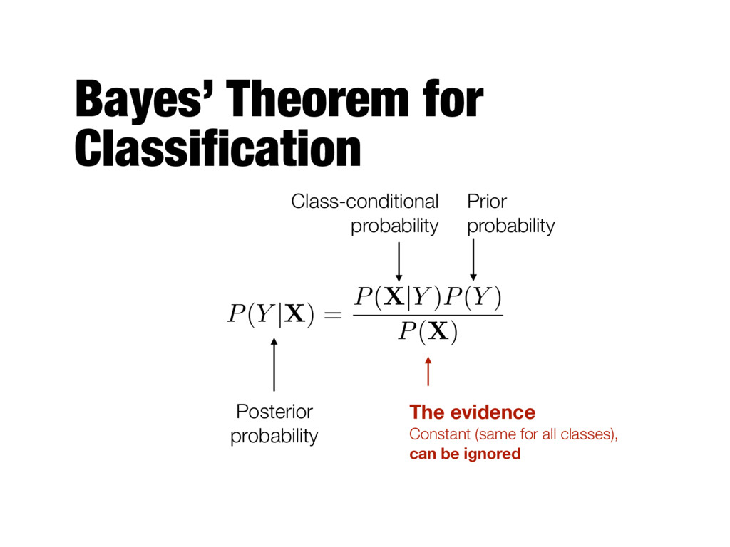
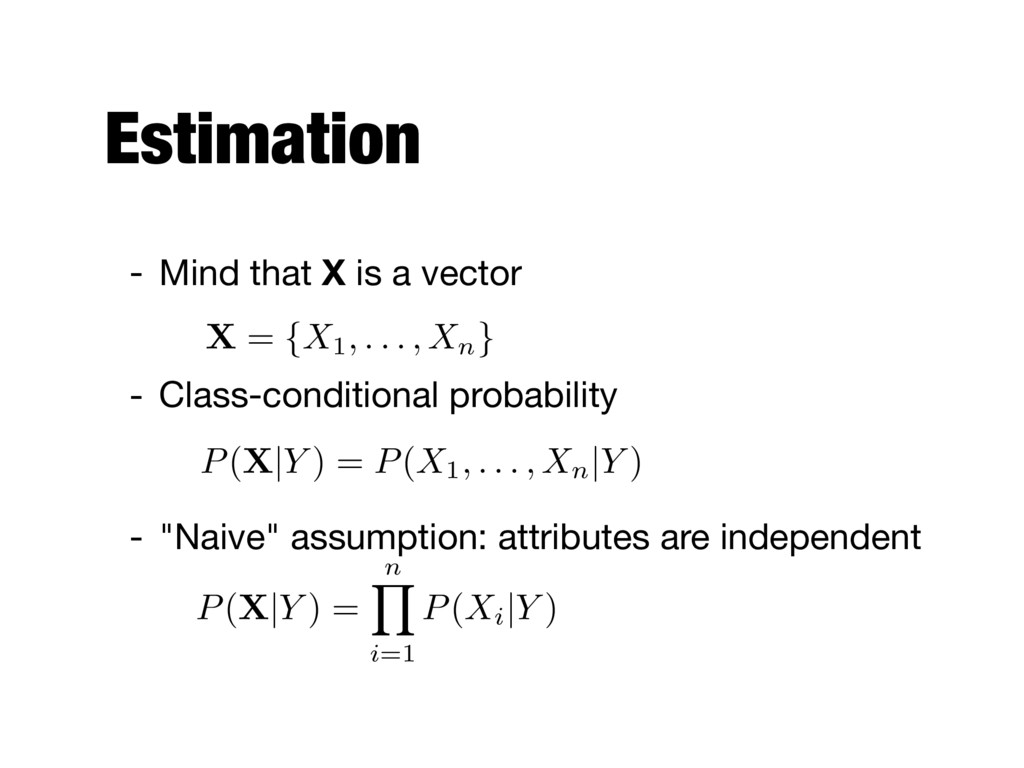
attribute set and the class variable is non-deterministic - The label of the test record cannot be predicted with certainty even if it was seen previously during training - A probabilistic framework for solving classification problems - Treat X and Y as random variables and capture their relationship probabilistically using P(Y|X)
Team A won 65% team B won 35% of the time - Among the games Team A won, 30% when game hosted by B - Among the games Team B won, 75% when B played home - Which team is more likely to win if the game is hosted by Team B?
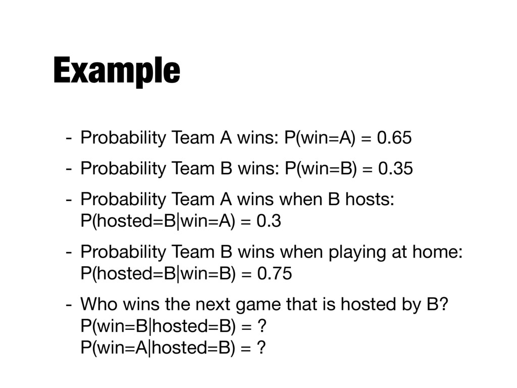
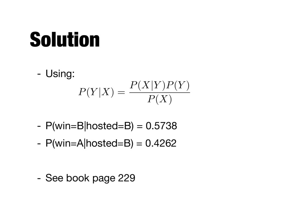
Probability Team B wins: P(win=B) = 0.35 - Probability Team A wins when B hosts: P(hosted=B|win=A) = 0.3 - Probability Team B wins when playing at home: P(hosted=B|win=B) = 0.75 - Who wins the next game that is hosted by B? P(win=B|hosted=B) = ? P(win=A|hosted=B) = ?
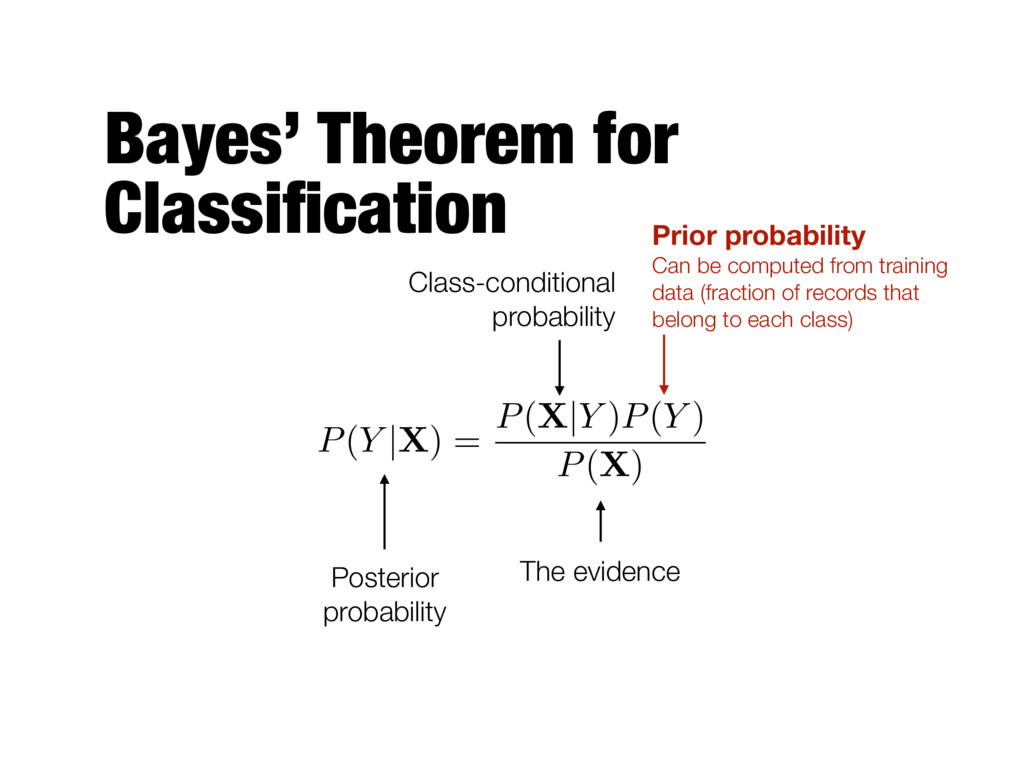
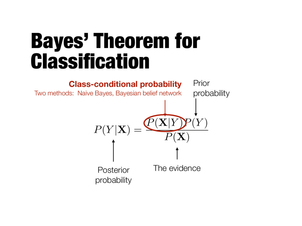
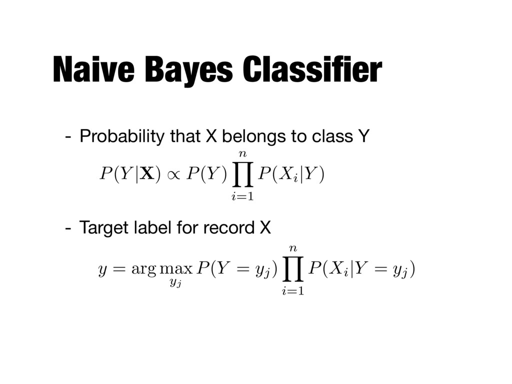
)P(Y ) P(X) The evidence Class-conditional probability Prior probability Can be computed from training data (fraction of records that belong to each class)
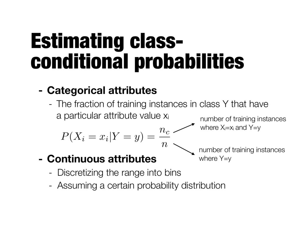
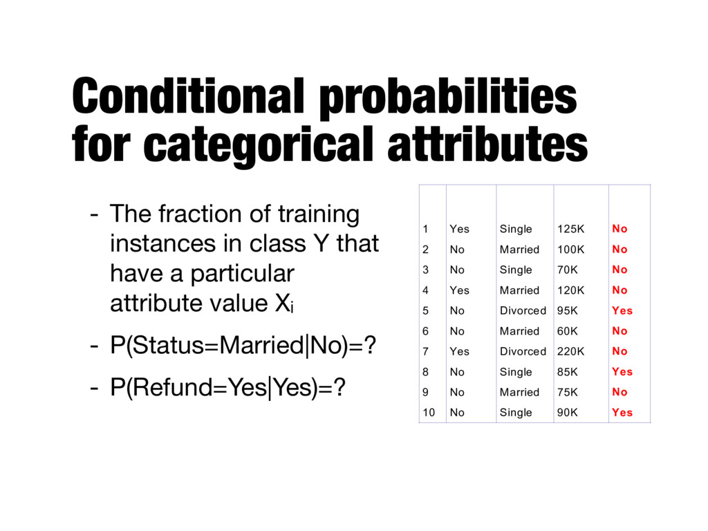
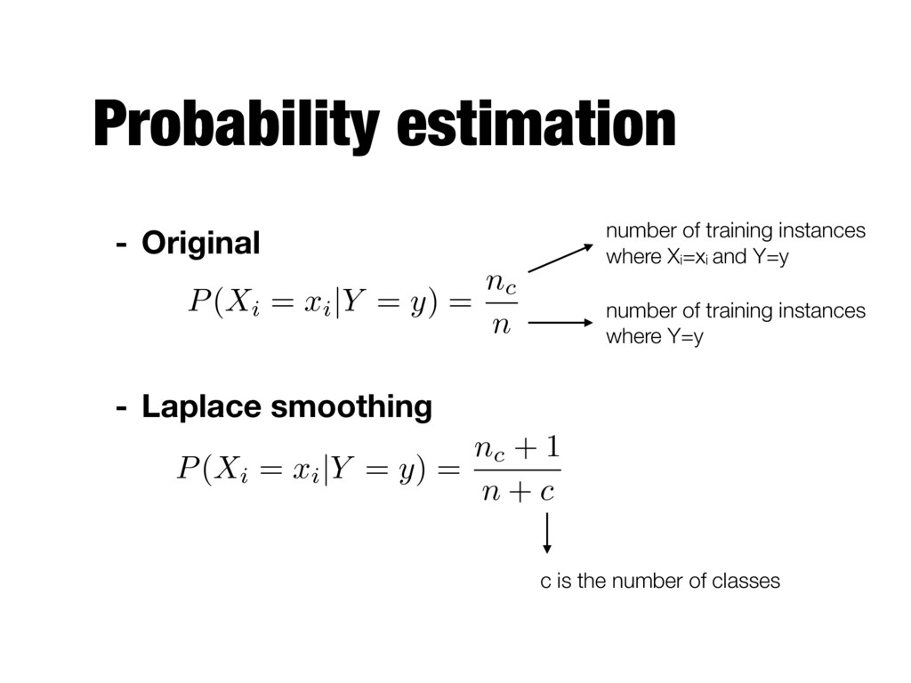
of training instances in class Y that have a particular attribute value xi - Continuous attributes - Discretizing the range into bins - Assuming a certain probability distribution number of training instances where Xi=xi and Y=y number of training instances where Y=y P ( Xi = xi | Y = y ) = nc n
instances in class Y that have a particular attribute value Xi - P(Status=Married|No)=? - P(Refund=Yes|Yes)=? Tid Refund Marital Status Taxable Income Evade 1 Yes Single 125K No 2 No Married 100K No 3 No Single 70K No 4 Yes Married 120K No 5 No Divorced 95K Yes 6 No Married 60K No 7 Yes Divorced 220K No 8 No Single 85K Yes 9 No Married 75K No 10 No Single 90K Yes 10 categorical categorical continuous class
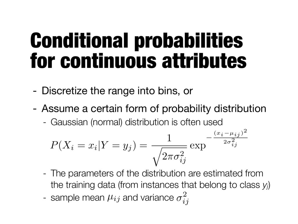
bins, or - Assume a certain form of probability distribution - Gaussian (normal) distribution is often used - The parameters of the distribution are estimated from the training data (from instances that belong to class yj) - sample mean and variance P(Xi = xi | Y = yj) = 1 q 2⇡ 2 ij exp ( xi µij )2 2 2 ij 2 ij µij
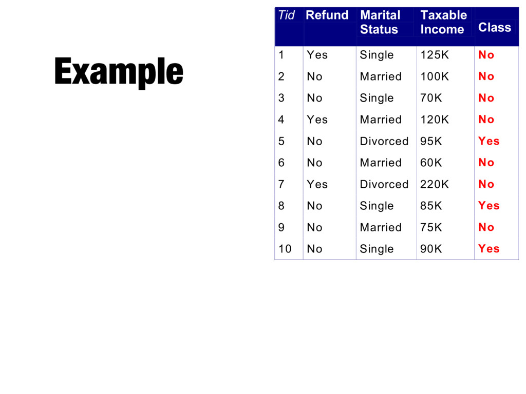
Single 125K No 2 No Married 100K No 3 No Single 70K No 4 Yes Married 120K No 5 No Divorced 95K Yes 6 No Married 60K No 7 Yes Divorced 220K No 8 No Single 85K Yes 9 No Married 75K No 10 No Single 90K Yes 10 Tid Refund Marital Status Taxable Income Class 1 Yes Single 125K No 2 No Married 100K No 3 No Single 70K No 4 Yes Married 120K No 5 No Divorced 95K Yes 6 No Married 60K No 7 Yes Divorced 220K No 8 No Single 85K Yes 9 No Married 75K No 10 No Single 90K Yes 10
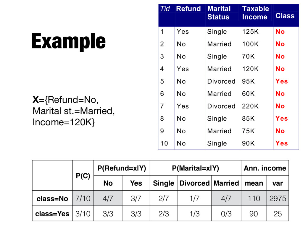
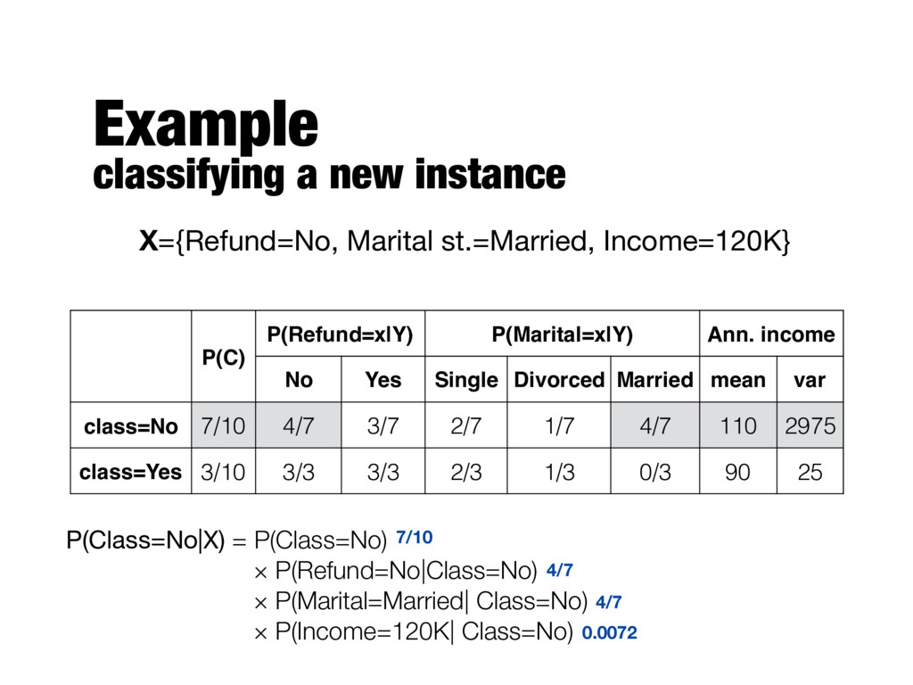
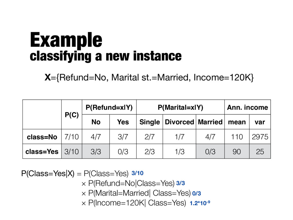
Single 125K No 2 No Married 100K No 3 No Single 70K No 4 Yes Married 120K No 5 No Divorced 95K Yes 6 No Married 60K No 7 Yes Divorced 220K No 8 No Single 85K Yes 9 No Married 75K No 10 No Single 90K Yes 10 Tid Refund Marital Status Taxable Income Class 1 Yes Single 125K No 2 No Married 100K No 3 No Single 70K No 4 Yes Married 120K No 5 No Divorced 95K Yes 6 No Married 60K No 7 Yes Divorced 220K No 8 No Single 85K Yes 9 No Married 75K No 10 No Single 90K Yes 10 X={Refund=No, Marital st.=Married, Income=120K} P(C) P(Refund=x|Y) P(Marital=x|Y) Ann. income No Yes Single Divorced Married mean var class=No 7/10 4/7 3/7 2/7 1/7 4/7 110 2975 class=Yes 3/10 3/3 3/3 2/3 1/3 0/3 90 25
instances where Xi=xi and Y=y number of training instances where Y=y P ( Xi = xi | Y = y ) = nc n P ( Xi = xi | Y = y ) = nc + 1 n + c c is the number of classes
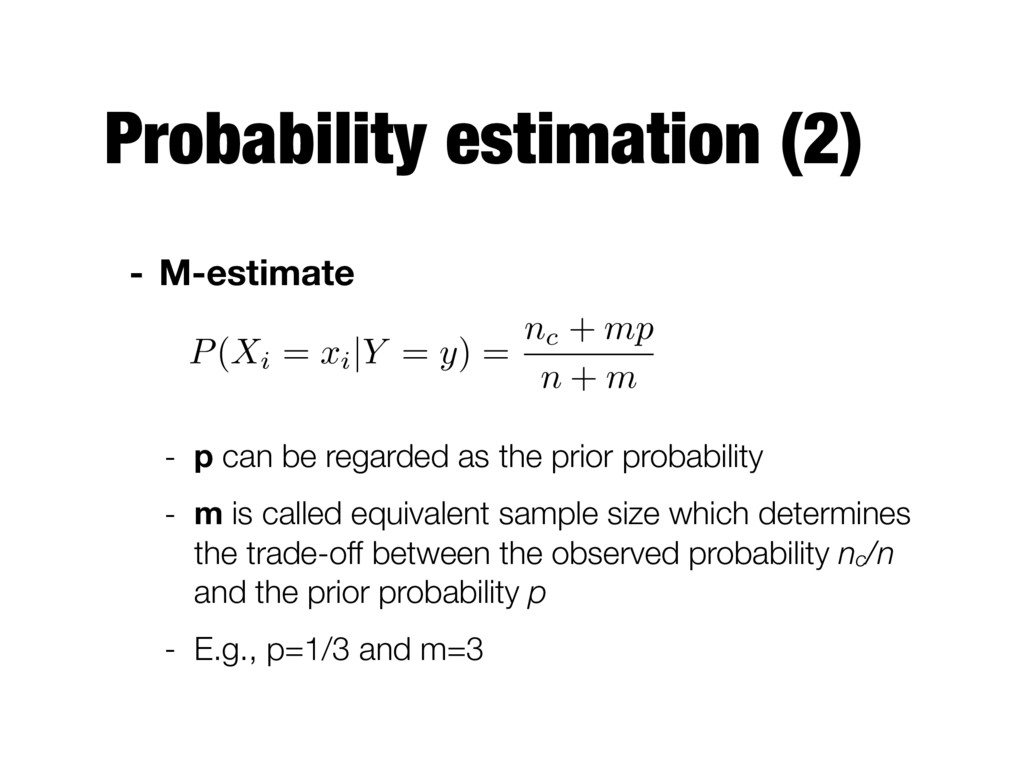
as the prior probability - m is called equivalent sample size which determines the trade-off between the observed probability nc/n and the prior probability p - E.g., p=1/3 and m=3 P ( Xi = xi | Y = y ) = nc + mp n + m
values by ignoring the instance during probability estimate calculations - Robust to irrelevant attributes - Independence assumption may not hold for some attributes
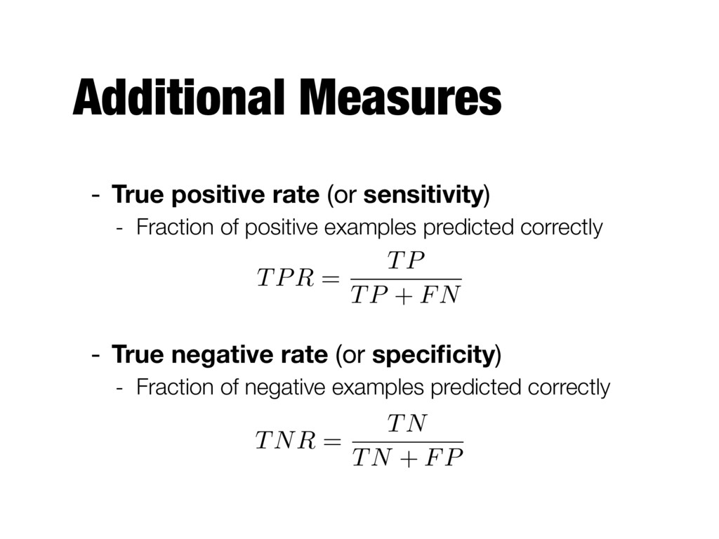
are quite common in real-world applications - E.g., credit card fraud detection - Correct classification of the rare class has often greater value than a correct classification of the majority class - The accuracy measure is not well suited for imbalanced data sets - We need alternative measures
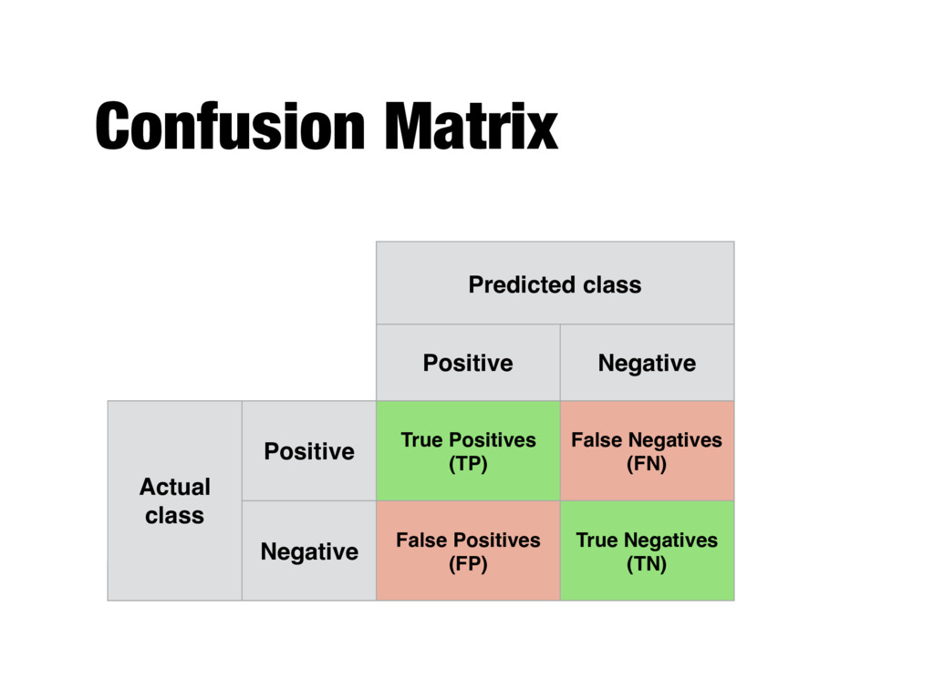
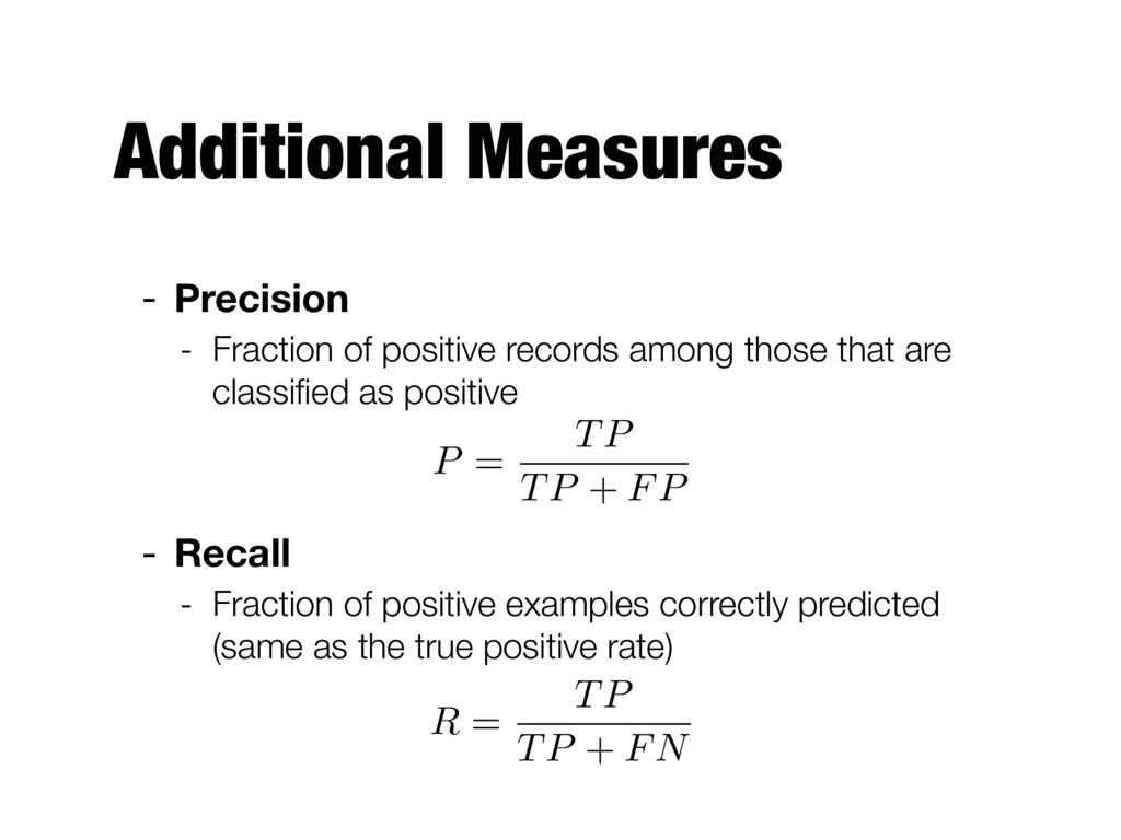
those that are classified as positive - Recall - Fraction of positive examples correctly predicted (same as the true positive rate) P = TP TP + FP R = TP TP + FN
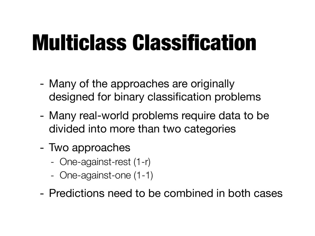
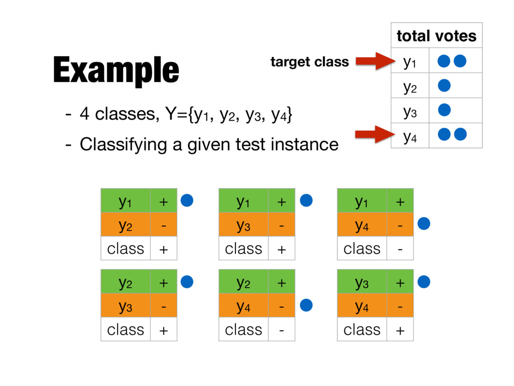
for binary classification problems - Many real-world problems require data to be divided into more than two categories - Two approaches - One-against-rest (1-r) - One-against-one (1-1) - Predictions need to be combined in both cases
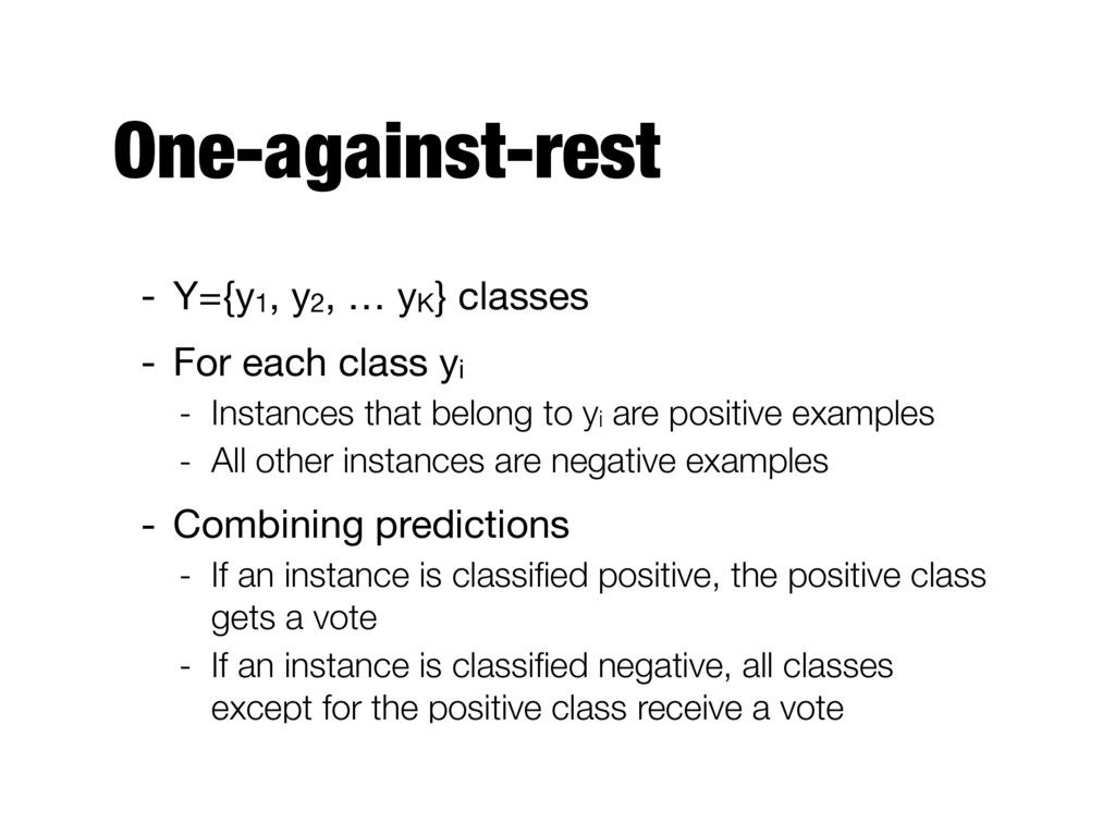
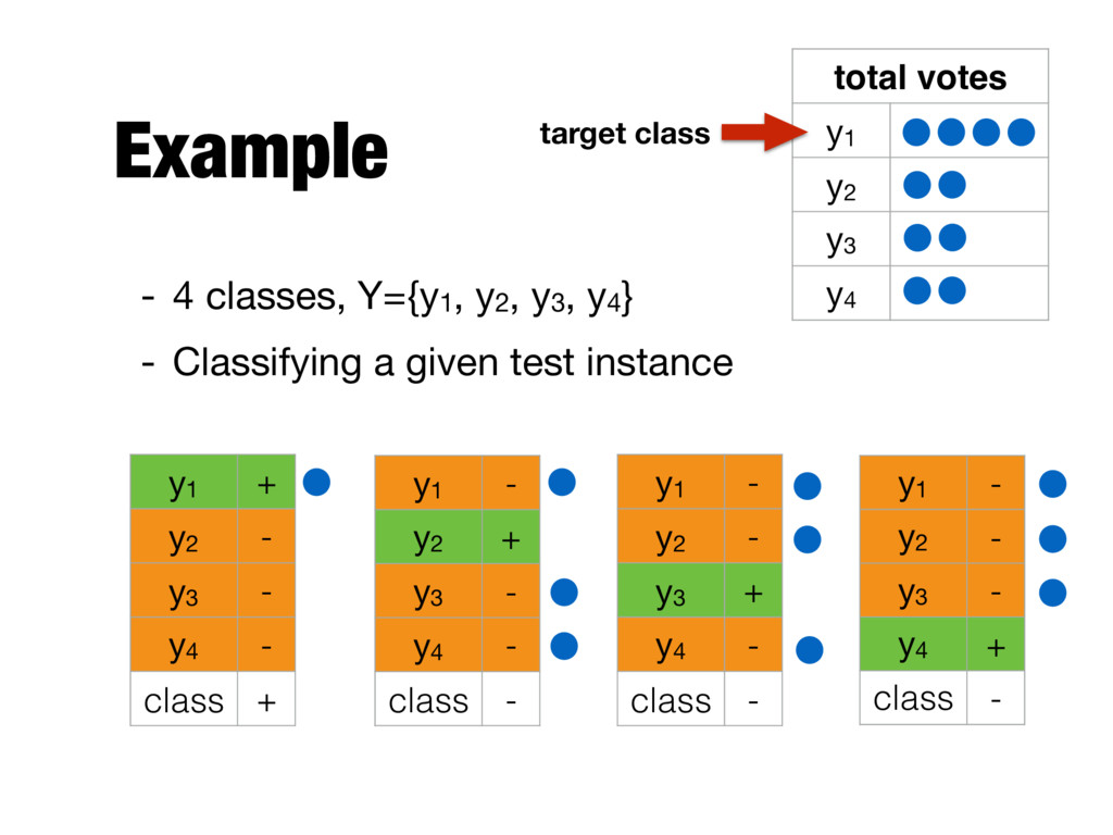
class yi - Instances that belong to yi are positive examples - All other instances are negative examples - Combining predictions - If an instance is classified positive, the positive class gets a vote - If an instance is classified negative, all classes except for the positive class receive a vote
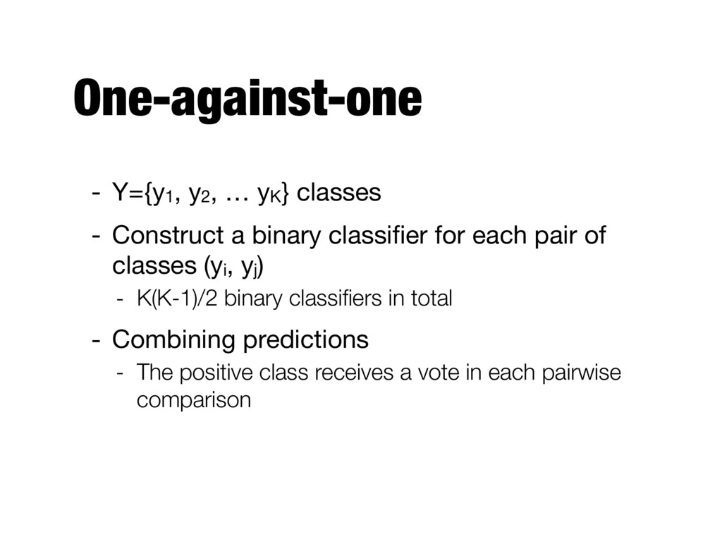
binary classifier for each pair of classes (yi, yj) - K(K-1)/2 binary classifiers in total - Combining predictions - The positive class receives a vote in each pairwise comparison
a given test instance y1 + y2 - class + y1 + y3 - class + y1 + y4 - class - y2 + y3 - class + y2 + y4 - class - y3 + y4 - class + total votes y1 y2 y3 y4 target class