Information Retrieval and Text Mining 2020 - Neural IR

University of Stavanger, DAT640, 2020 fall

Transcript

1. Neural IR [DAT640] Informa on Retrieval and Text Mining Trond Linjordet University of Stavanger October 12, 2020 CC BY 4.0
2. Outline (Neural IR) • Neural Networks • Word Embeddings - Word2Vec • Neural IR Models 2 / 35
3. Neural Networks 3 / 35
4. Neural networks: The Perceptron • The perceptron illustrates the idea of an artificial neuron, or activation unit. z = b + j wj × xj y = factivation(z) ˙ = 0 if z > 0 1 if z ≤ 0 Figure: The perceptron. 4 / 35
5. Neural networks: Mul layer perceptron • Continuous non-linear functions with defined derivatives, e.g. the sigmoid logistic function: factivation(z) = σ(z) = 1 1 + e−z Figure: One example of a multilayer perceptron. 5 / 35
6. Neural networks: Mul layer perceptron • Example MLP from previous slide, feedforward as equation: y = σ(W(3) h(2) + b(3)) = σ(W(3) σ(W(2) h(1) + b(2)) + b(3)) = σ(W(3) σ(W(2) σ(W(1) x + b(1)) + b(2)) + b(3)) • Loss function: J(θ) ∝ ||y − f(x; θ)|| • Gradient descent to minimize loss: θnew ← θold − α∇θold J(θold) • Backpropagation, the chain rule, and vanishing gradients: ∂ ∂w(L) j J(θ) = ∂z(L) ∂w(L) j ∂h(L) ∂z(L) ∂J(θ) ∂h(L) 6 / 35
7. Word Embeddings - Word2Vec 7 / 35
8. Word embeddings - background • Vector space models (e.g. TF-IDF) Figure: Vector space model. Illustration is taken from (Zhai&Massung, 2016)[Fig. 6.2] 8 / 35
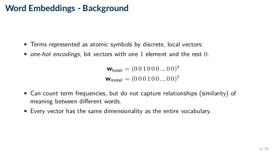
9. Word Embeddings - Background • Terms represented as atomic symbols by discrete, local vectors: • one-hot encodings, bit vectors with one 1 element and the rest 0. whotel = (0 0 1 0 0 0 ... 0 0) wmotel = (0 0 0 1 0 0 ... 0 0) • Can count term frequencies, but do not capture relationships (similarity) of meaning between different words. • Every vector has the same dimensionality as the entire vocabulary. 9 / 35
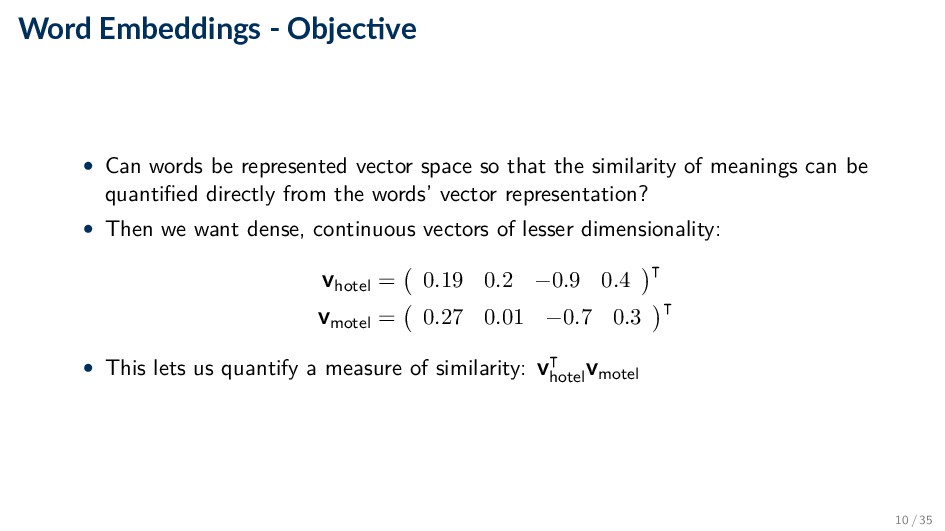
10. Word Embeddings - Objec ve • Can words be represented vector space so that the similarity of meanings can be quantified directly from the words’ vector representation? • Then we want dense, continuous vectors of lesser dimensionality: vhotel = 0.19 0.2 −0.9 0.4 vmotel = 0.27 0.01 −0.7 0.3 • This lets us quantify a measure of similarity: v hotel vmotel 10 / 35
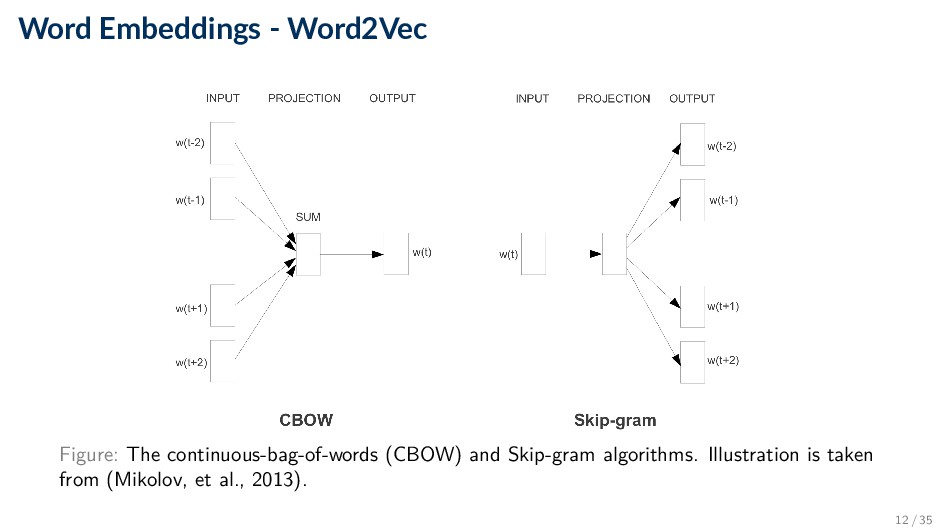
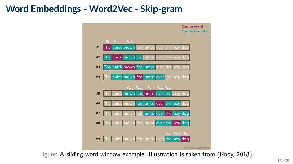
11. Word Embeddings - Word2Vec • Distributional hypothesis: “You shall know a word by the company it keeps.” (Firth, J. R., 1957) • Word2Vec (Mikolov, 2013) • Represent words based on the contexts in which they occur. • CBOW: Predict target word wt based on context words wt−j, wt+j within some context window C around wt . • Skip-gram: Predict context words wt−j, wt+j within some context window C with radius m around wt, based on wt. ◦ We will focus on this algorithm. 11 / 35
12. Word Embeddings - Word2Vec Figure: The continuous-bag-of-words (CBOW) and Skip-gram algorithms. Illustration is taken from (Mikolov, et al., 2013). 12 / 35
13. Word Embeddings - Word2Vec - Skip-gram Figure: A sliding word window example. Illustration is taken from (Rooy, 2018). 13 / 35
14. Word Embeddings - Word2Vec - Skip-gram • Maximize the probability of true context words wt−m, wt−m+1, ..., wt−1, wt+1, ..., wt+m−1, wt+m for each target word wt: J (θ) = T t=1 −m ≤ j ≤ m j = 0 P(wt+j|wt; θ) • Negative Log Likelihood: J(θ) = − 1 T T t=1 −m ≤ j ≤ m j = 0 log P(wt+j|wt; θ) 14 / 35
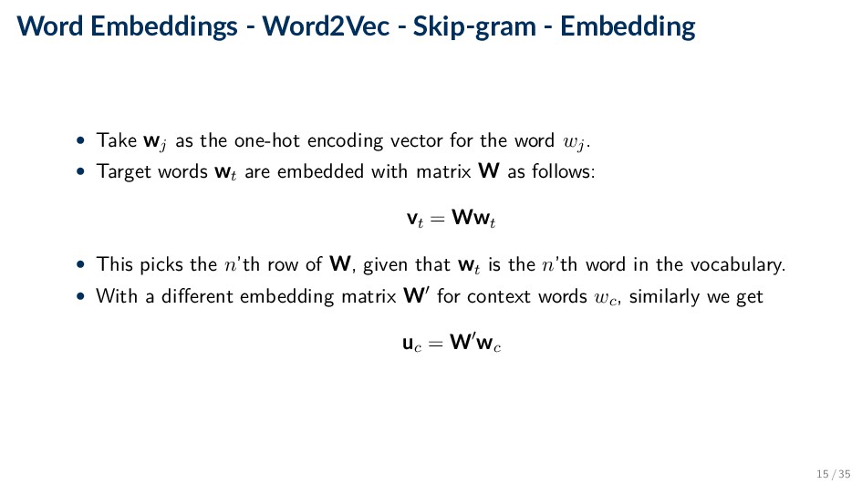
15. Word Embeddings - Word2Vec - Skip-gram - Embedding • Take wj as the one-hot encoding vector for the word wj. • Target words wt are embedded with matrix W as follows: vt = Wwt • This picks the n’th row of W, given that wt is the n’th word in the vocabulary. • With a different embedding matrix W for context words wc, similarly we get uc = W wc 15 / 35
16. Word Embeddings - Word2Vec - Skip-gram - Visualiza on Figure: Forward pass of Skip-gram. Illustration is taken from (L. Weng, 2017). 16 / 35
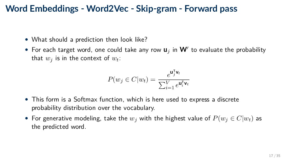
17. Word Embeddings - Word2Vec - Skip-gram - Forward pass • What should a prediction then look like? • For each target word, one could take any row uj in W to evaluate the probability that wj is in the context of wt: P(wj ∈ C|wt) = eu j vt V i=1 eu i vt • This form is a Softmax function, which is here used to express a discrete probability distribution over the vocabulary. • For generative modeling, take the wj with the highest value of P(wj ∈ C|wt) as the predicted word. 17 / 35
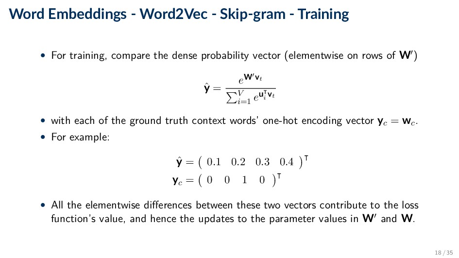
18. Word Embeddings - Word2Vec - Skip-gram - Training • For training, compare the dense probability vector (elementwise on rows of W ) ˆ y = eW vt V i=1 eu i vt • with each of the ground truth context words’ one-hot encoding vector yc = wc. • For example: ˆ y = 0.1 0.2 0.3 0.4 yc = 0 0 1 0 • All the elementwise differences between these two vectors contribute to the loss function’s value, and hence the updates to the parameter values in W and W. 18 / 35
19. Word Embeddings - Word2Vec - Skip-gram - Training • For training, compare the dense probability vector (elementwise on rows of W ) ˆ y = eW vt V i=1 eu i vt with each of the ground truth context words’ one-hot encoding vector yc = wc. • For example: ˆ y = 0.1 0.2 0.3 0.4 yc = 0 0 1 0 • All the elementwise differences between these two vectors contribute to the loss function’s value, and hence the updates to the parameter values in W and W. 19 / 35
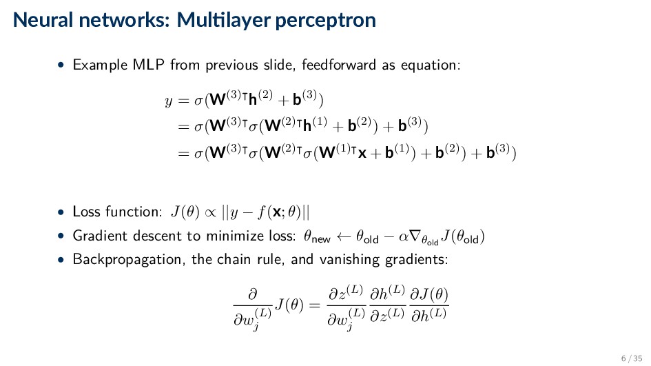
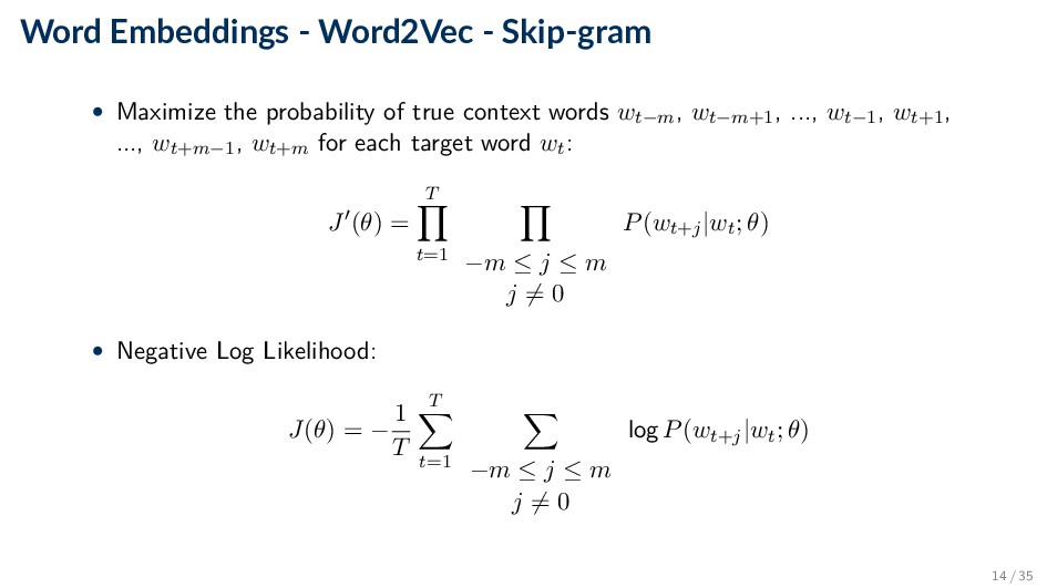
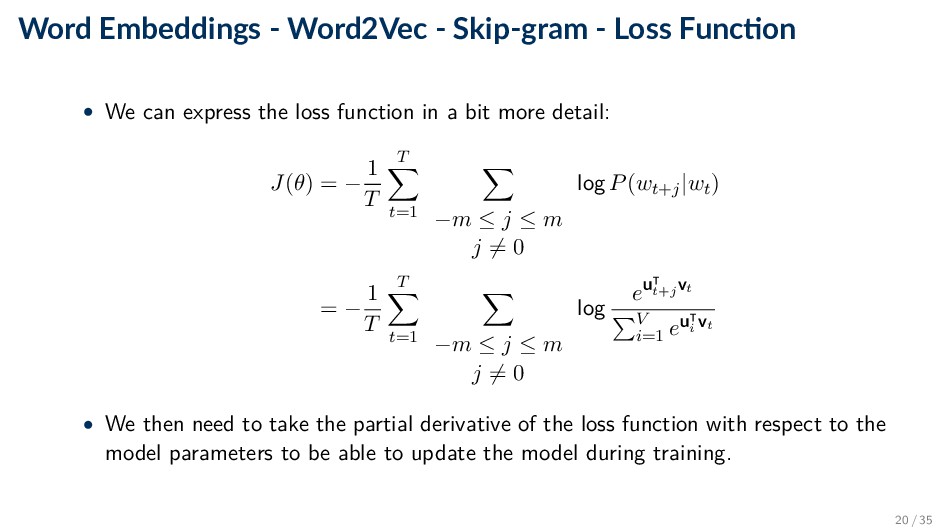
20. Word Embeddings - Word2Vec - Skip-gram - Loss Func on • We can express the loss function in a bit more detail: J(θ) = − 1 T T t=1 −m ≤ j ≤ m j = 0 log P(wt+j|wt) = − 1 T T t=1 −m ≤ j ≤ m j = 0 log eu t+j vt V i=1 eu i vt • We then need to take the partial derivative of the loss function with respect to the model parameters to be able to update the model during training. 20 / 35
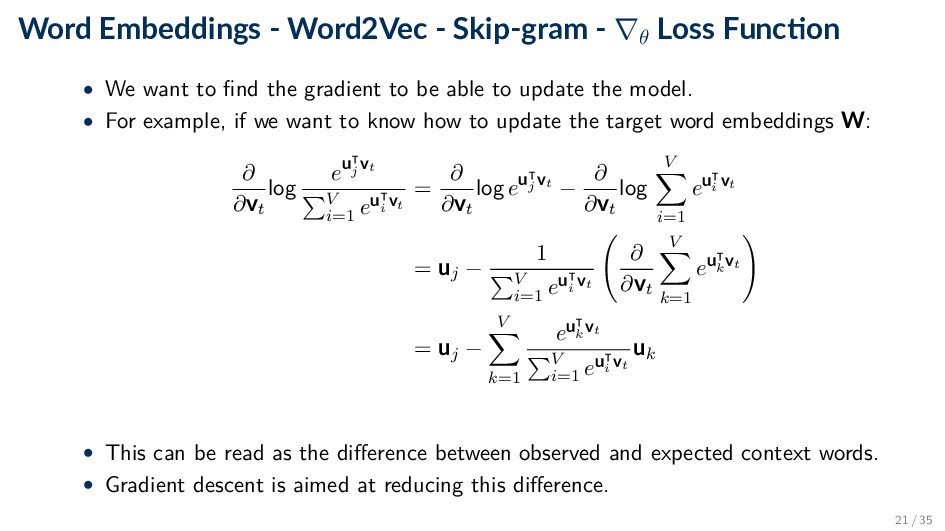
21. Word Embeddings - Word2Vec - Skip-gram - ∇θ Loss Func on • We want to find the gradient to be able to update the model. • For example, if we want to know how to update the target word embeddings W: ∂ ∂vt log eu j vt V i=1 eu i vt = ∂ ∂vt log eu j vt − ∂ ∂vt log V i=1 eu i vt = uj − 1 V i=1 eu i vt ∂ ∂vt V k=1 eu k vt = uj − V k=1 eu k vt V i=1 eu i vt uk • This can be read as the difference between observed and expected context words. • Gradient descent is aimed at reducing this difference. 21 / 35
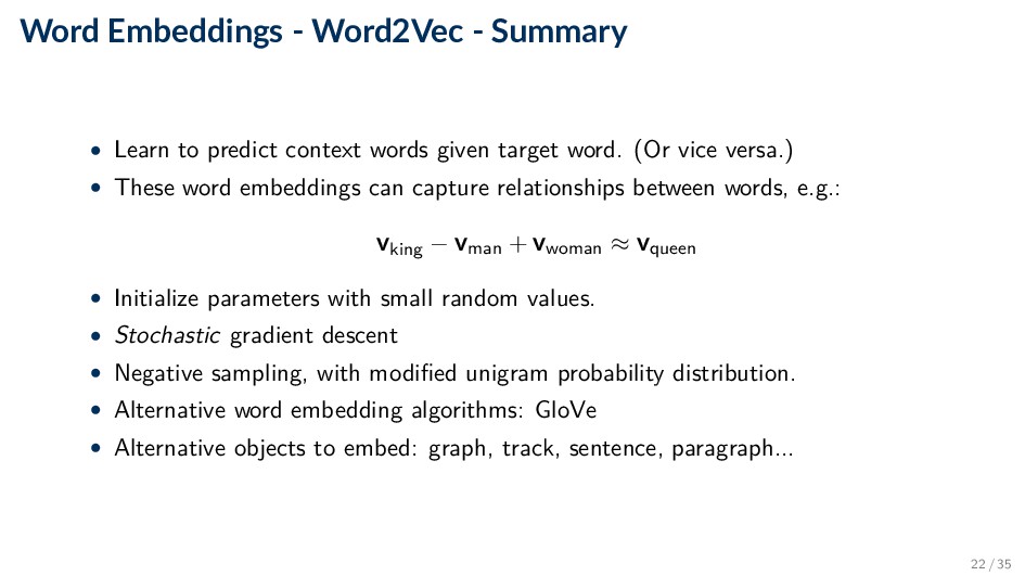
22. Word Embeddings - Word2Vec - Summary • Learn to predict context words given target word. (Or vice versa.) • These word embeddings can capture relationships between words, e.g.: vking − vman + vwoman ≈ vqueen • Initialize parameters with small random values. • Stochastic gradient descent • Negative sampling, with modified unigram probability distribution. • Alternative word embedding algorithms: GloVe • Alternative objects to embed: graph, track, sentence, paragraph... 22 / 35
23. Neural IR Models 23 / 35
24. Discussion • How could word embeddings trained using Word2Vec (or a similar) be used for determining the relevance of documents to queries? 24 / 35
25. Informa on Retrieval using Word Embeddings • Scoring with embeddings ◦ Relevance ∼ Similarity? ◦ Relevance ∼ Distance−1 ? How do these quantities relate? ◦ Use one or two embedding matrices? • Decisions: (Regression, classification) ×(Scoring, ranking). • Projecting multiword texts into embedding space: ◦ Centroid? ◦ Pairwise comparison of query and candidate document words? f(wq , wd ) • We will look at some early models of neural IR. 25 / 35
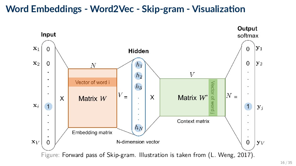
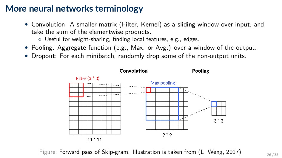
26. More neural networks terminology • Convolution: A smaller matrix (Filter, Kernel) as a sliding window over input, and take the sum of the elementwise products. ◦ Useful for weight-sharing, finding local features, e.g., edges. • Pooling: Aggregate function (e.g., Max. or Avg.) over a window of the output. • Dropout: For each minibatch, randomly drop some of the non-output units. Figure: Forward pass of Skip-gram. Illustration is taken from (L. Weng, 2017). 26 / 35
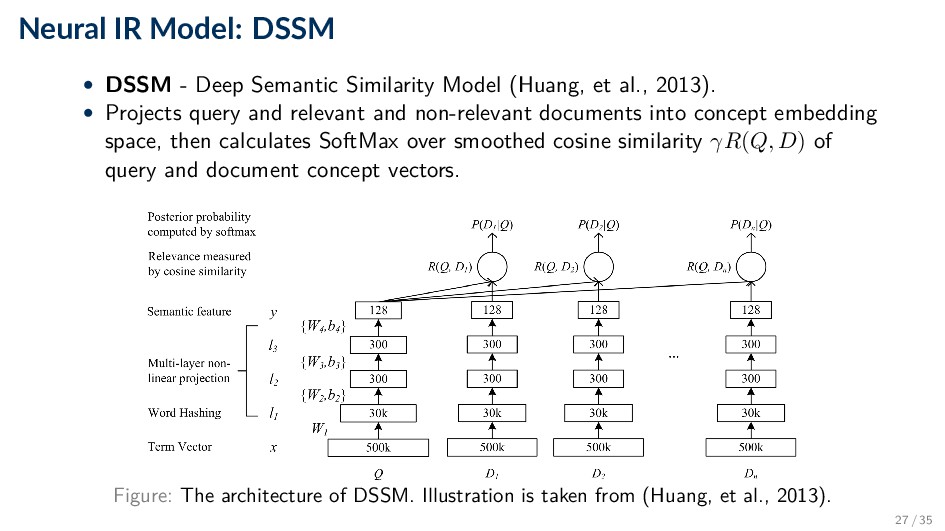
27. Neural IR Model: DSSM • DSSM - Deep Semantic Similarity Model (Huang, et al., 2013). • Projects query and relevant and non-relevant documents into concept embedding space, then calculates SoftMax over smoothed cosine similarity γR(Q, D) of query and document concept vectors. Figure: The architecture of DSSM. Illustration is taken from (Huang, et al., 2013). 27 / 35
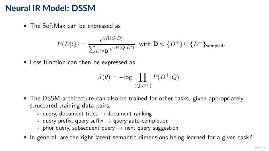
28. Neural IR Model: DSSM • The SoftMax can be expressed as P(D|Q) = eγR(Q,D) D ∈D eγR(Q,D ) , with D ≈ {D+} ∪ {D−}sampled. • Loss function can then be expressed as J(θ) = −log (Q,D+) P(D+|Q). • The DSSM architecture can also be trained for other tasks, given appropriately structured training data pairs: ◦ query, document titles → document ranking ◦ query prefix, query suffix → query auto-completion ◦ prior query, subsequent query → next query suggestion • In general, are the right latent semantic dimensions being learned for a given task? 28 / 35
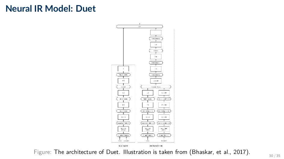
29. Neural IR Model: Duet • One strength of local representations over distributed representation is for very rare words in the vocabulary! • “Aardvark” may not occur often enough to get a very useful word embedding, but its one-hot encoding can still give an exact match. • Duet - Learning to Match Using Local and Distributed Representations of Text for Web Search (Bhaskar, et al., 2017). • This architecture trains two separate deep neural network submodels jointly, one on local representations and the other on distributed representations. • Both have submodels include convolution. f(Q, D) = fl(Q, D) + fd(Q, D) 29 / 35
30. Neural IR Model: Duet Figure: The architecture of Duet. Illustration is taken from (Bhaskar, et al., 2017). 30 / 35
31. Neural IR Model: NRM-F • NRM-F - Neural Ranking Models with Multiple Document Fields (Zamani, et al., 2017). Illustrations are taken from (Zamani, et al., 2017). Figure: High-level NRM-F architecture. Figure: Multi-field representation embedding. Figure: Instance-level representation learning. 31 / 35
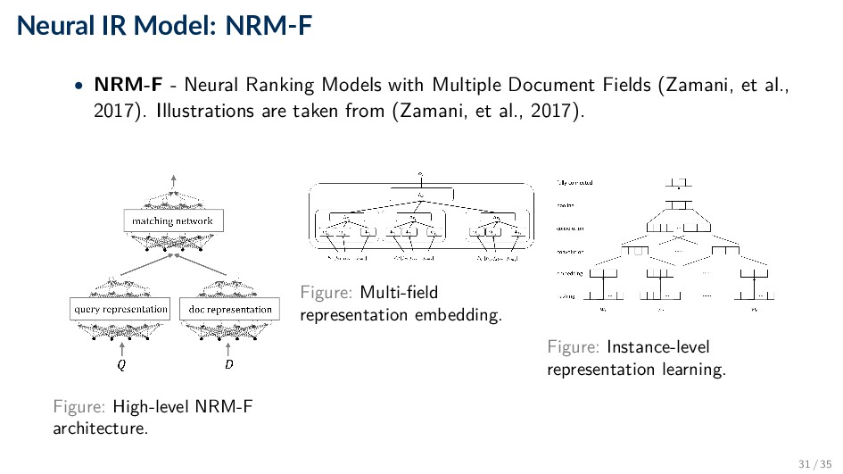
32. Neural IR Model: NRM-F • A specific query embedding is learned for each field in the documents, and a specific document embedding is learned for each field in the documents. • As these field-specific representations have the same dimensions, a Hadamard product for each field, qi,f ◦ dj,f is concatenated, with field-level dropout, and passed to the fully-connected matching network. 32 / 35
33. Conclusion • Neural methods can complement traditional IR methods. • A variety of patterns can be combined in different configurations. 33 / 35
34. References • Text Data Management and Analysis (Zhai&Massung), Chapters 6. • T. Mikolov, K. Chen, G. Corrado, and J. Dean. Efficient Estimation of Word Representations in Vector Space. In Proc. of ICLR, 2013. • YouTube: Chris Manning, Lecture 2: Word2Vec - Deep Learning for NLP, Stanford, 2017. • YouTube: Richard Socher, Lecture 3: GloVe - Deep Learning for NLP, Stanford, 2017. • Word2vec from Scratch with Python and NumPy, Nathan Rooy, March 22, 2018. ◦ https://nathanrooy.github.io/posts/2018-03-22/ word2vec-from-scratch-with-python-and-numpy • Learning Word Embedding, Lilian Weng, Oct 15, 2017. ◦ https://lilianweng.github.io/lil-log/2017/10/15/ learning-word-embedding.html 34 / 35
35. References (con nued) • YouTube: Bhaskar Mitra, Neural Models for Information Retrieval, Microsoft Research, 2018. • P.S. Huang, X. He, J. Gao, L. Deng, A. Acero, and L. Heck. Learning Deep Structured Semantic Models for Web Search using Clickthrough Data . In Proc. of CIKM, 2013. • B. Mitra, F. Diaz, and N. Craswell. Learning to Match Using Local and Distributed Representations of Text for Web Search. In Proc. of WWW, 2017. • H. Zamani, B. Mitra, X. Song, N. Craswell, and S. Tiwary. Neural Ranking Models with Multiple Document Fields. In Proc. of WSDM, 2017. 35 / 35