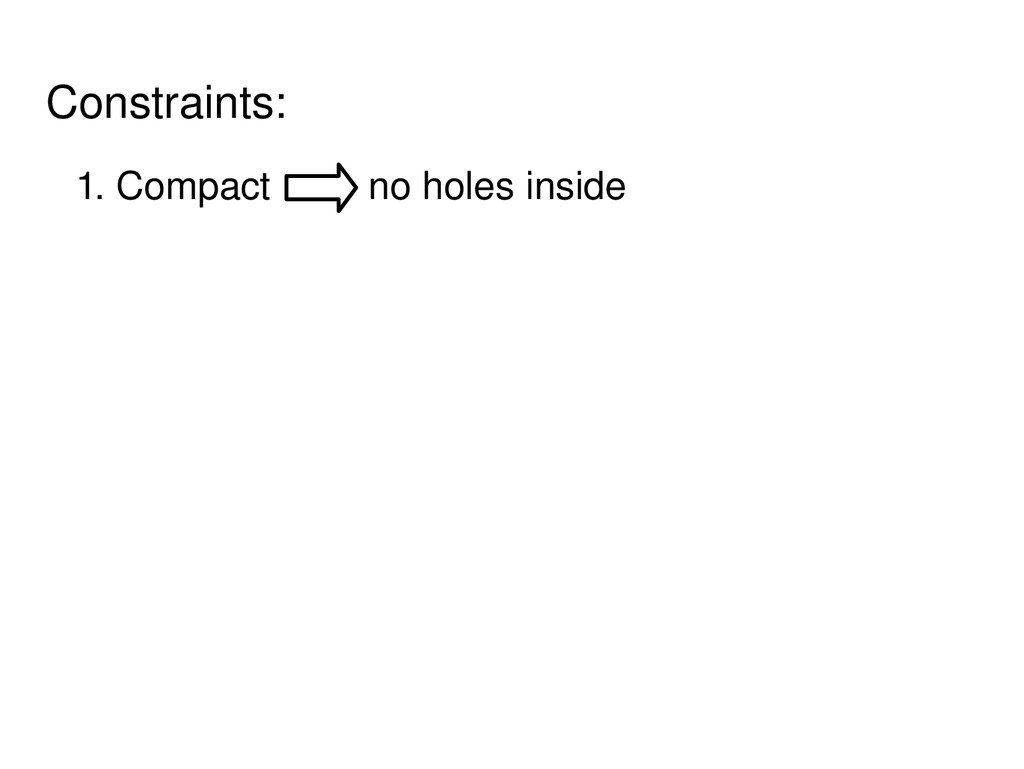
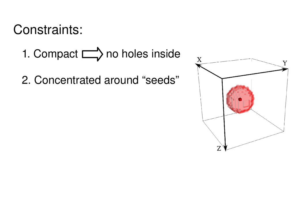
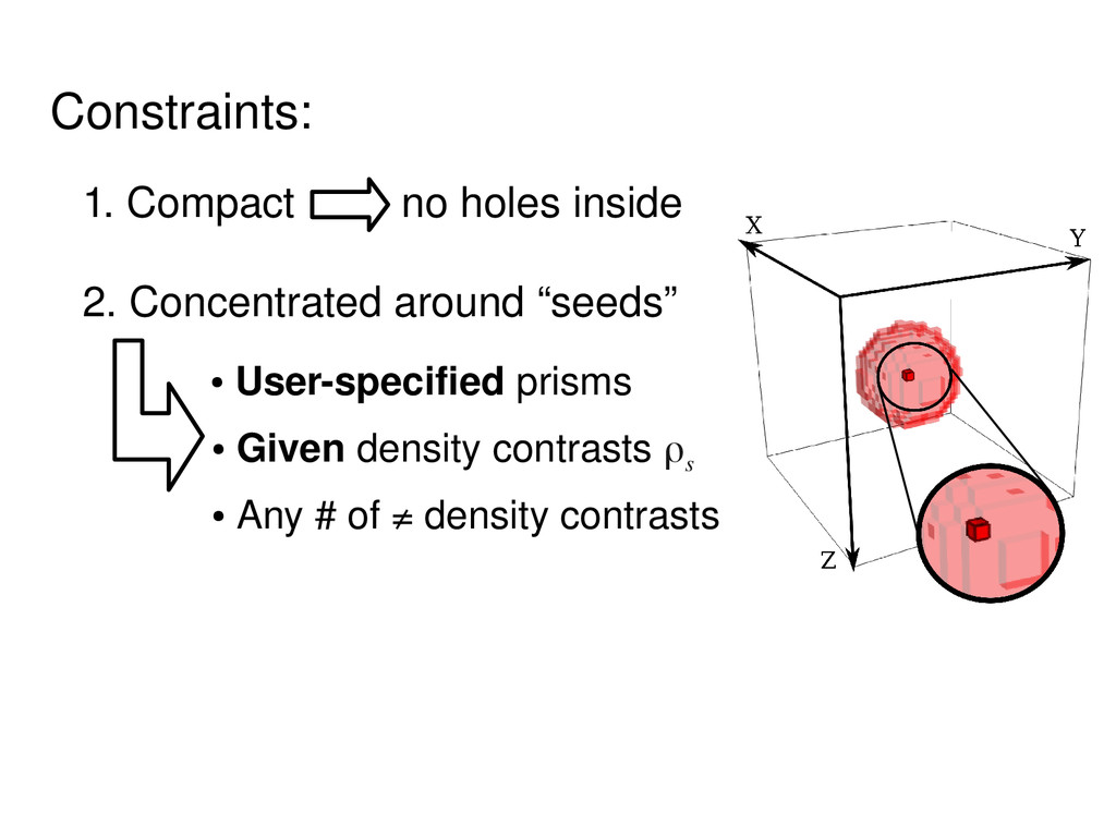
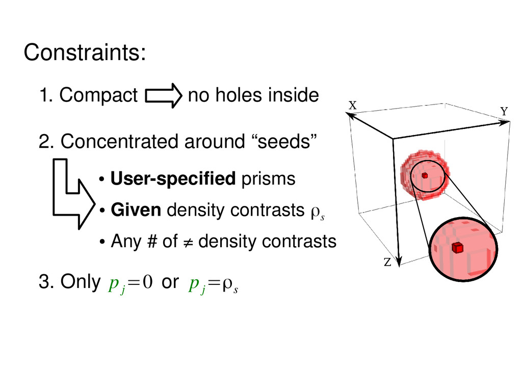
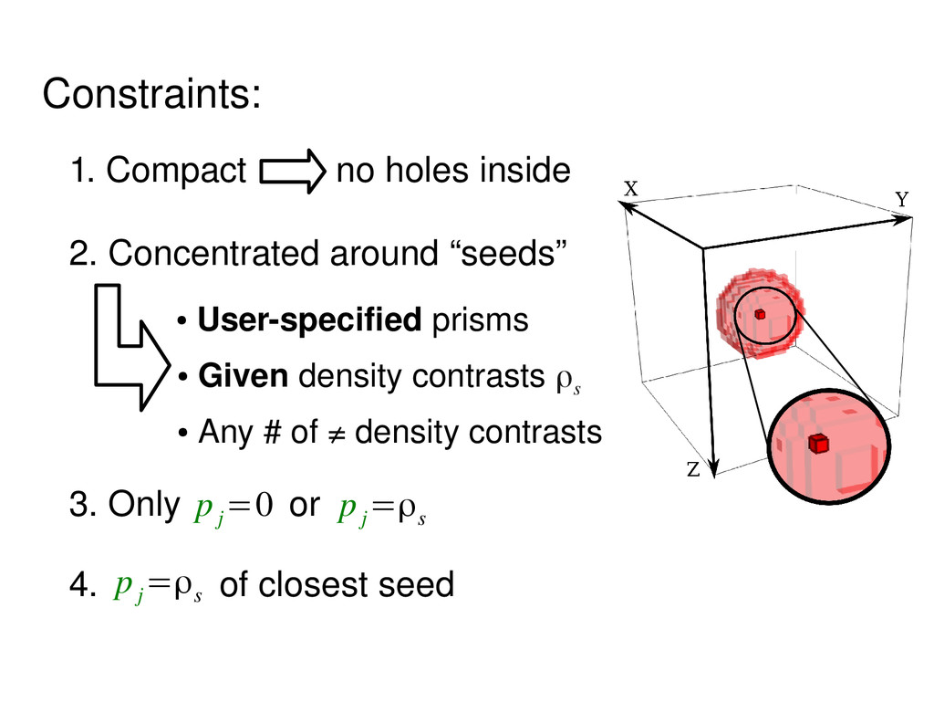
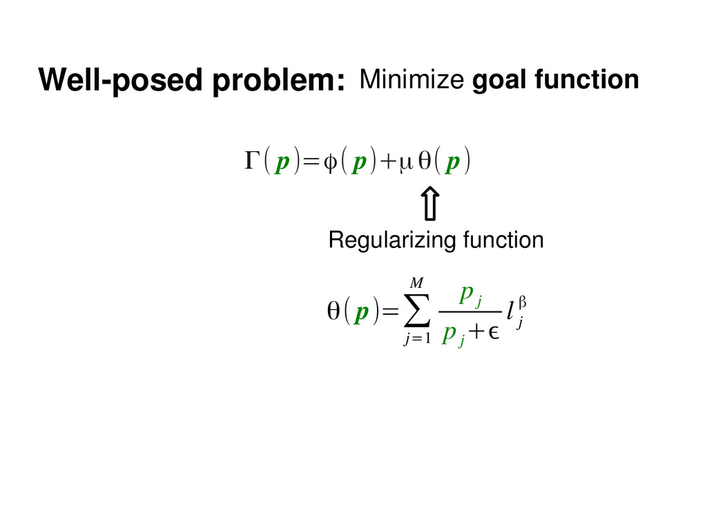
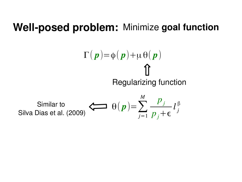
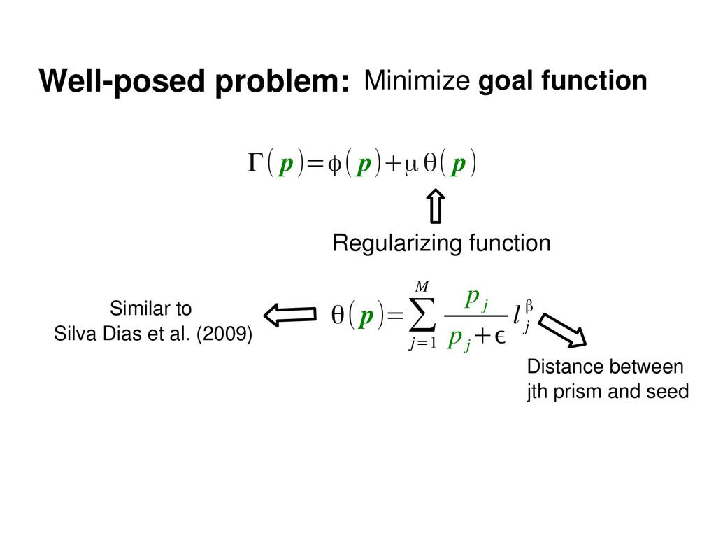
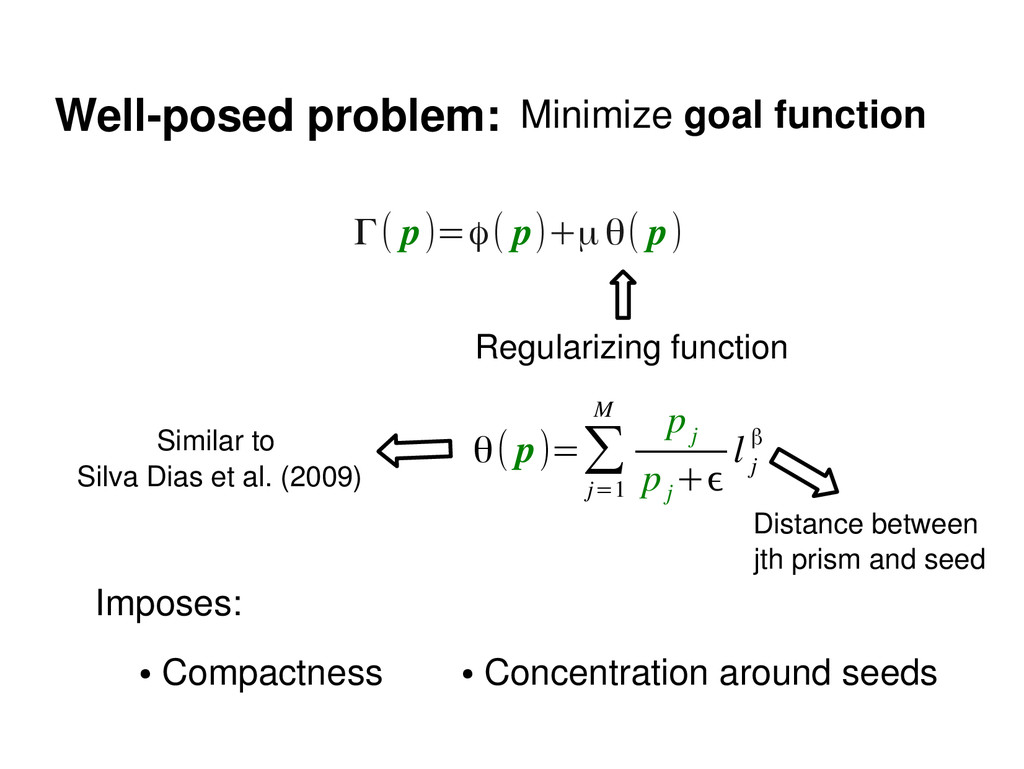
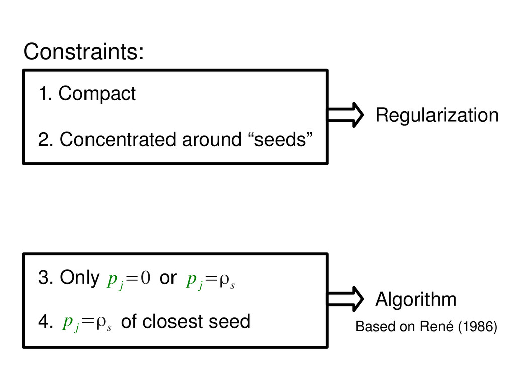
function θ( p)=∑ j=1 M p j p j +ϵ l j β Similar to Silva Dias et al. (2009) Distance between jth prism and seed Imposes: • Compactness • Concentration around seeds
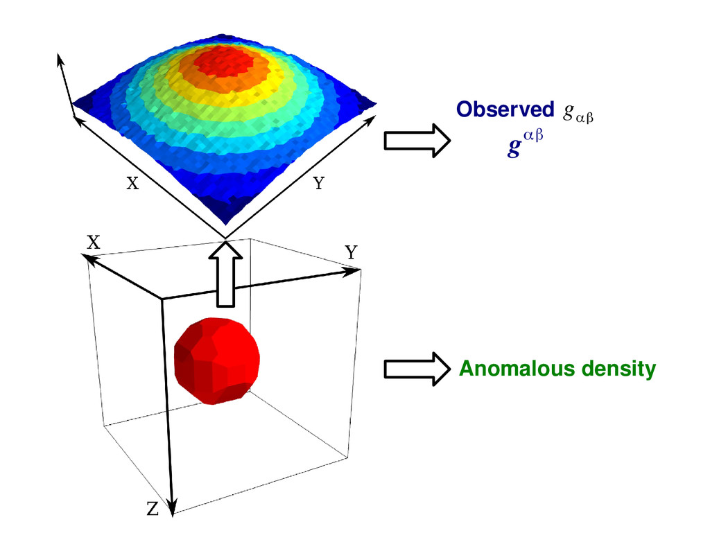
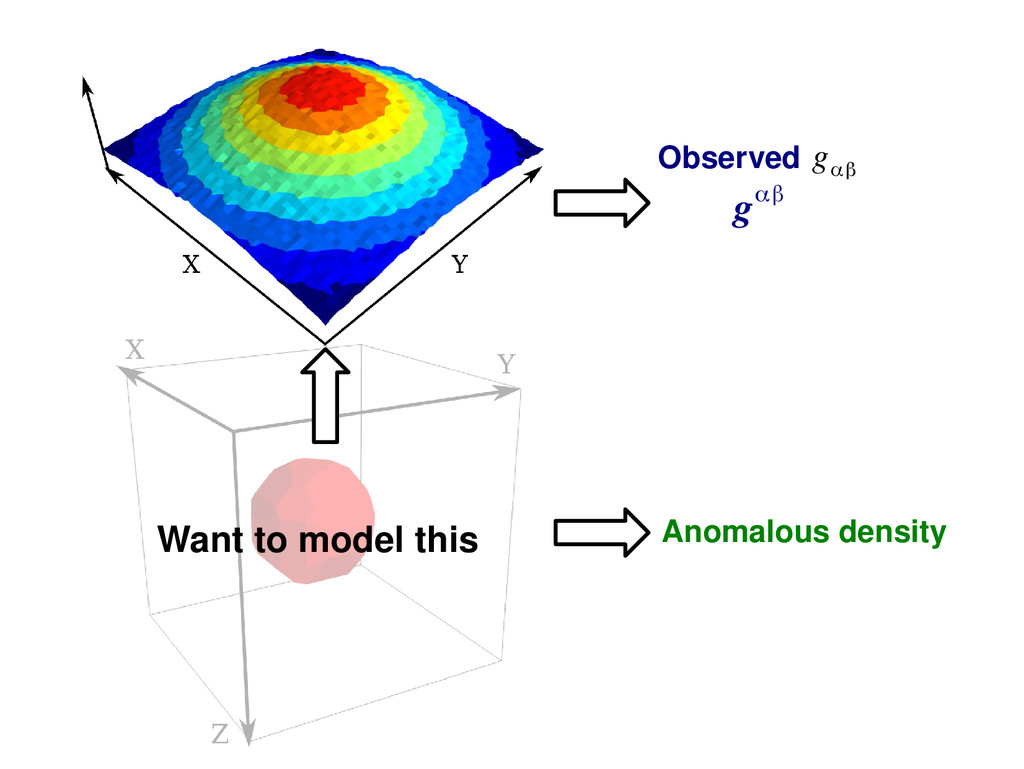
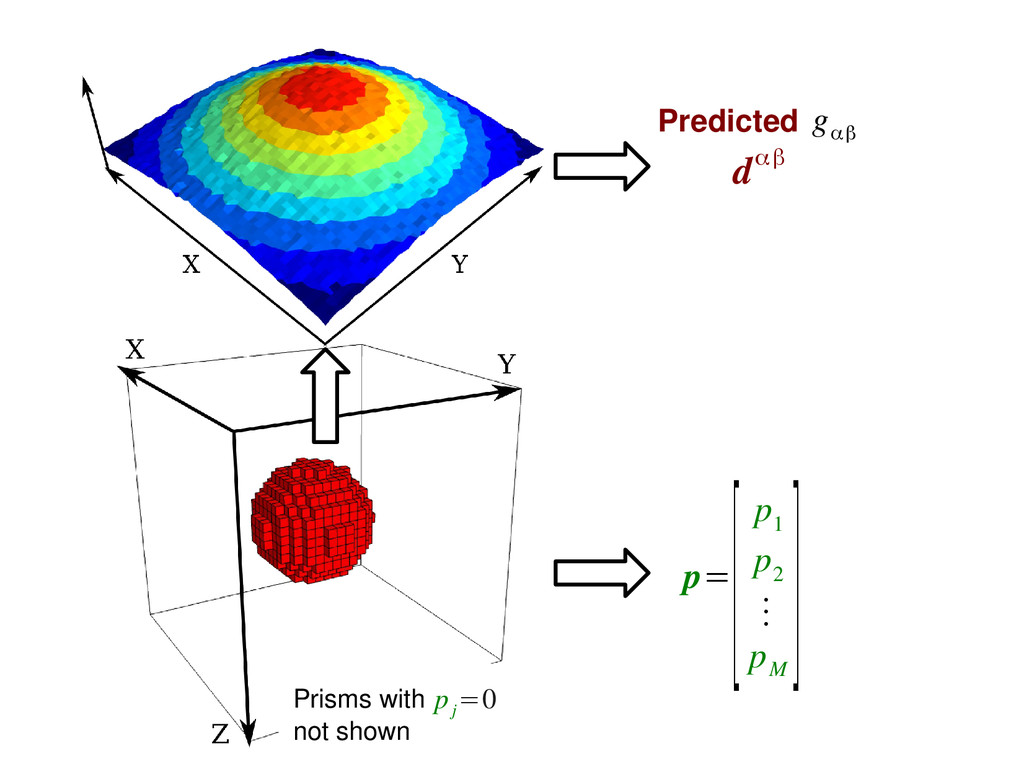
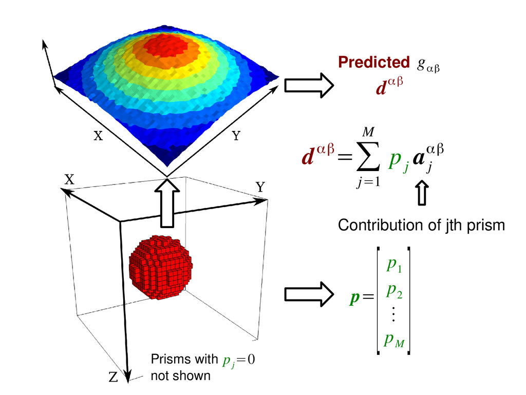
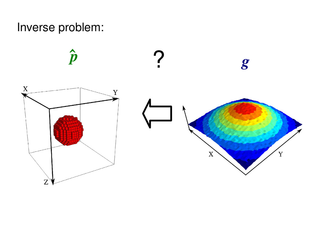
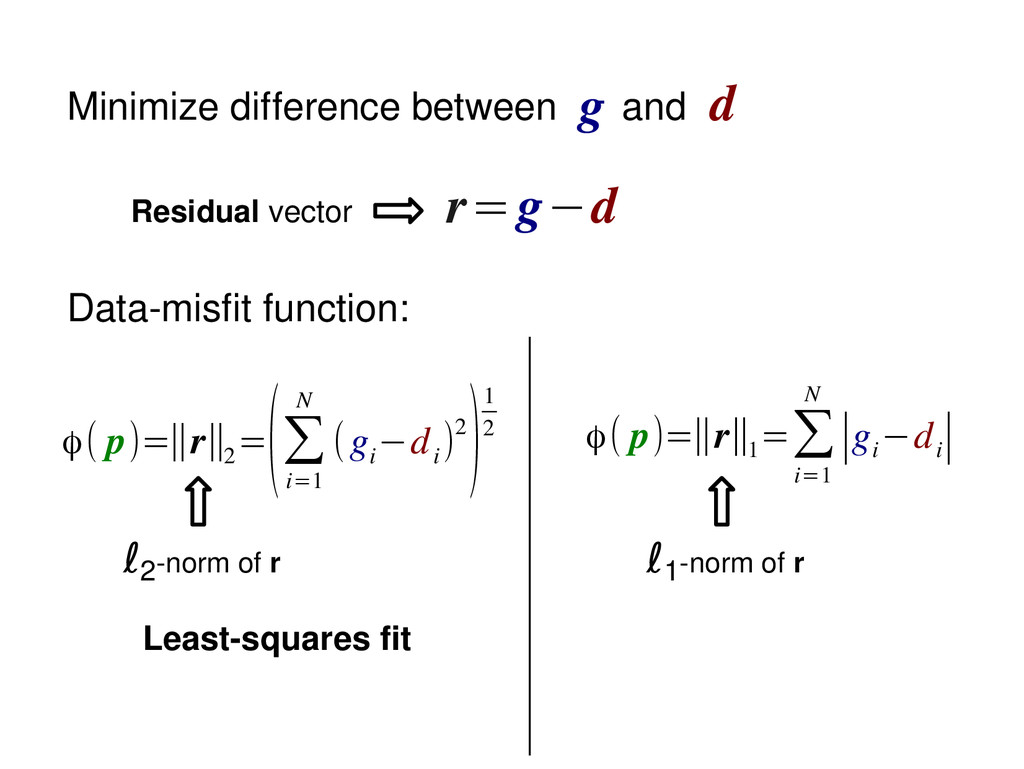
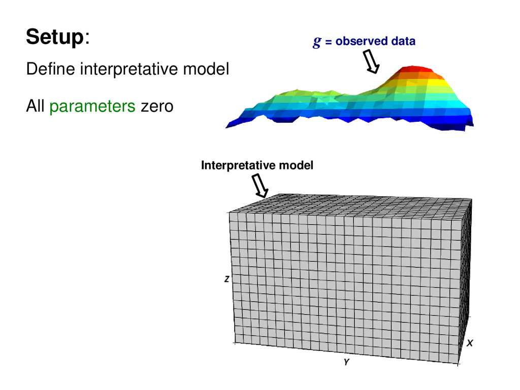
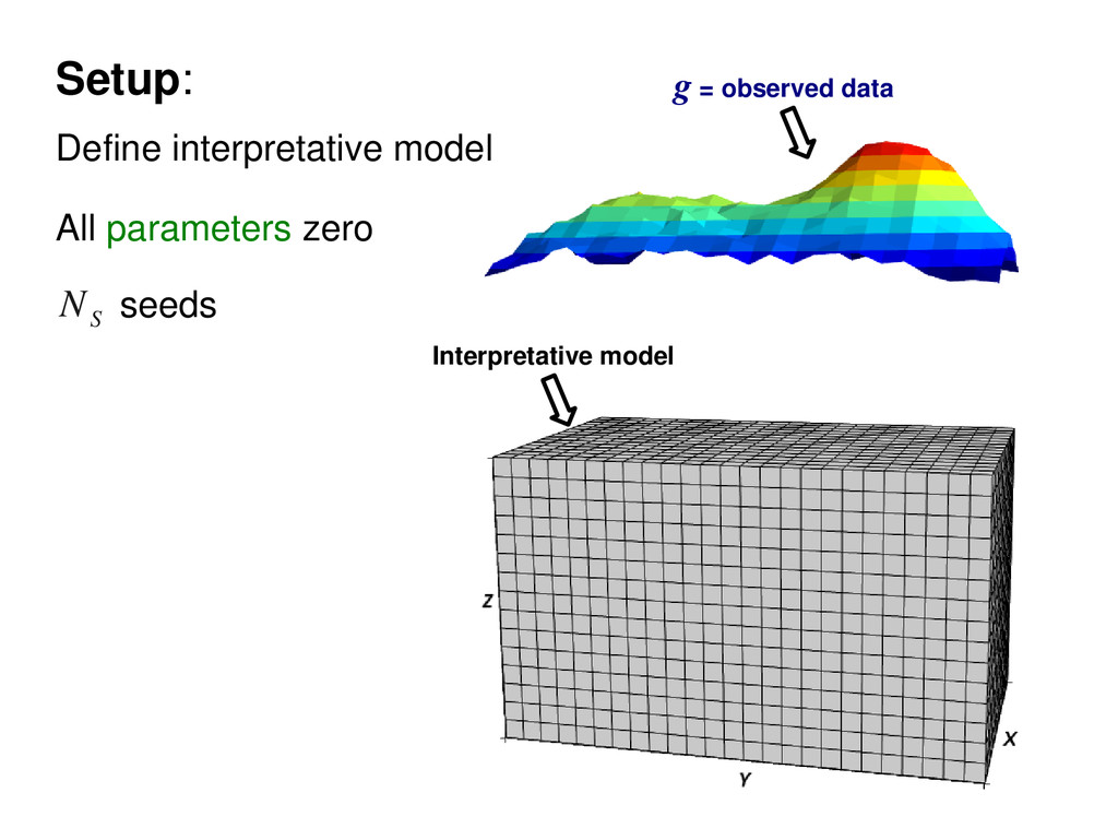
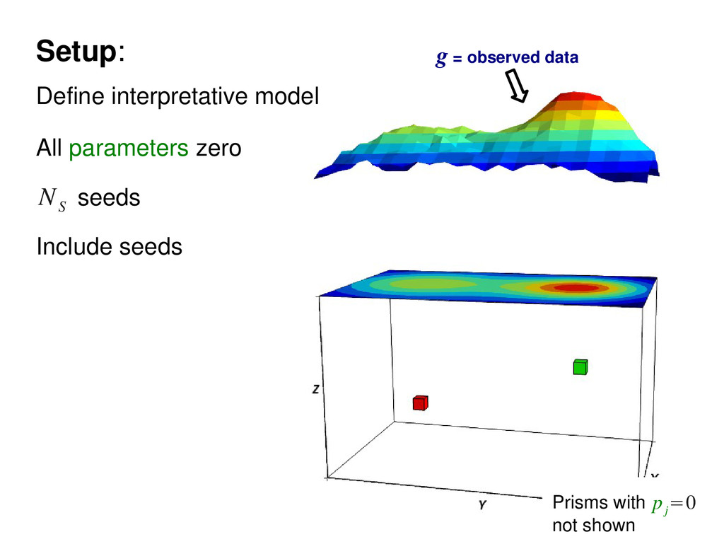
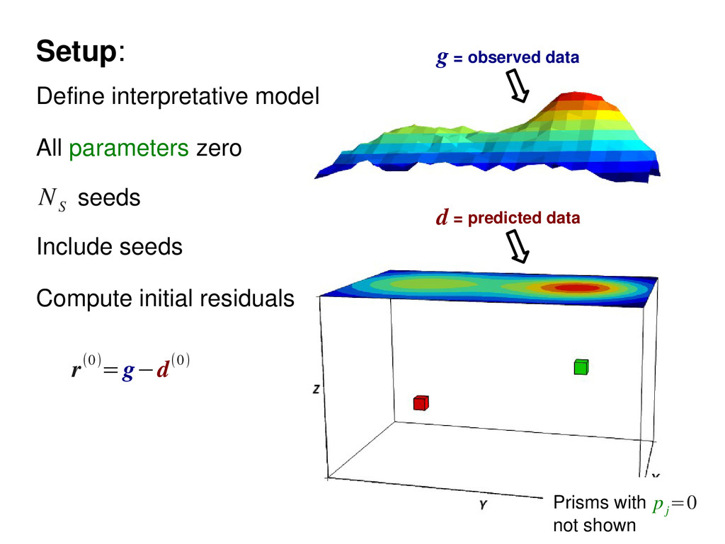
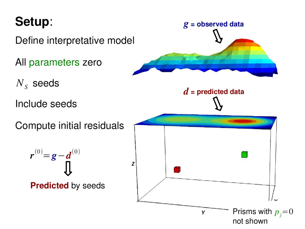
seeds Compute initial residuals r(0)=g− (∑ s=1 N S ρ s a j S ) Prisms with not shown g = observed data d = predicted data Neighbors Find neighbors of seeds p j =0 Setup:
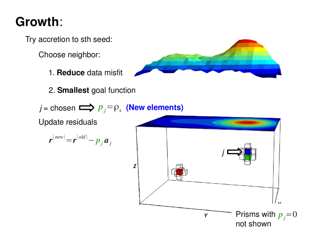
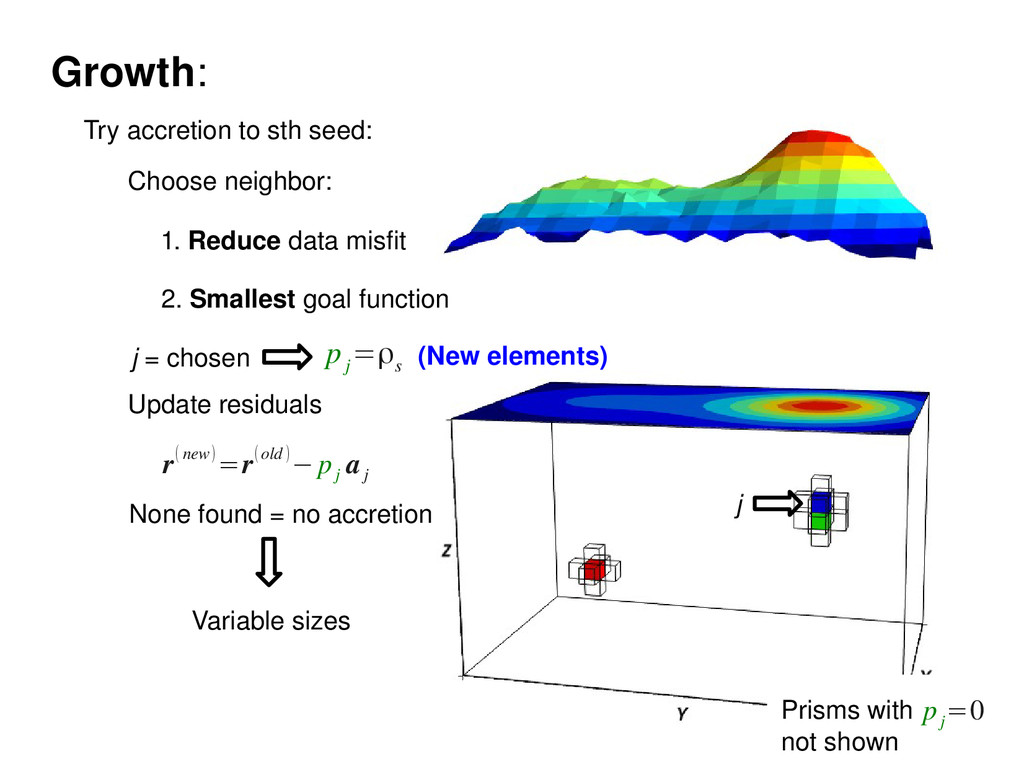
Reduce data misfit 2. Smallest goal function p j =ρ s j = chosen Choose neighbor: p j =0 Growth: (New elements) j Update residuals r(new)=r(old )− p j a j
Reduce data misfit 2. Smallest goal function p j =ρ s j = chosen Choose neighbor: p j =0 Growth: (New elements) j Update residuals r(new)=r(old )− p j a j Contribution of j
Reduce data misfit 2. Smallest goal function p j =ρ s j = chosen Choose neighbor: p j =0 Growth: (New elements) j Update residuals r(new)=r(old )− p j a j Variable sizes None found = no accretion
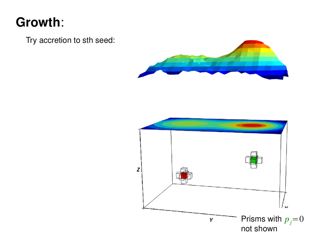
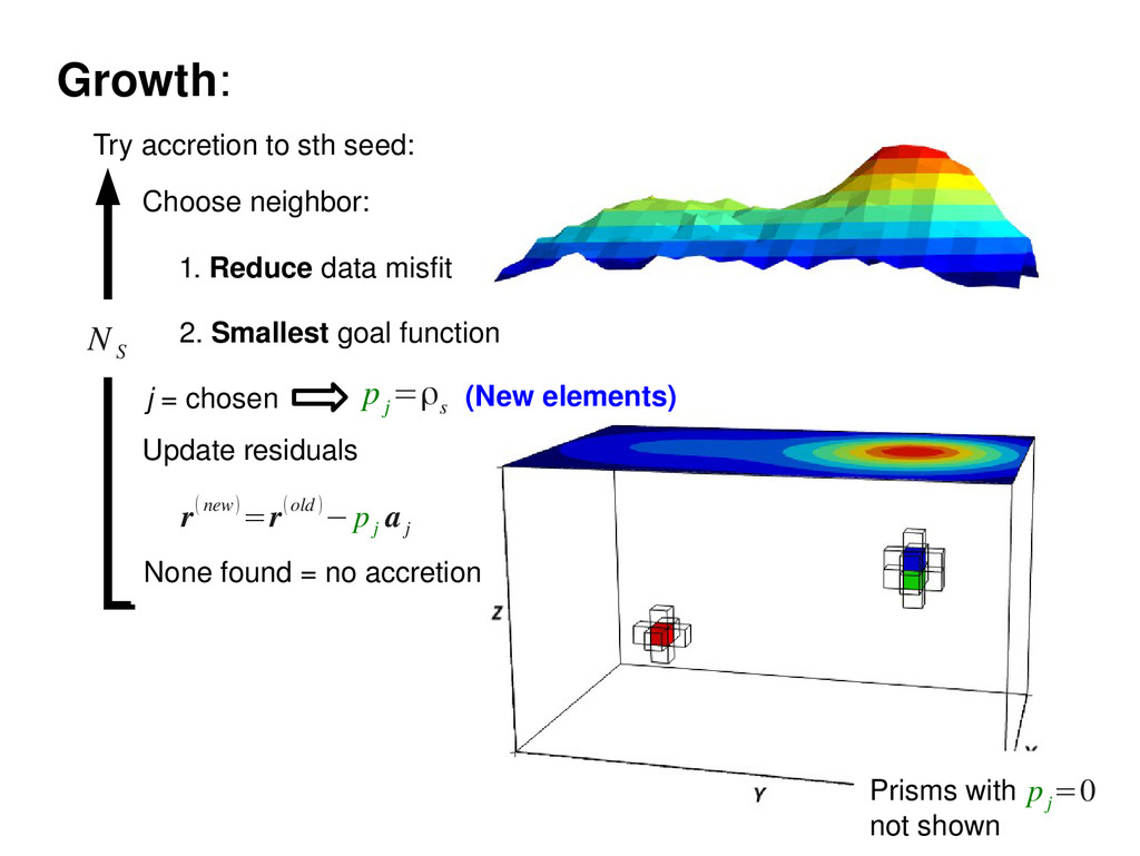
S Try accretion to sth seed: 1. Reduce data misfit 2. Smallest goal function p j =ρ s j = chosen Update residuals r(new)=r(old )− p j a j Choose neighbor: p j =0 Growth: (New elements)
S Try accretion to sth seed: 1. Reduce data misfit 2. Smallest goal function p j =ρ s j = chosen Update residuals r(new)=r(old )− p j a j Choose neighbor: p j =0 Growth: j (New elements)
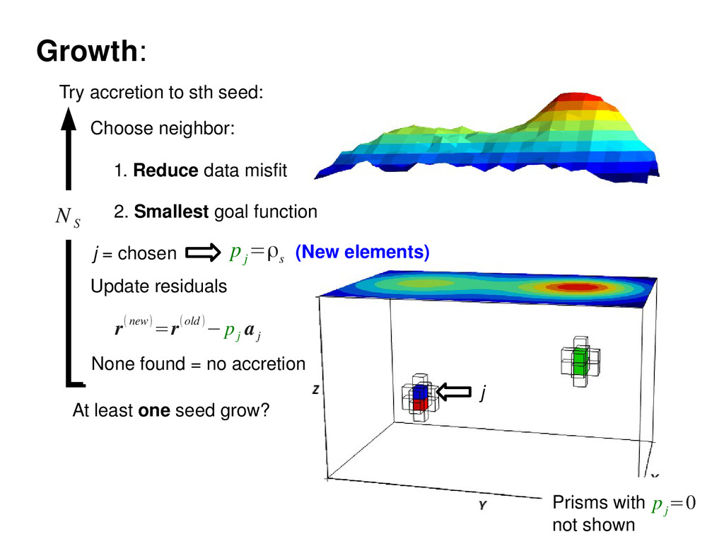
S Try accretion to sth seed: 1. Reduce data misfit 2. Smallest goal function p j =ρ s j = chosen Update residuals r(new)=r(old )− p j a j Choose neighbor: At least one seed grow? p j =0 Growth: j (New elements)
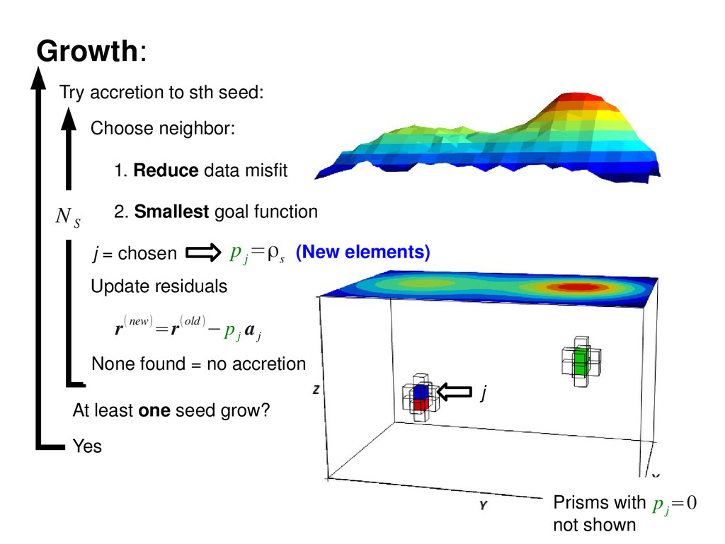
S Try accretion to sth seed: 1. Reduce data misfit 2. Smallest goal function p j =ρ s j = chosen Update residuals r(new)=r(old )− p j a j Choose neighbor: At least one seed grow? Yes p j =0 Growth: j (New elements)
S Try accretion to sth seed: 1. Reduce data misfit 2. Smallest goal function p j =ρ s j = chosen Update residuals r(new)=r(old )− p j a j Choose neighbor: At least one seed grow? Yes No p j =0 Growth: Done! j (New elements)
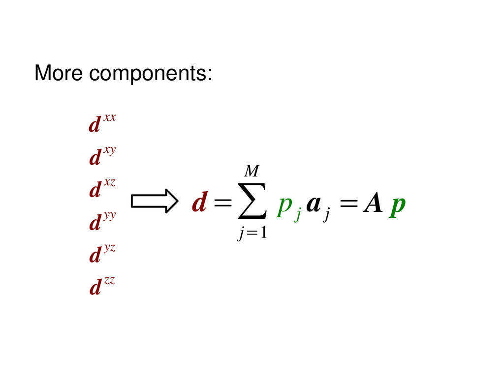
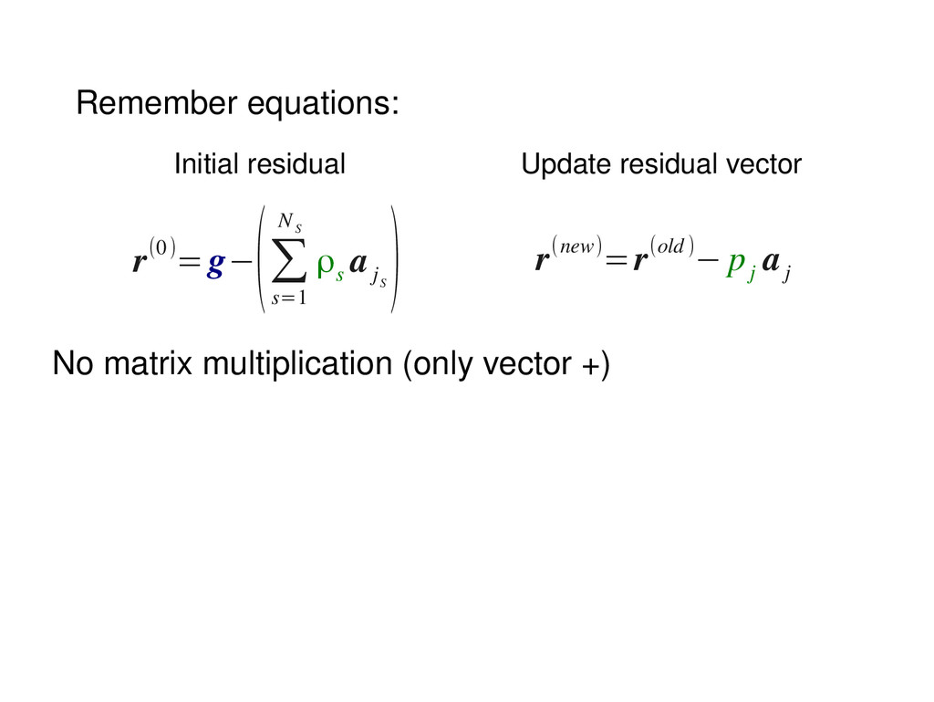
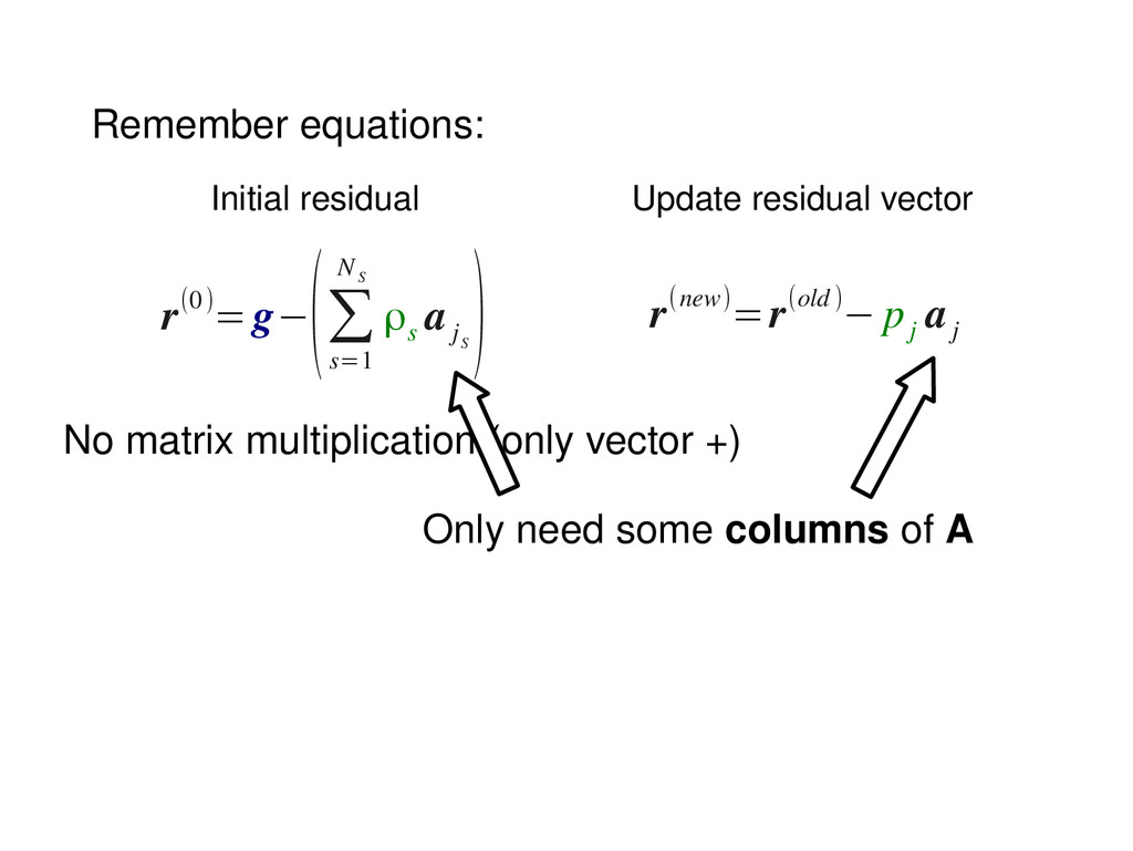
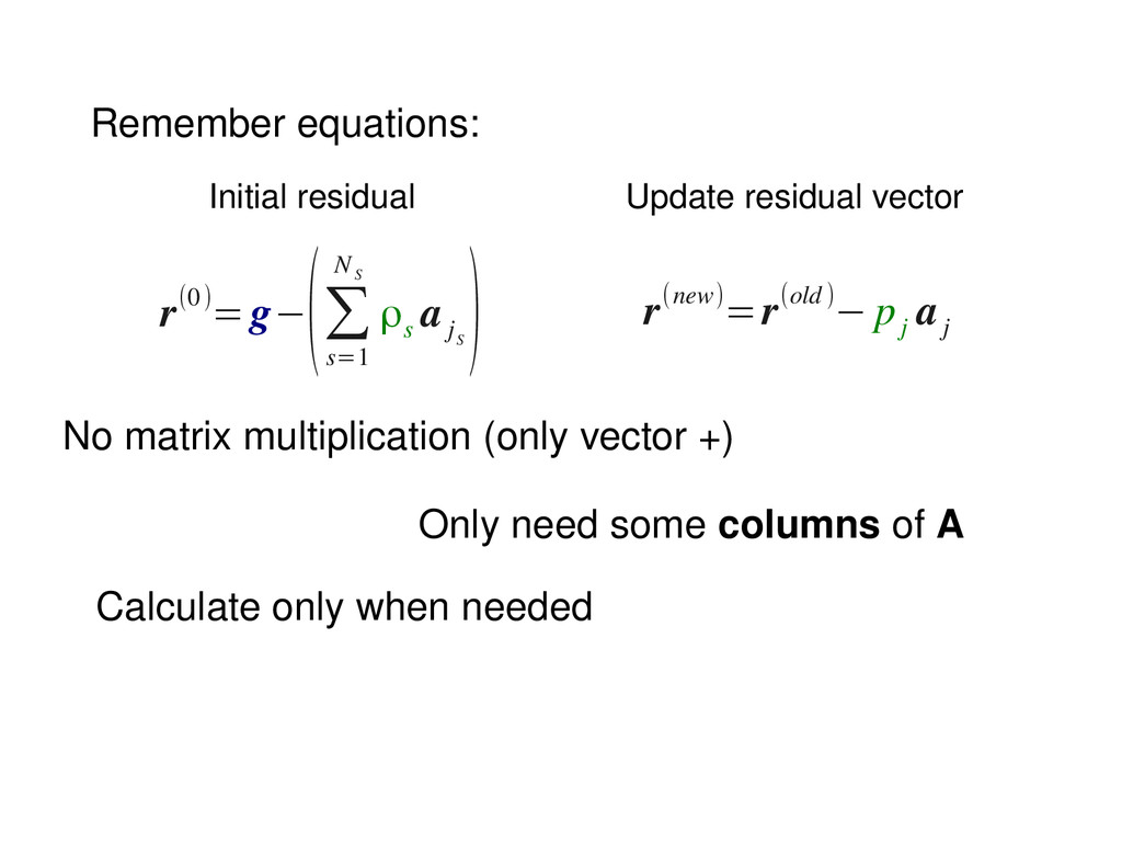
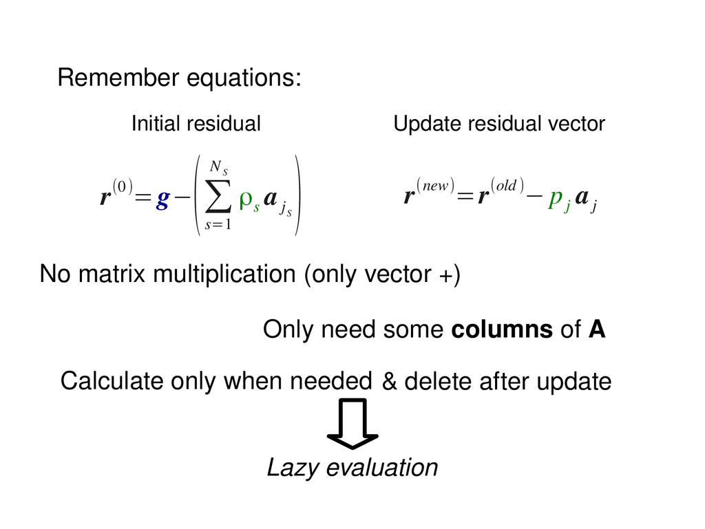
s=1 N S ρ s a j S ) r(new)=r(old)− p j a j Initial residual Update residual vector Only need some columns of A Calculate only when needed & delete after update
s=1 N S ρ s a j S ) r(new)=r(old)− p j a j Initial residual Update residual vector Only need some columns of A Calculate only when needed Lazy evaluation & delete after update
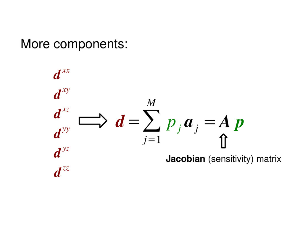
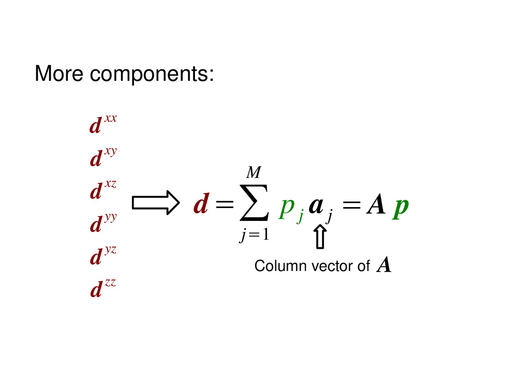
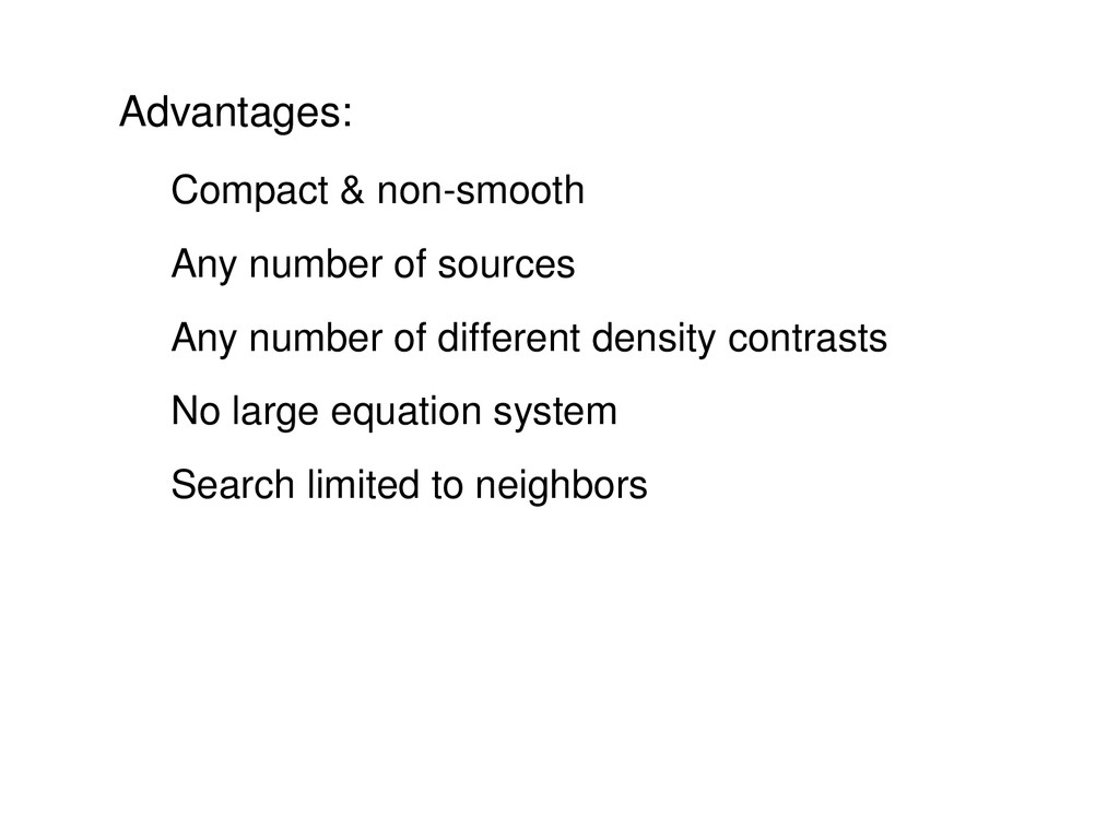
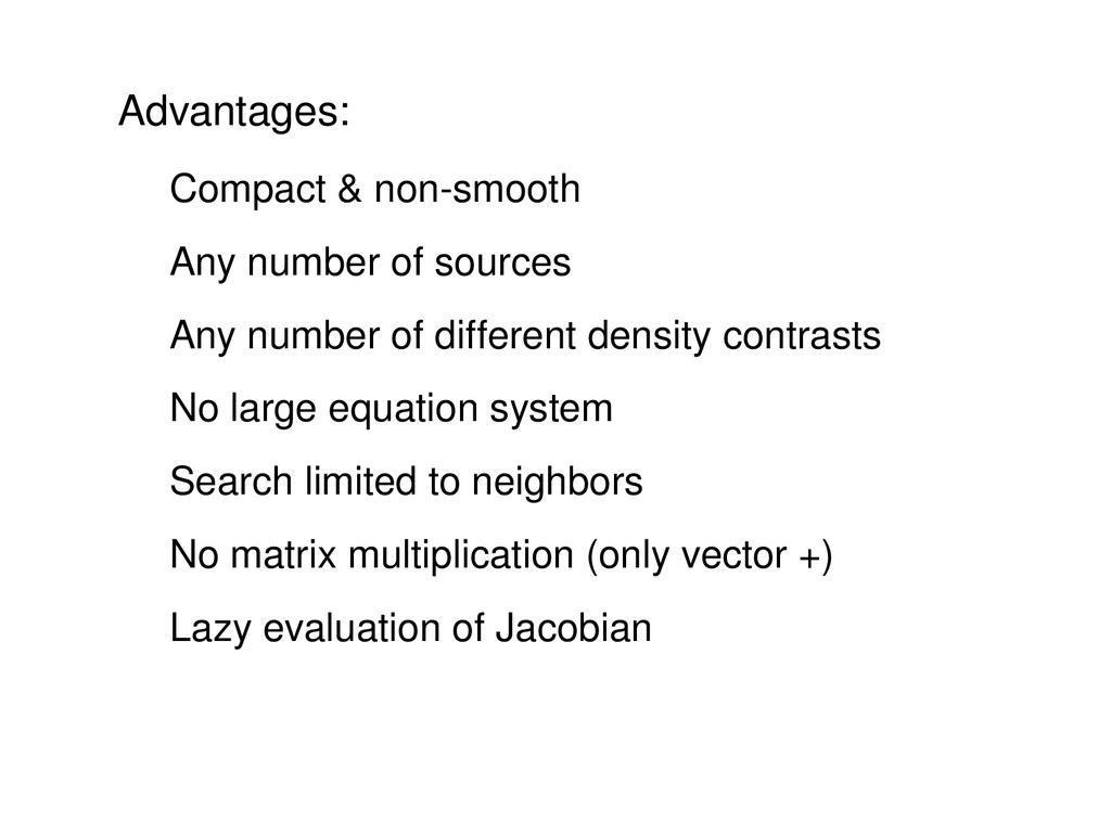
of different density contrasts No large equation system Search limited to neighbors No matrix multiplication (only vector +) Lazy evaluation of Jacobian
of different density contrasts No large equation system Search limited to neighbors No matrix multiplication (only vector +) Lazy evaluation of Jacobian Fast inversion + low memory usage
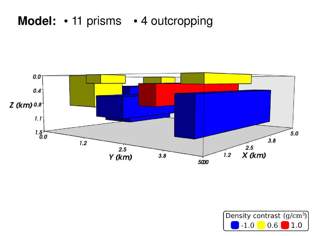
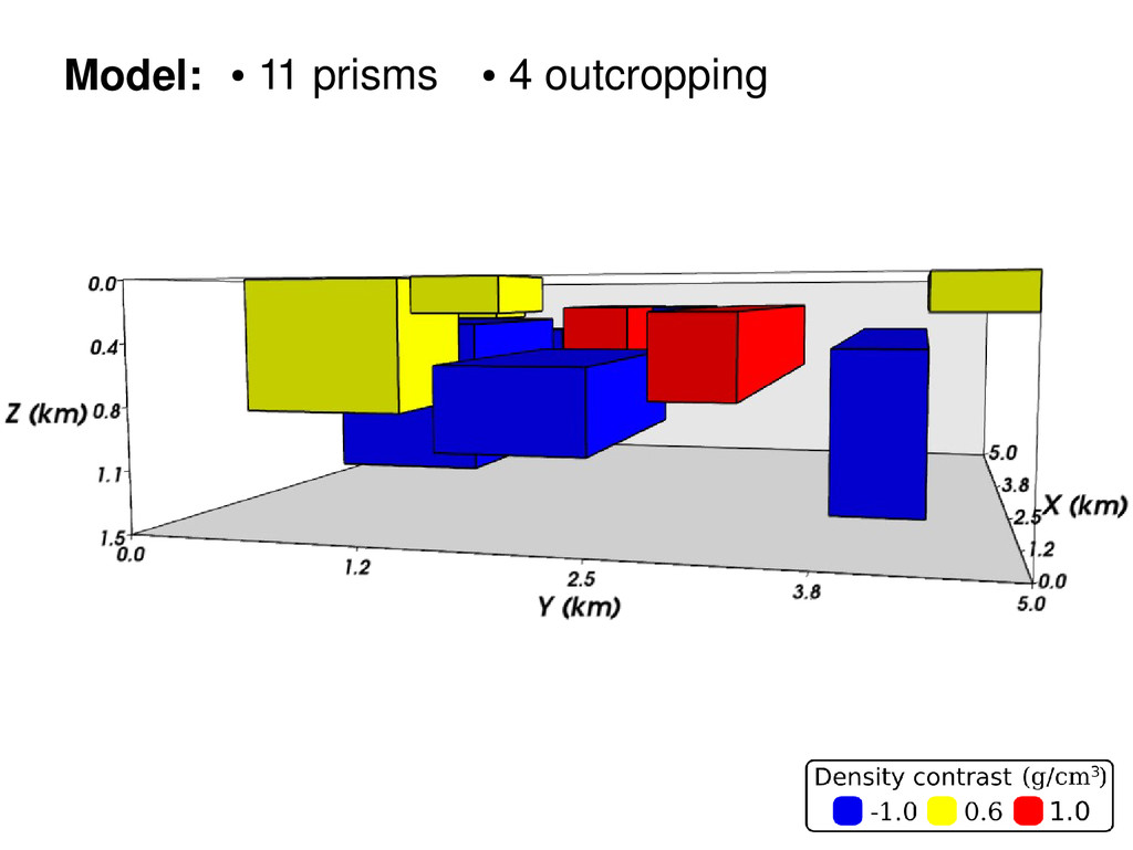
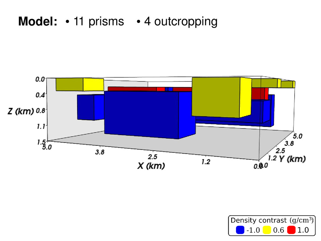
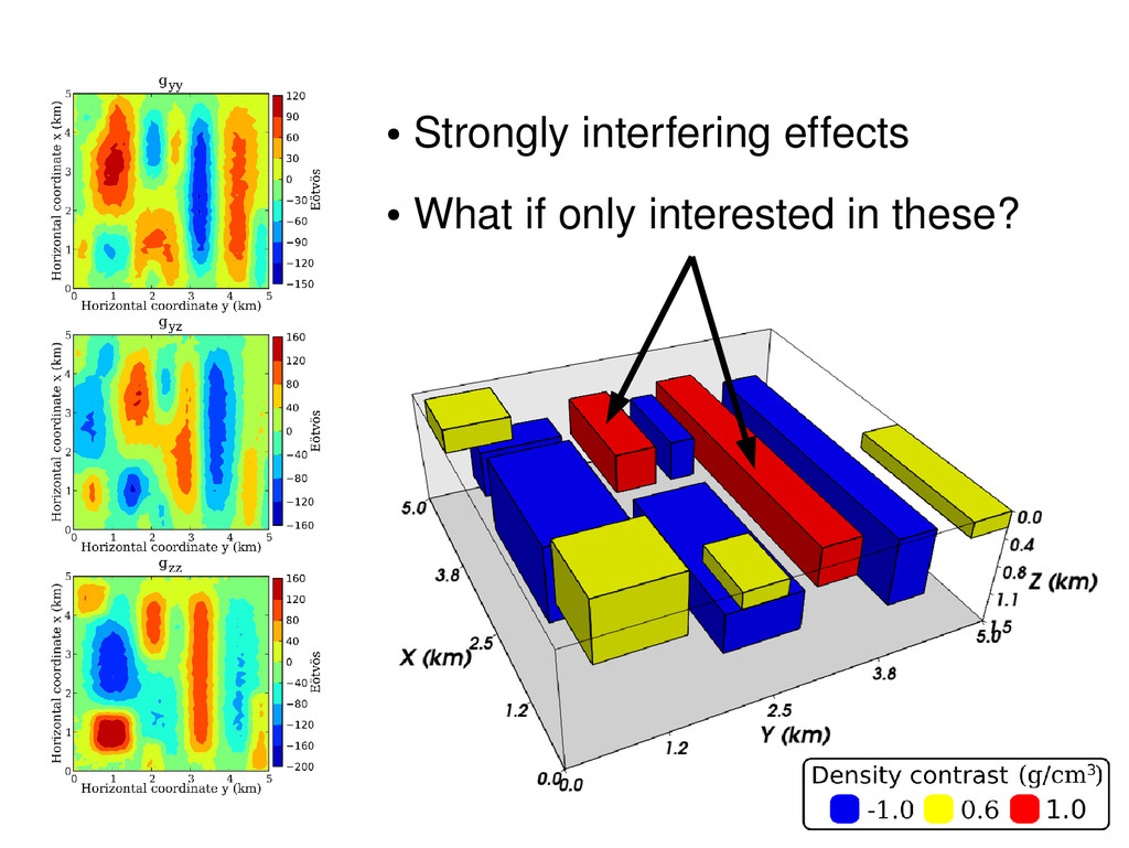
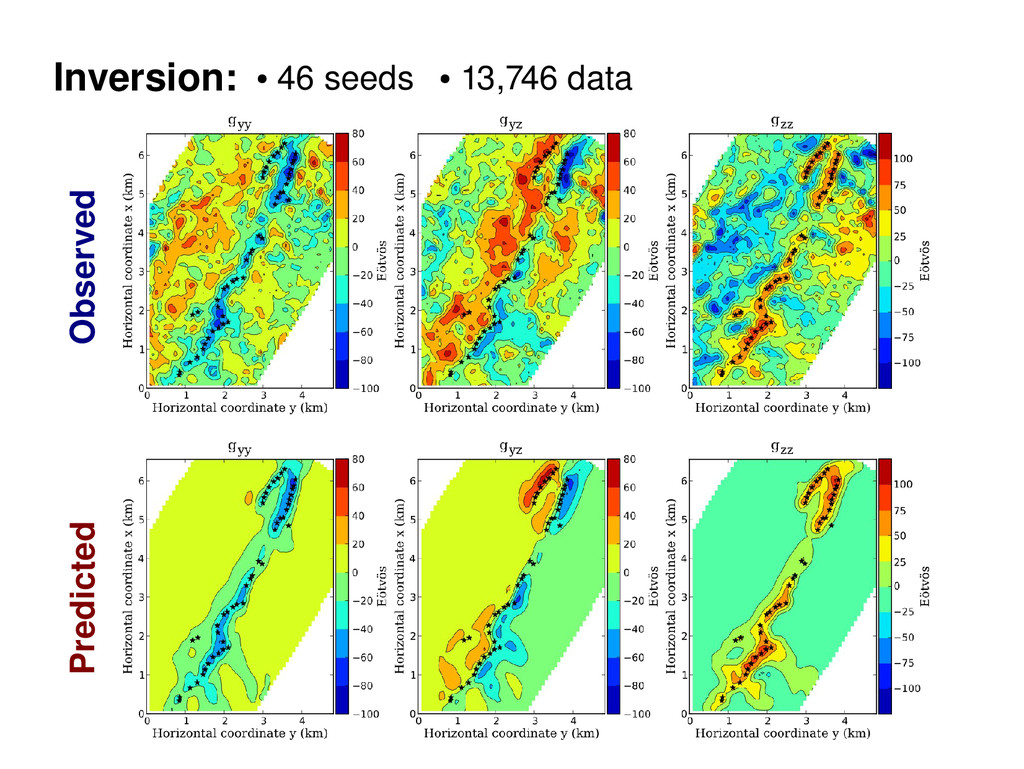
Interfering gravitational effects • Nontargeted sources • No matrix multiplications • No linear systems • Lazy evaluation of Jacobian matrix Conclusions
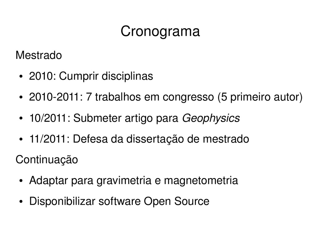
congresso (5 primeiro autor) • 10/2011: Submeter artigo para Geophysics • 11/2011: Defesa da dissertação de mestrado Continuação • Adaptar para gravimetria e magnetometria • Disponibilizar software Open Source Cronograma
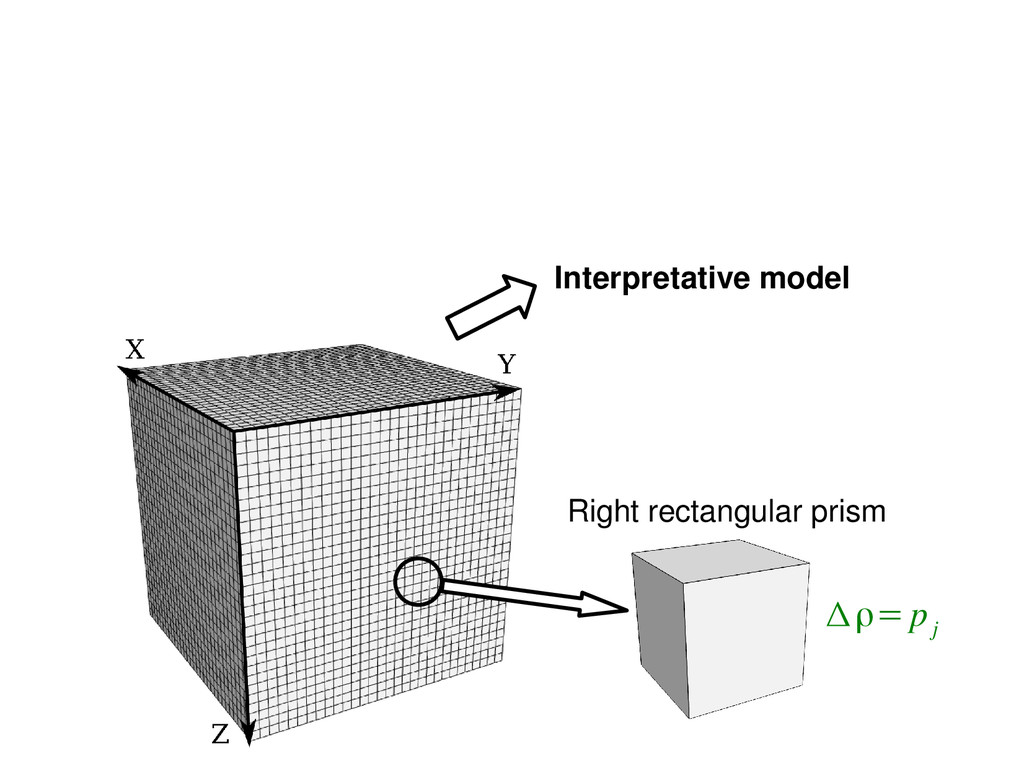
![p= [p 1 p 2 ⋮ p M ] Prisms](https://files.speakerdeck.com/presentations/6152ff6f20e749c891c92f79779bc6fb/slide_15.jpg)