Digital Pathology - MICCAI 2012

Transcript

1. Computerized Image Analysis in Digital Pathology with Histological and Cytological Virtual Slides Olivier L´ ezoray Universit´ e de Caen Basse Normandie olivier.lezoray@unicaen.fr http://lezoray.users.greyc.fr
2. 1 Introduction 2 Regularization on graphs 3 Multi-resolution Segmentation Methods of Breast and Equine Tendon Histological WSI 4 High-content screening in cytological digital slides O. L´ ezoray (University of Caen) 2 / 63
3. 1 Introduction 2 Regularization on graphs 3 Multi-resolution Segmentation Methods of Breast and Equine Tendon Histological WSI 4 High-content screening in cytological digital slides O. L´ ezoray (University of Caen) 3 / 63
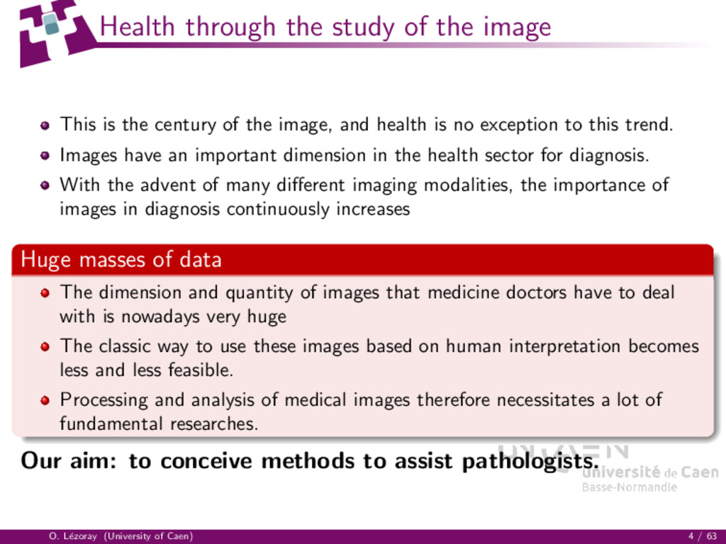
4. Health through the study of the image This is the century of the image, and health is no exception to this trend. Images have an important dimension in the health sector for diagnosis. With the advent of many different imaging modalities, the importance of images in diagnosis continuously increases Huge masses of data The dimension and quantity of images that medicine doctors have to deal with is nowadays very huge The classic way to use these images based on human interpretation becomes less and less feasible. Processing and analysis of medical images therefore necessitates a lot of fundamental researches. Our aim: to conceive methods to assist pathologists. O. L´ ezoray (University of Caen) 4 / 63
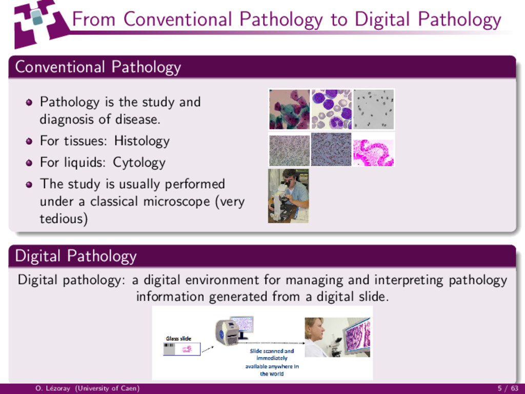
5. From Conventional Pathology to Digital Pathology Conventional Pathology Pathology is the study and diagnosis of disease. For tissues: Histology For liquids: Cytology The study is usually performed under a classical microscope (very tedious) Digital Pathology Digital pathology: a digital environment for managing and interpreting pathology information generated from a digital slide. O. L´ ezoray (University of Caen) 5 / 63
6. Computer Aided Diagnosis – Digital Pathology O. L´ ezoray (University of Caen) 6 / 63
7. What we will talk about A theoretical framework for the processing of images as graphs This provides a set of efficient tools for microscopic image processing and analysis (mainly for filtering and segmentation) Applications of digital slide image analysis in histopathology and cytology Mitosis extraction in breast cancer histological digital slides Tendon structure analysis in histological digital slides of equine tendinopathy High-content screening in cytological digital slides for early diagnosis of mesothelioma in serous samples O. L´ ezoray (University of Caen) 7 / 63
8. 1 Introduction 2 Regularization on graphs Processing graphs signals Weighted graphs Basics Operators on graphs p-Laplacian regularization on graphs 3 Multi-resolution Segmentation Methods of Breast and Equine Tendon Histological WSI 4 High-content screening in cytological digital slides O. L´ ezoray (University of Caen) 8 / 63
9. 1 Introduction 2 Regularization on graphs Processing graphs signals Weighted graphs Basics Operators on graphs p-Laplacian regularization on graphs 3 Multi-resolution Segmentation Methods of Breast and Equine Tendon Histological WSI Multi-resolution Segmentation Method of Breast Histological WSI Image Analysis Method of Equine Tendon Histological WSI 4 High-content screening in cytological digital slides O. L´ ezoray (University of Caen) 9 / 63
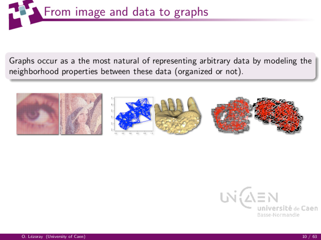
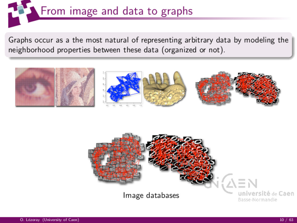
10. From image and data to graphs Graphs occur as a the most natural of representing arbitrary data by modeling the neighborhood properties between these data (organized or not). 0.0 0.2 0.4 0.6 0.8 1.0 0.0 0.2 0.4 0.6 0.8 1.0 O. L´ ezoray (University of Caen) 10 / 63
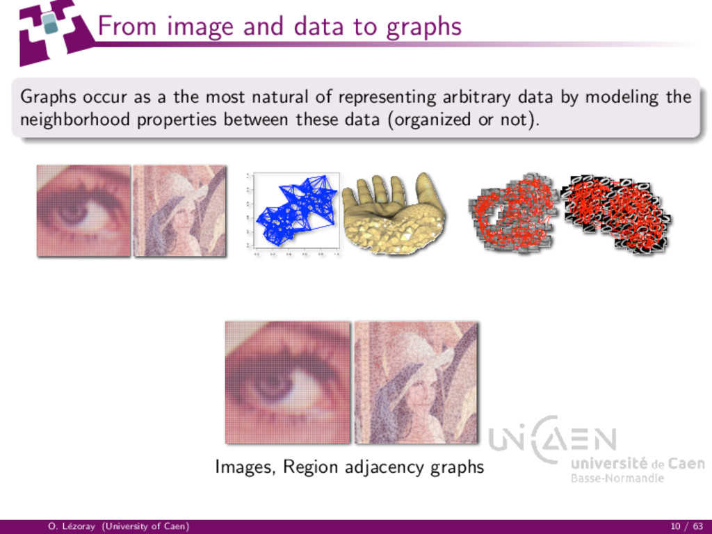
11. From image and data to graphs Graphs occur as a the most natural of representing arbitrary data by modeling the neighborhood properties between these data (organized or not). 0.0 0.2 0.4 0.6 0.8 1.0 0.0 0.2 0.4 0.6 0.8 1.0 Images, Region adjacency graphs O. L´ ezoray (University of Caen) 10 / 63
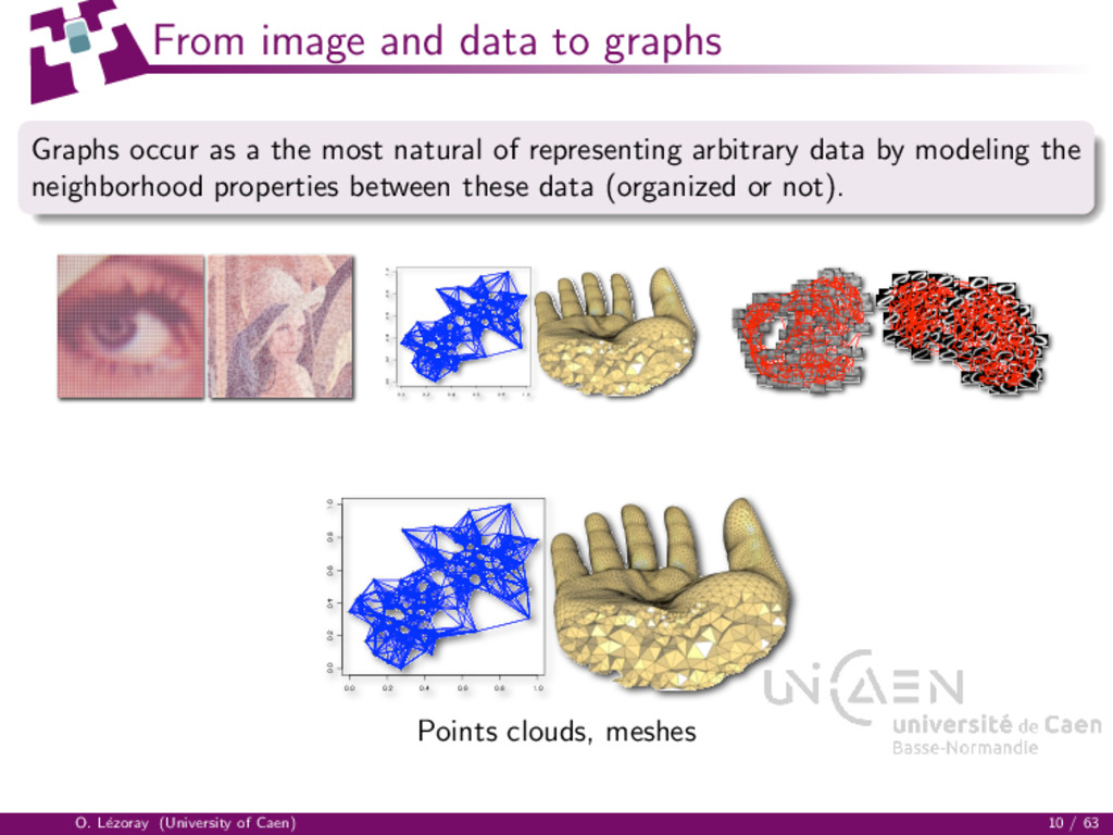
12. From image and data to graphs Graphs occur as a the most natural of representing arbitrary data by modeling the neighborhood properties between these data (organized or not). 0.0 0.2 0.4 0.6 0.8 1.0 0.0 0.2 0.4 0.6 0.8 1.0 0.0 0.2 0.4 0.6 0.8 1.0 0.0 0.2 0.4 0.6 0.8 1.0 Points clouds, meshes O. L´ ezoray (University of Caen) 10 / 63
13. From image and data to graphs Graphs occur as a the most natural of representing arbitrary data by modeling the neighborhood properties between these data (organized or not). 0.0 0.2 0.4 0.6 0.8 1.0 0.0 0.2 0.4 0.6 0.8 1.0 Image databases O. L´ ezoray (University of Caen) 10 / 63
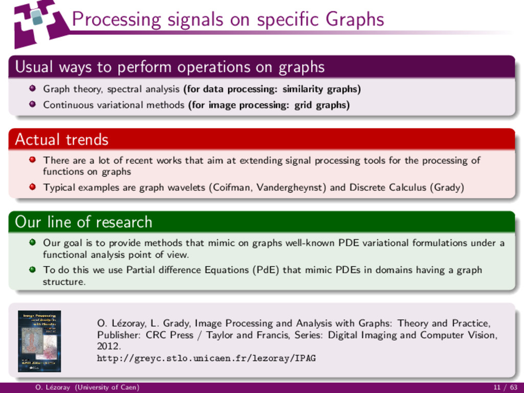
14. Processing signals on specific Graphs Usual ways to perform operations on graphs Graph theory, spectral analysis (for data processing: similarity graphs) Continuous variational methods (for image processing: grid graphs) Actual trends There are a lot of recent works that aim at extending signal processing tools for the processing of functions on graphs Typical examples are graph wavelets (Coifman, Vandergheynst) and Discrete Calculus (Grady) Our line of research Our goal is to provide methods that mimic on graphs well-known PDE variational formulations under a functional analysis point of view. To do this we use Partial difference Equations (PdE) that mimic PDEs in domains having a graph structure. O. L´ ezoray, L. Grady, Image Processing and Analysis with Graphs: Theory and Practice, Publisher: CRC Press / Taylor and Francis, Series: Digital Imaging and Computer Vision, 2012. http://greyc.stlo.unicaen.fr/lezoray/IPAG O. L´ ezoray (University of Caen) 11 / 63
15. 1 Introduction 2 Regularization on graphs Processing graphs signals Weighted graphs Basics Operators on graphs p-Laplacian regularization on graphs 3 Multi-resolution Segmentation Methods of Breast and Equine Tendon Histological WSI Multi-resolution Segmentation Method of Breast Histological WSI Image Analysis Method of Equine Tendon Histological WSI 4 High-content screening in cytological digital slides O. L´ ezoray (University of Caen) 12 / 63
16. Weighted graphs Basics A weighted graph G = (V, E, w) consists in a finite set V = {v1, . . . , vN } of N vertices O. L´ ezoray (University of Caen) 13 / 63
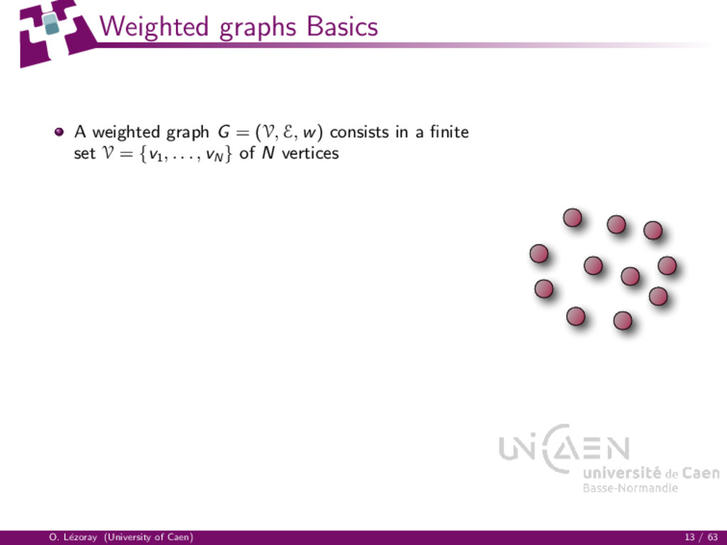
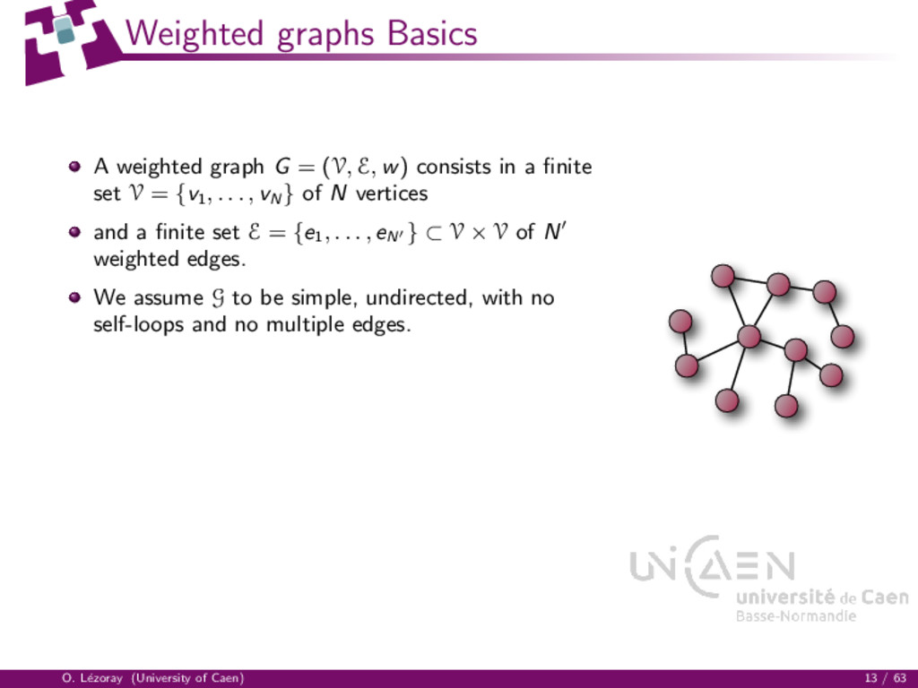
17. Weighted graphs Basics A weighted graph G = (V, E, w) consists in a finite set V = {v1, . . . , vN } of N vertices and a finite set E = {e1, . . . , eN } ⊂ V × V of N weighted edges. We assume G to be simple, undirected, with no self-loops and no multiple edges. O. L´ ezoray (University of Caen) 13 / 63
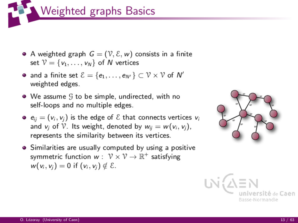
18. Weighted graphs Basics A weighted graph G = (V, E, w) consists in a finite set V = {v1, . . . , vN } of N vertices and a finite set E = {e1, . . . , eN } ⊂ V × V of N weighted edges. We assume G to be simple, undirected, with no self-loops and no multiple edges. eij = (vi , vj ) is the edge of E that connects vertices vi and vj of V. Its weight, denoted by wij = w(vi , vj ), represents the similarity between its vertices. Similarities are usually computed by using a positive symmetric function w : V × V → R+ satisfying w(vi , vj ) = 0 if (vi , vj ) / ∈ E. w w w w w w w w w w w O. L´ ezoray (University of Caen) 13 / 63
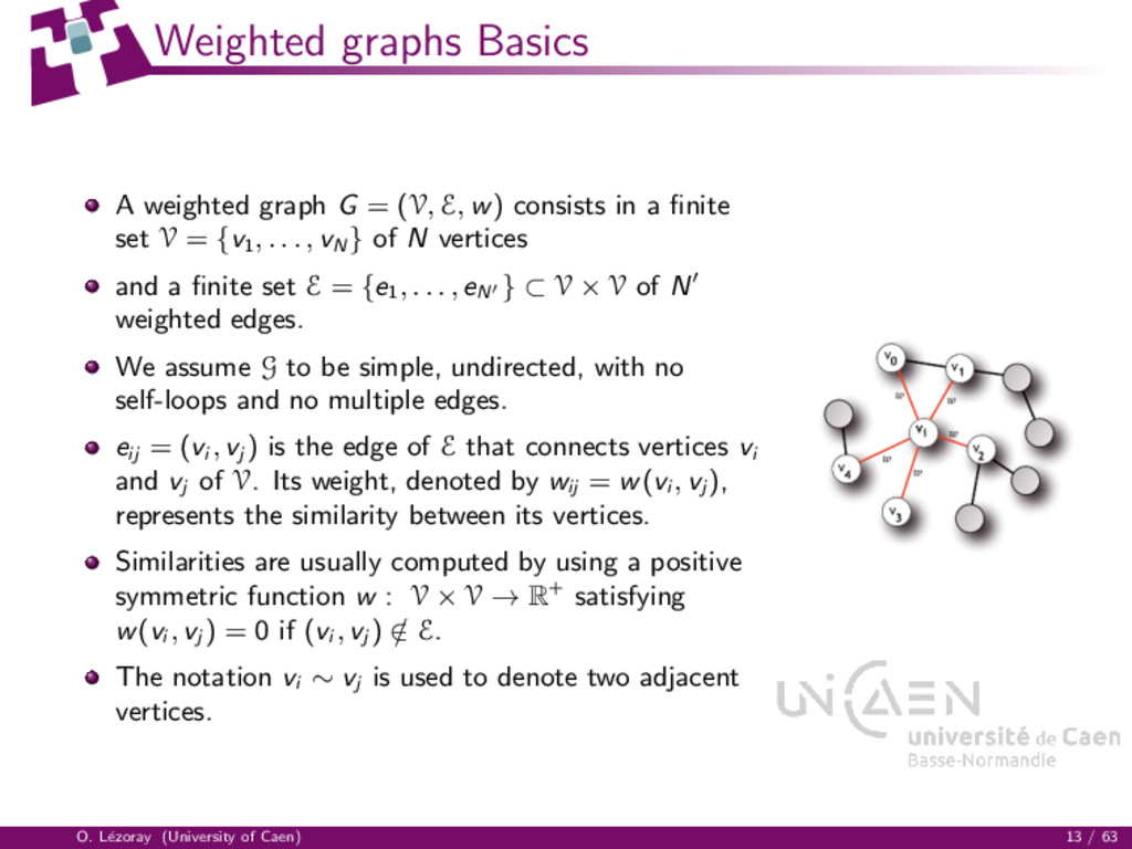
19. Weighted graphs Basics A weighted graph G = (V, E, w) consists in a finite set V = {v1, . . . , vN } of N vertices and a finite set E = {e1, . . . , eN } ⊂ V × V of N weighted edges. We assume G to be simple, undirected, with no self-loops and no multiple edges. eij = (vi , vj ) is the edge of E that connects vertices vi and vj of V. Its weight, denoted by wij = w(vi , vj ), represents the similarity between its vertices. Similarities are usually computed by using a positive symmetric function w : V × V → R+ satisfying w(vi , vj ) = 0 if (vi , vj ) / ∈ E. The notation vi ∼ vj is used to denote two adjacent vertices. O. L´ ezoray (University of Caen) 13 / 63
20. 1 Introduction 2 Regularization on graphs Processing graphs signals Weighted graphs Basics Operators on graphs p-Laplacian regularization on graphs 3 Multi-resolution Segmentation Methods of Breast and Equine Tendon Histological WSI Multi-resolution Segmentation Method of Breast Histological WSI Image Analysis Method of Equine Tendon Histological WSI 4 High-content screening in cytological digital slides O. L´ ezoray (University of Caen) 14 / 63
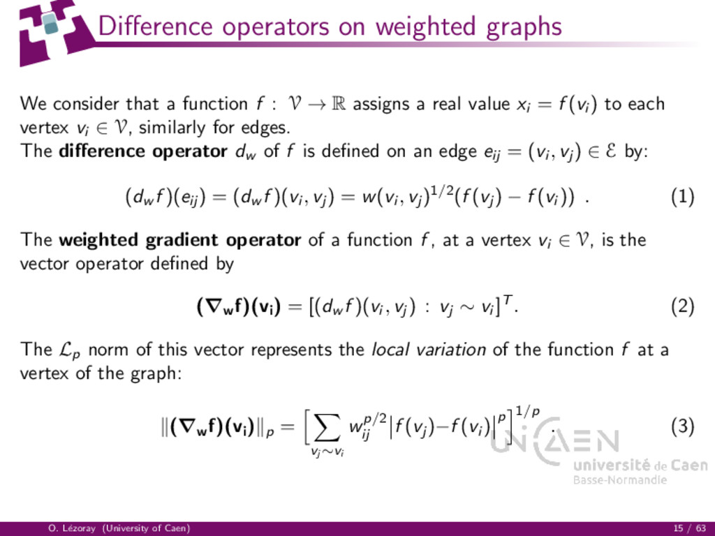
21. Difference operators on weighted graphs We consider that a function f : V → R assigns a real value xi = f (vi ) to each vertex vi ∈ V, similarly for edges. The difference operator dw of f is defined on an edge eij = (vi , vj ) ∈ E by: (dw f )(eij ) = (dw f )(vi , vj ) = w(vi , vj )1/2(f (vj ) − f (vi )) . (1) The weighted gradient operator of a function f , at a vertex vi ∈ V, is the vector operator defined by (∇w f)(vi ) = [(dw f )(vi , vj ) : vj ∼ vi ]T . (2) The Lp norm of this vector represents the local variation of the function f at a vertex of the graph: (∇w f)(vi ) p = vj ∼vi wp/2 ij f (vj )−f (vi ) p 1/p . (3) O. L´ ezoray (University of Caen) 15 / 63
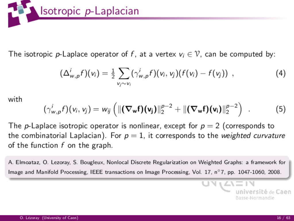
22. Isotropic p-Laplacian The isotropic p-Laplace operator of f , at a vertex vi ∈ V, can be computed by: (∆i w,p f )(vi ) = 1 2 vj ∼vi (γi w,p f )(vi , vj )(f (vi ) − f (vj )) , (4) with (γi w,p f )(vi , vj ) = wij (∇w f)(vj ) p−2 2 + (∇w f)(vi ) p−2 2 . (5) The p-Laplace isotropic operator is nonlinear, except for p = 2 (corresponds to the combinatorial Laplacian). For p = 1, it corresponds to the weighted curvature of the function f on the graph. A. Elmoataz, O. Lezoray, S. Bougleux, Nonlocal Discrete Regularization on Weighted Graphs: a framework for Image and Manifold Processing, IEEE transactions on Image Processing, Vol. 17, n◦7, pp. 1047-1060, 2008. O. L´ ezoray (University of Caen) 16 / 63
23. 1 Introduction 2 Regularization on graphs Processing graphs signals Weighted graphs Basics Operators on graphs p-Laplacian regularization on graphs 3 Multi-resolution Segmentation Methods of Breast and Equine Tendon Histological WSI Multi-resolution Segmentation Method of Breast Histological WSI Image Analysis Method of Equine Tendon Histological WSI 4 High-content screening in cytological digital slides O. L´ ezoray (University of Caen) 17 / 63
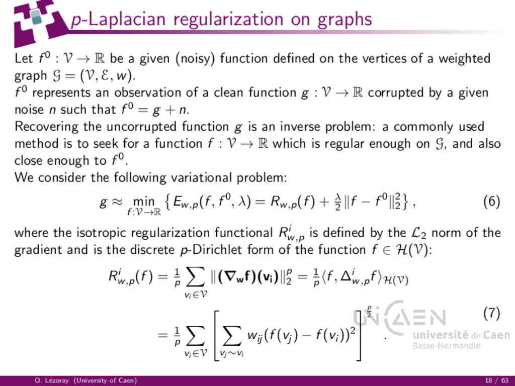
24. p-Laplacian regularization on graphs Let f 0 : V → R be a given (noisy) function defined on the vertices of a weighted graph G = (V, E, w). f 0 represents an observation of a clean function g : V → R corrupted by a given noise n such that f 0 = g + n. Recovering the uncorrupted function g is an inverse problem: a commonly used method is to seek for a function f : V → R which is regular enough on G, and also close enough to f 0. We consider the following variational problem: g ≈ min f :V→R Ew,p (f , f 0, λ) = Rw,p (f ) + λ 2 f − f 0 2 2 , (6) where the isotropic regularization functional Ri w,p is defined by the L2 norm of the gradient and is the discrete p-Dirichlet form of the function f ∈ H(V): Ri w,p (f ) = 1 p vi ∈V (∇w f)(vi ) p 2 = 1 p f , ∆i w,p f H(V) = 1 p vi ∈V   vj ∼vi wij (f (vj ) − f (vi ))2   p 2 . (7) O. L´ ezoray (University of Caen) 18 / 63
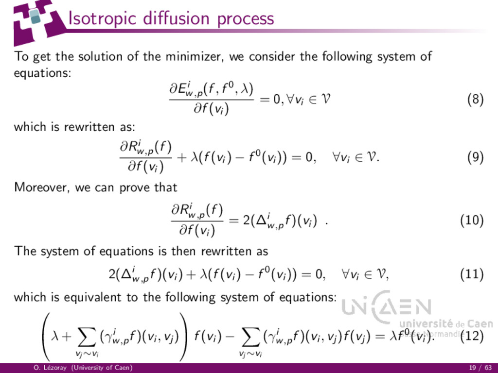
25. Isotropic diffusion process To get the solution of the minimizer, we consider the following system of equations: ∂Ei w,p (f , f 0, λ) ∂f (vi ) = 0, ∀vi ∈ V (8) which is rewritten as: ∂Ri w,p (f ) ∂f (vi ) + λ(f (vi ) − f 0(vi )) = 0, ∀vi ∈ V. (9) Moreover, we can prove that ∂Ri w,p (f ) ∂f (vi ) = 2(∆i w,p f )(vi ) . (10) The system of equations is then rewritten as 2(∆i w,p f )(vi ) + λ(f (vi ) − f 0(vi )) = 0, ∀vi ∈ V, (11) which is equivalent to the following system of equations:  λ + vj ∼vi (γi w,p f )(vi , vj )   f (vi ) − vj ∼vi (γi w,p f )(vi , vj )f (vj ) = λf 0(vi ). (12) O. L´ ezoray (University of Caen) 19 / 63
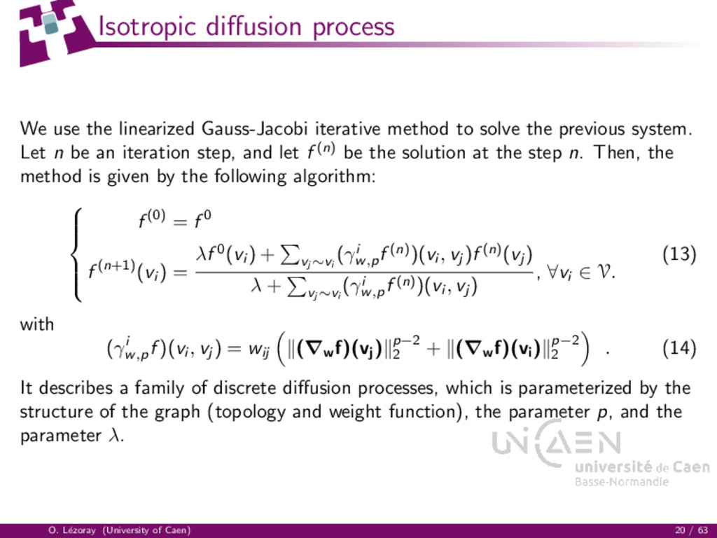
26. Isotropic diffusion process We use the linearized Gauss-Jacobi iterative method to solve the previous system. Let n be an iteration step, and let f (n) be the solution at the step n. Then, the method is given by the following algorithm:        f (0) = f 0 f (n+1)(vi ) = λf 0(vi ) + vj ∼vi (γi w,p f (n))(vi , vj )f (n)(vj ) λ + vj ∼vi (γi w,p f (n))(vi , vj ) , ∀vi ∈ V. (13) with (γi w,p f )(vi , vj ) = wij (∇w f)(vj ) p−2 2 + (∇w f)(vi ) p−2 2 . (14) It describes a family of discrete diffusion processes, which is parameterized by the structure of the graph (topology and weight function), the parameter p, and the parameter λ. O. L´ ezoray (University of Caen) 20 / 63
27. Image filtering Cytological and Histological image filtering (p = 1, λ = 10−3). O. L´ ezoray (University of Caen) 21 / 63
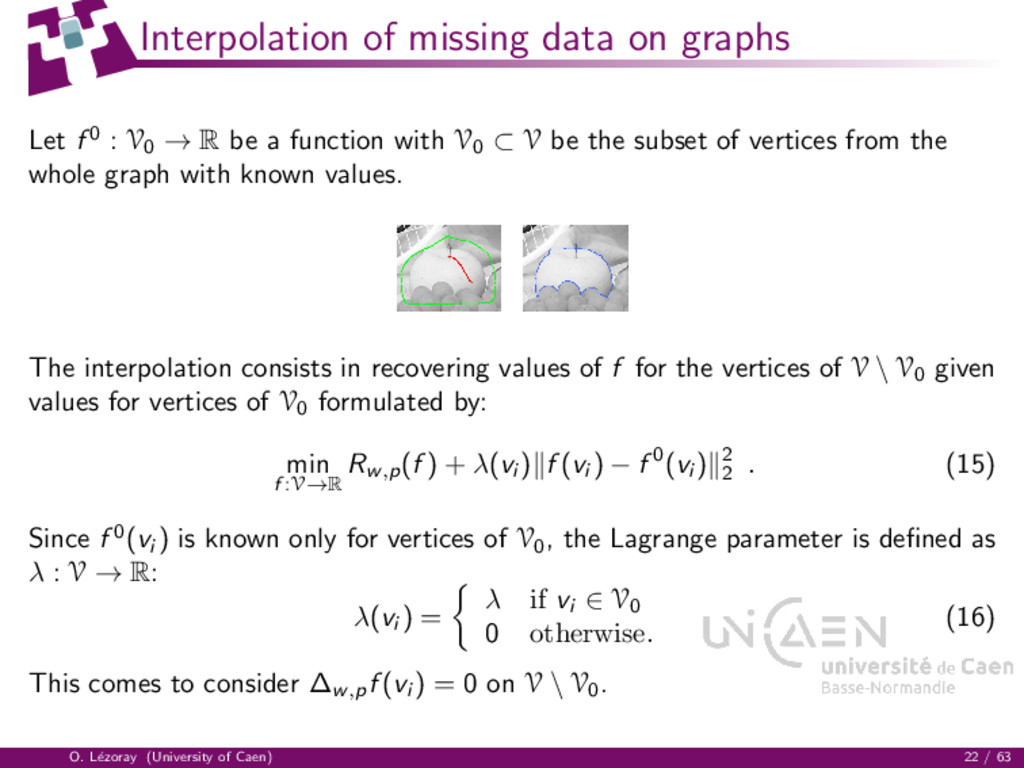
28. Interpolation of missing data on graphs Let f 0 : V0 → R be a function with V0 ⊂ V be the subset of vertices from the whole graph with known values. The interpolation consists in recovering values of f for the vertices of V \ V0 given values for vertices of V0 formulated by: min f :V→R Rw,p (f ) + λ(vi ) f (vi ) − f 0(vi ) 2 2 . (15) Since f 0(vi ) is known only for vertices of V0 , the Lagrange parameter is defined as λ : V → R: λ(vi ) = λ if vi ∈ V0 0 otherwise. (16) This comes to consider ∆w,p f (vi ) = 0 on V \ V0 . O. L´ ezoray (University of Caen) 22 / 63
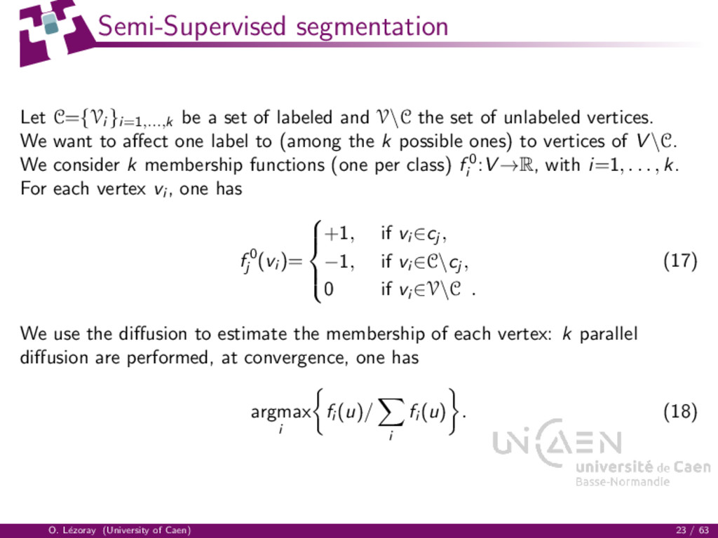
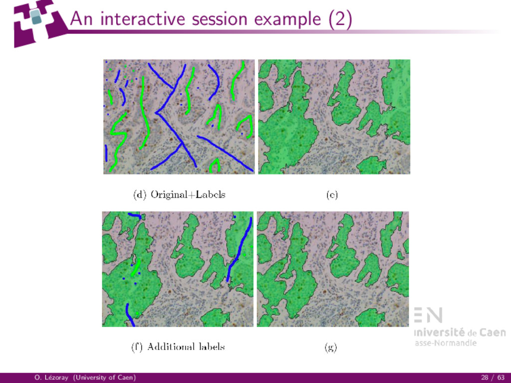
29. Semi-Supervised segmentation Let C={Vi }i=1,...,k be a set of labeled and V\C the set of unlabeled vertices. We want to affect one label to (among the k possible ones) to vertices of V \C. We consider k membership functions (one per class) f 0 i :V →R, with i=1, . . . , k. For each vertex vi , one has f 0 j (vi )=      +1, if vi ∈cj , −1, if vi ∈C\cj , 0 if vi ∈V\C . (17) We use the diffusion to estimate the membership of each vertex: k parallel diffusion are performed, at convergence, one has argmax i fi (u)/ i fi (u) . (18) O. L´ ezoray (University of Caen) 23 / 63
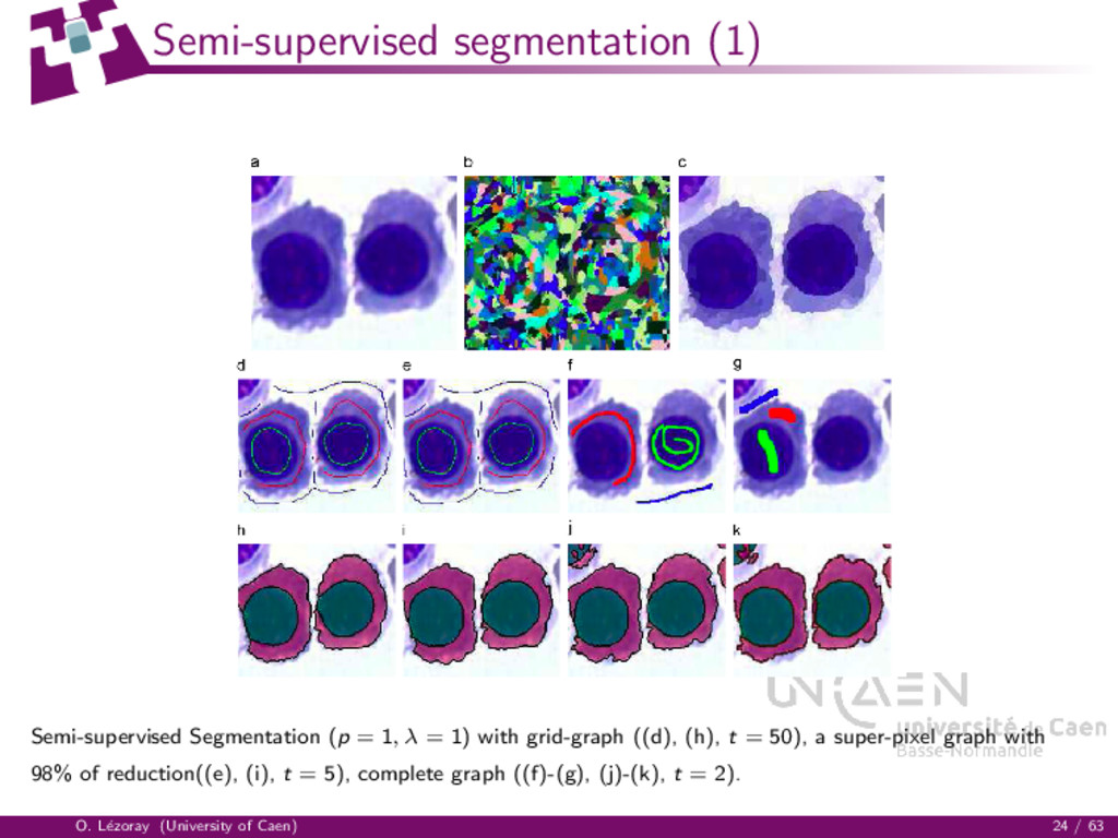
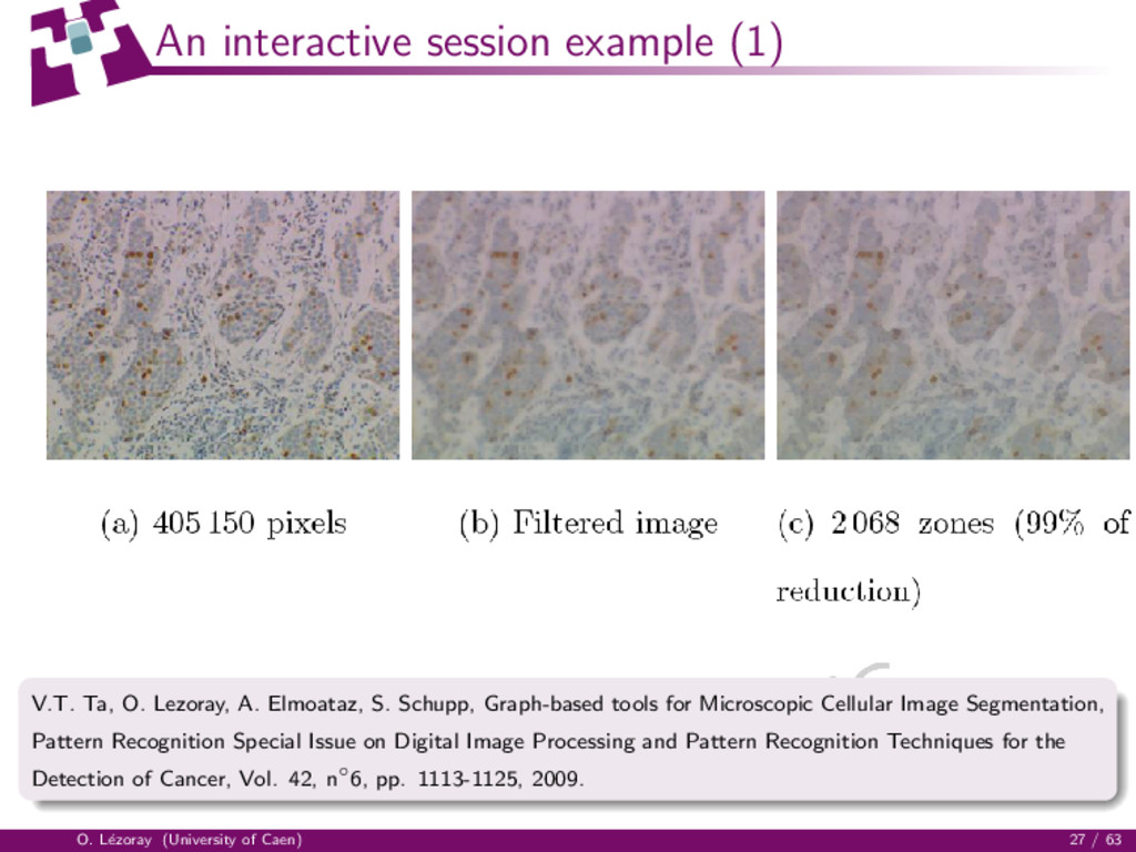
30. Semi-supervised segmentation (1) Semi-supervised Segmentation (p = 1, λ = 1) with grid-graph ((d), (h), t = 50), a super-pixel graph with 98% of reduction((e), (i), t = 5), complete graph ((f)-(g), (j)-(k), t = 2). O. L´ ezoray (University of Caen) 24 / 63
31. Semi-supervised segmentation (2) O. L´ ezoray (University of Caen) 25 / 63
32. Unsupervised segmentation O. L´ ezoray (University of Caen) 26 / 63
33. An interactive session example (1) V.T. Ta, O. Lezoray, A. Elmoataz, S. Schupp, Graph-based tools for Microscopic Cellular Image Segmentation, Pattern Recognition Special Issue on Digital Image Processing and Pattern Recognition Techniques for the Detection of Cancer, Vol. 42, n◦6, pp. 1113-1125, 2009. O. L´ ezoray (University of Caen) 27 / 63
34. An interactive session example (2) O. L´ ezoray (University of Caen) 28 / 63
35. 1 Introduction 2 Regularization on graphs 3 Multi-resolution Segmentation Methods of Breast and Equine Tendon Histological WSI Multi-resolution Segmentation Method of Breast Histological WSI Image Analysis Method of Equine Tendon Histological WSI 4 High-content screening in cytological digital slides O. L´ ezoray (University of Caen) 29 / 63
36. 1 Introduction 2 Regularization on graphs Processing graphs signals Weighted graphs Basics Operators on graphs p-Laplacian regularization on graphs 3 Multi-resolution Segmentation Methods of Breast and Equine Tendon Histological WSI Multi-resolution Segmentation Method of Breast Histological WSI Image Analysis Method of Equine Tendon Histological WSI 4 High-content screening in cytological digital slides O. L´ ezoray (University of Caen) 30 / 63
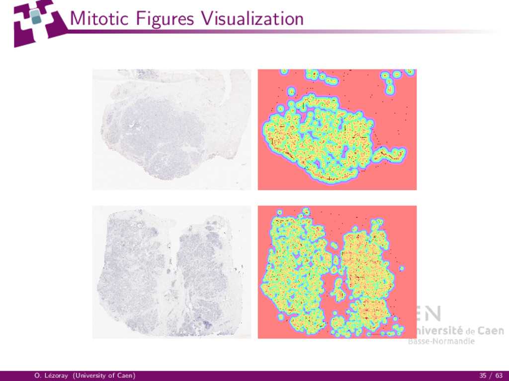
37. Background Breast Cancer Second leading cause of cancer death for women; Breast cancer grading : Elston-Ellis criterion Proliferation of mitotic figures is one of the strongest prognostic and predictive factor in breast carcinoma Our Approach on Breast Cancer Histological WSI Graph-based multi-resolution segmentation; Top-down approach that mimics pathologist interpretation process; Segmentation based on two important steps : 1 Unsupervised clustering process at each resolution level; 2 Refinement of the associated segmentation in specific areas as the resolution increases; V. Roullier, O. L´ ezoray, V.T. Ta, A. Elmoataz, Multi-resolution graph-based analysis of histopathological whole slide images: application to mitotic cell extraction and visualization, Computerized Medical Imaging and Graphics, Vol. 35, pp. 603-615, 2011. O. L´ ezoray (University of Caen) 31 / 63
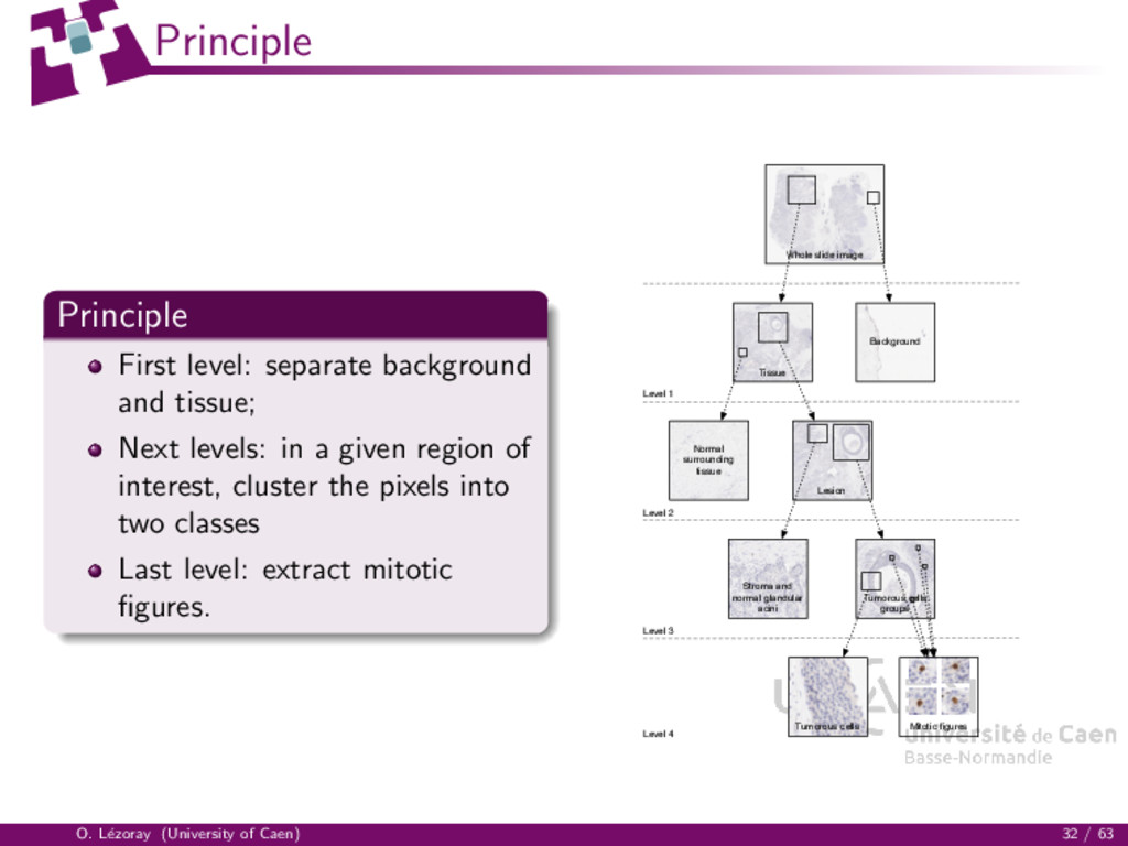
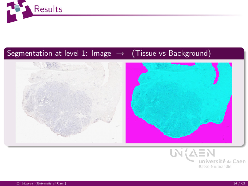
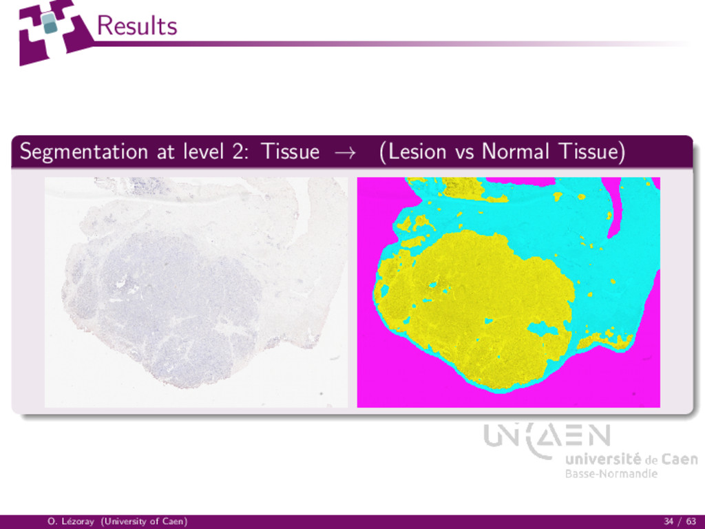
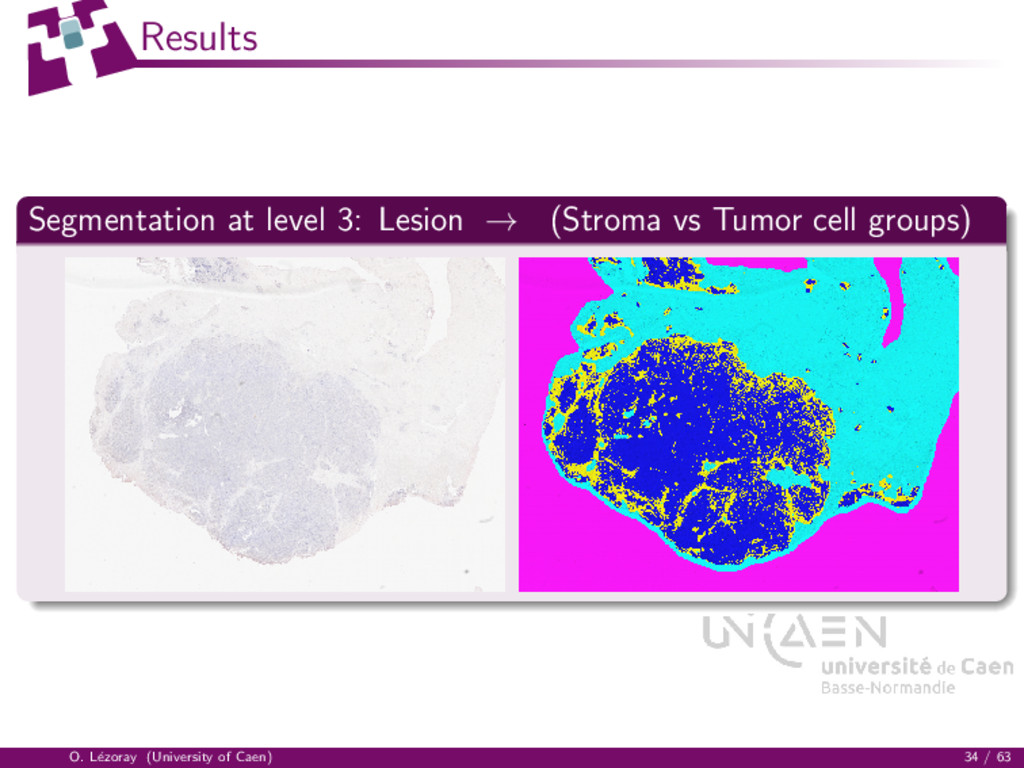
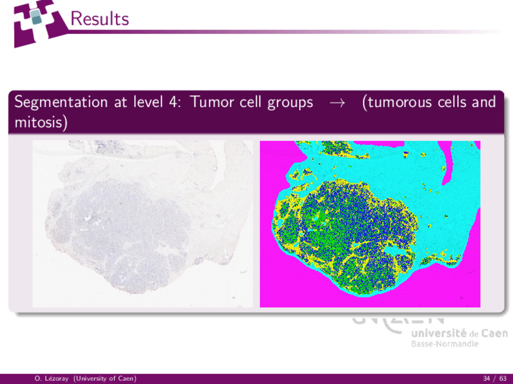
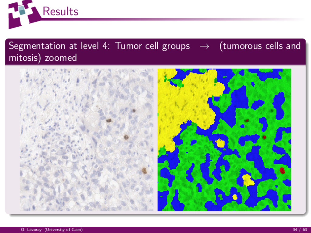
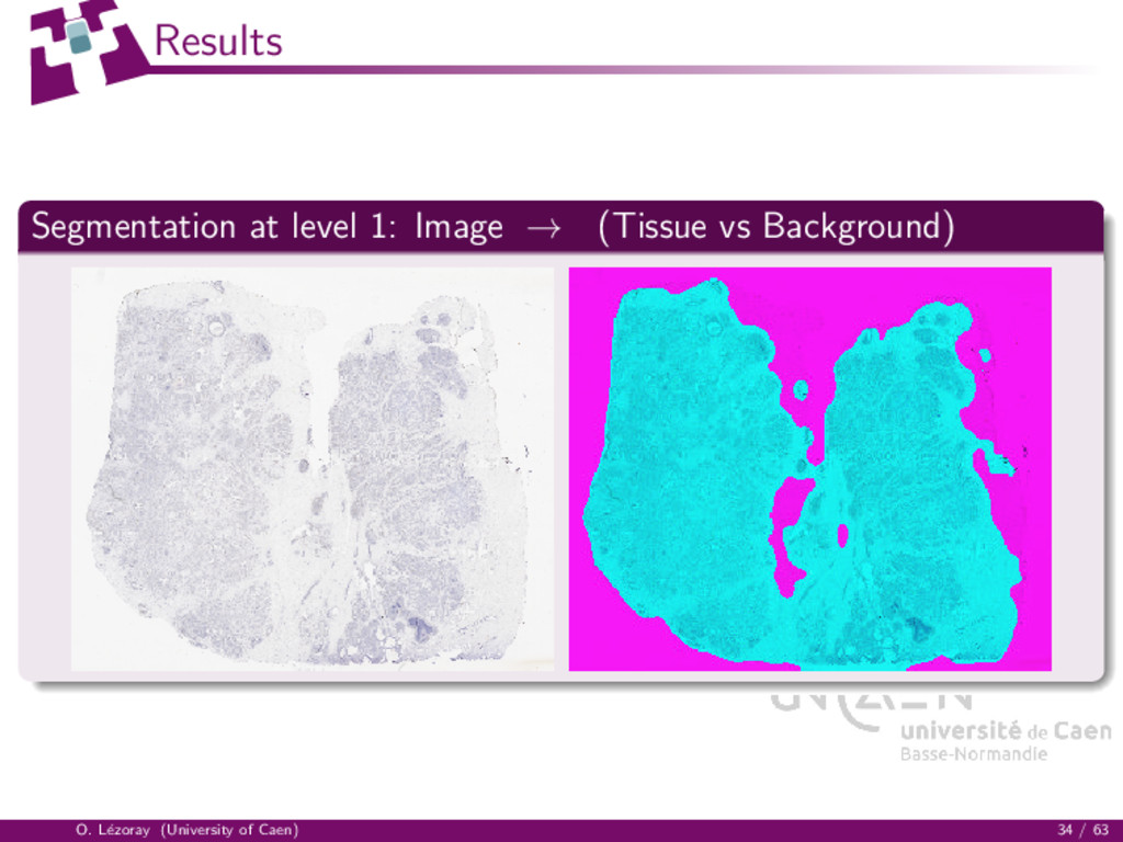
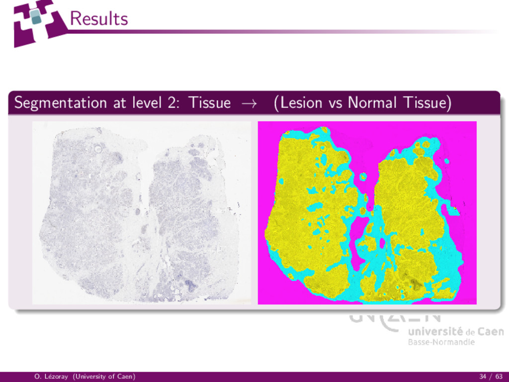
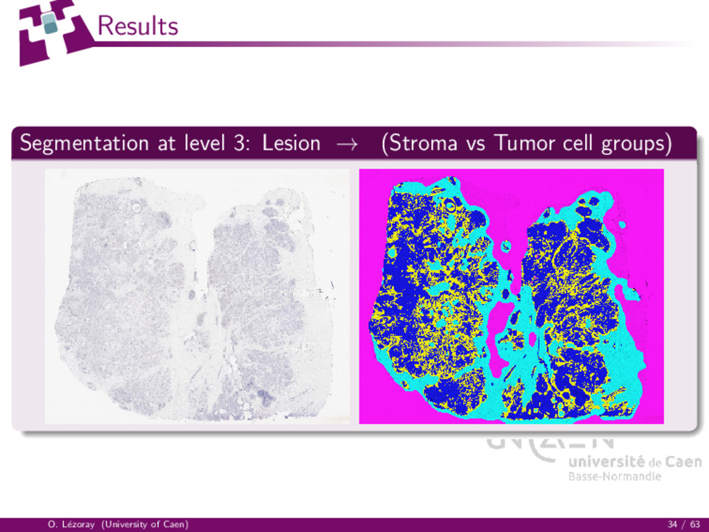
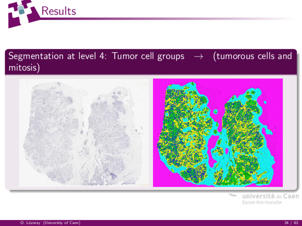
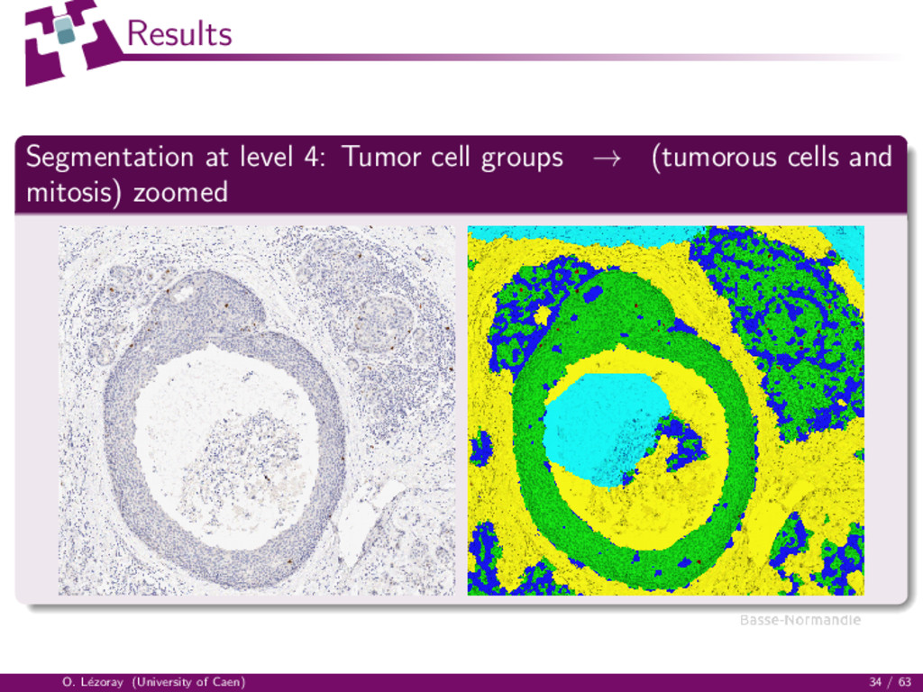
38. Principle Principle First level: separate background and tissue; Next levels: in a given region of interest, cluster the pixels into two classes Last level: extract mitotic figures. Background Whole slide image Normal surrounding tissue Tissue Stroma and normal glandular acini Lesion Tumorous cells Tumorous cells groups Mitotic figures Level 2 Level 3 Level 1 Level 4 O. L´ ezoray (University of Caen) 32 / 63
39. General Algorithm Algorithm O. L´ ezoray (University of Caen) 33 / 63
40. General Algorithm Algorithm 1 Regularization of the image tiles O. L´ ezoray (University of Caen) 33 / 63
41. General Algorithm Algorithm 1 Regularization of the image tiles 2 Unsupervised clustering (color) in 2 classes of the Histogram of the tiles O. L´ ezoray (University of Caen) 33 / 63
42. General Algorithm Algorithm 1 Regularization of the image tiles 2 Unsupervised clustering (color) in 2 classes of the Histogram of the tiles 3 Spatial refinement O. L´ ezoray (University of Caen) 33 / 63
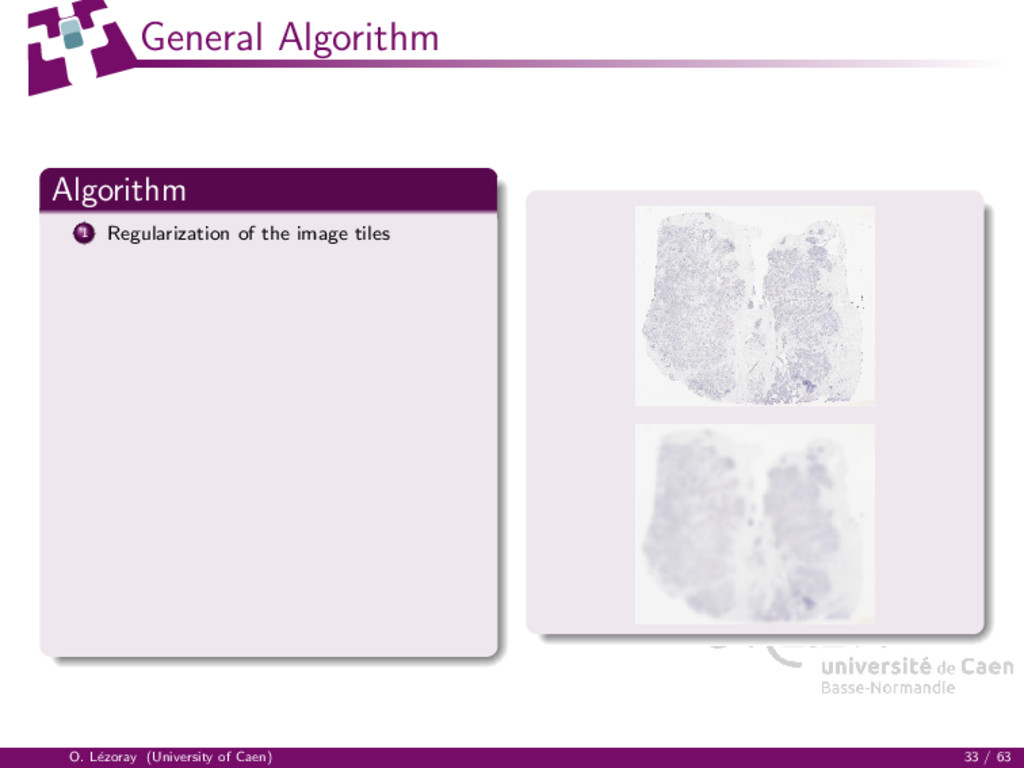
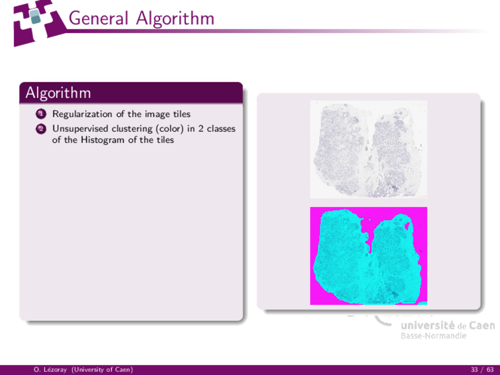
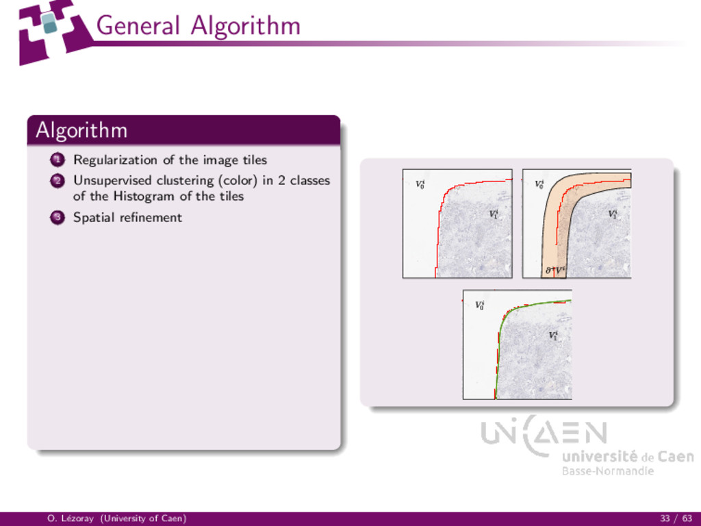
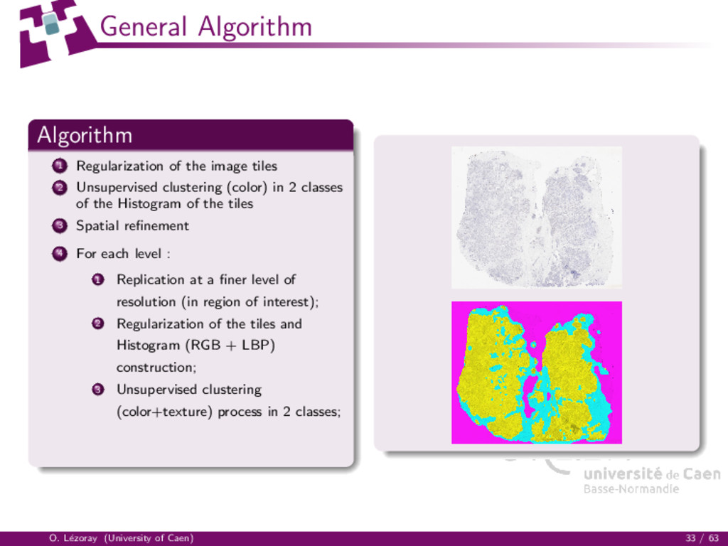
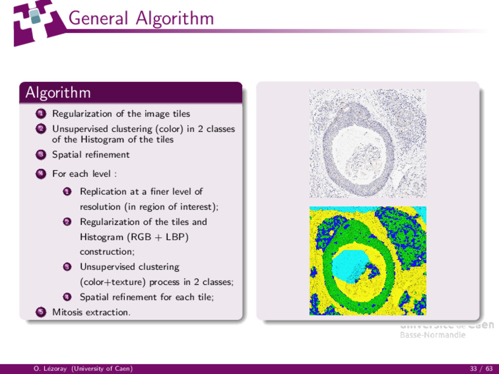
43. General Algorithm Algorithm 1 Regularization of the image tiles 2 Unsupervised clustering (color) in 2 classes of the Histogram of the tiles 3 Spatial refinement 4 For each level : O. L´ ezoray (University of Caen) 33 / 63
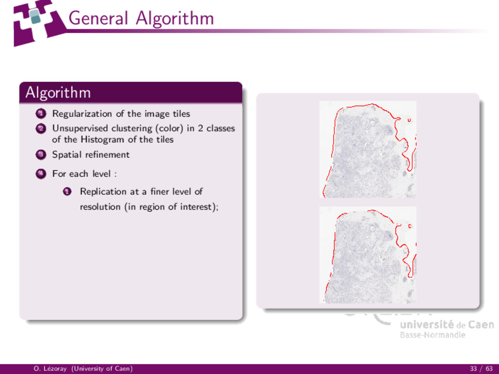
44. General Algorithm Algorithm 1 Regularization of the image tiles 2 Unsupervised clustering (color) in 2 classes of the Histogram of the tiles 3 Spatial refinement 4 For each level : 1 Replication at a finer level of resolution (in region of interest); O. L´ ezoray (University of Caen) 33 / 63
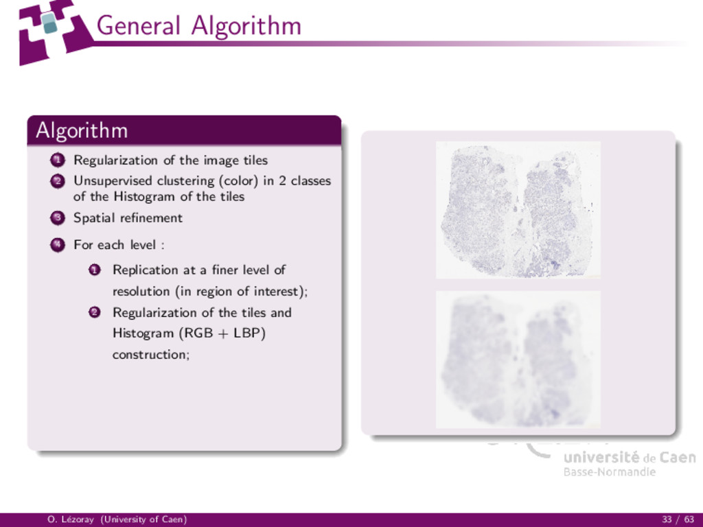
45. General Algorithm Algorithm 1 Regularization of the image tiles 2 Unsupervised clustering (color) in 2 classes of the Histogram of the tiles 3 Spatial refinement 4 For each level : 1 Replication at a finer level of resolution (in region of interest); 2 Regularization of the tiles and Histogram (RGB + LBP) construction; O. L´ ezoray (University of Caen) 33 / 63
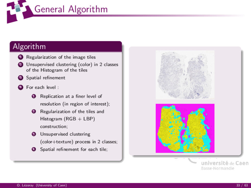
46. General Algorithm Algorithm 1 Regularization of the image tiles 2 Unsupervised clustering (color) in 2 classes of the Histogram of the tiles 3 Spatial refinement 4 For each level : 1 Replication at a finer level of resolution (in region of interest); 2 Regularization of the tiles and Histogram (RGB + LBP) construction; 3 Unsupervised clustering (color+texture) process in 2 classes; O. L´ ezoray (University of Caen) 33 / 63
47. General Algorithm Algorithm 1 Regularization of the image tiles 2 Unsupervised clustering (color) in 2 classes of the Histogram of the tiles 3 Spatial refinement 4 For each level : 1 Replication at a finer level of resolution (in region of interest); 2 Regularization of the tiles and Histogram (RGB + LBP) construction; 3 Unsupervised clustering (color+texture) process in 2 classes; 4 Spatial refinement for each tile; O. L´ ezoray (University of Caen) 33 / 63
48. General Algorithm Algorithm 1 Regularization of the image tiles 2 Unsupervised clustering (color) in 2 classes of the Histogram of the tiles 3 Spatial refinement 4 For each level : 1 Replication at a finer level of resolution (in region of interest); 2 Regularization of the tiles and Histogram (RGB + LBP) construction; 3 Unsupervised clustering (color+texture) process in 2 classes; 4 Spatial refinement for each tile; O. L´ ezoray (University of Caen) 33 / 63
49. General Algorithm Algorithm 1 Regularization of the image tiles 2 Unsupervised clustering (color) in 2 classes of the Histogram of the tiles 3 Spatial refinement 4 For each level : 1 Replication at a finer level of resolution (in region of interest); 2 Regularization of the tiles and Histogram (RGB + LBP) construction; 3 Unsupervised clustering (color+texture) process in 2 classes; 4 Spatial refinement for each tile; O. L´ ezoray (University of Caen) 33 / 63
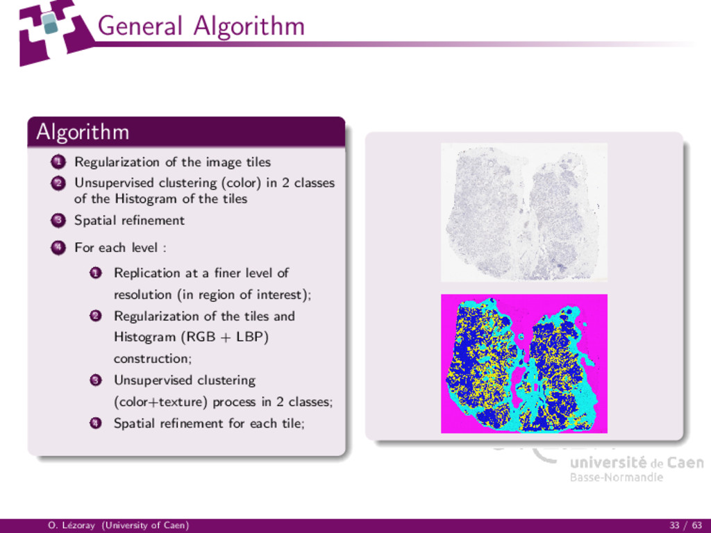
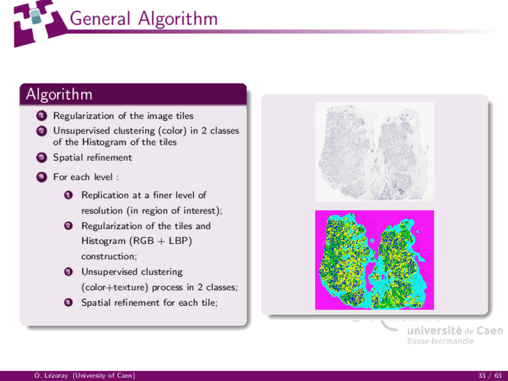
50. General Algorithm Algorithm 1 Regularization of the image tiles 2 Unsupervised clustering (color) in 2 classes of the Histogram of the tiles 3 Spatial refinement 4 For each level : 1 Replication at a finer level of resolution (in region of interest); 2 Regularization of the tiles and Histogram (RGB + LBP) construction; 3 Unsupervised clustering (color+texture) process in 2 classes; 4 Spatial refinement for each tile; 5 Mitosis extraction. O. L´ ezoray (University of Caen) 33 / 63
51. Results Segmentation at level 1: Image → (Tissue vs Background) O. L´ ezoray (University of Caen) 34 / 63
52. Results Segmentation at level 2: Tissue → (Lesion vs Normal Tissue) O. L´ ezoray (University of Caen) 34 / 63
53. Results Segmentation at level 3: Lesion → (Stroma vs Tumor cell groups) O. L´ ezoray (University of Caen) 34 / 63
54. Results Segmentation at level 4: Tumor cell groups → (tumorous cells and mitosis) O. L´ ezoray (University of Caen) 34 / 63
55. Results Segmentation at level 4: Tumor cell groups → (tumorous cells and mitosis) zoomed O. L´ ezoray (University of Caen) 34 / 63
56. Results Segmentation at level 1: Image → (Tissue vs Background) O. L´ ezoray (University of Caen) 34 / 63
57. Results Segmentation at level 2: Tissue → (Lesion vs Normal Tissue) O. L´ ezoray (University of Caen) 34 / 63
58. Results Segmentation at level 3: Lesion → (Stroma vs Tumor cell groups) O. L´ ezoray (University of Caen) 34 / 63
59. Results Segmentation at level 4: Tumor cell groups → (tumorous cells and mitosis) O. L´ ezoray (University of Caen) 34 / 63
60. Results Segmentation at level 4: Tumor cell groups → (tumorous cells and mitosis) zoomed O. L´ ezoray (University of Caen) 34 / 63
61. Mitotic Figures Visualization O. L´ ezoray (University of Caen) 35 / 63
62. 1 Introduction 2 Regularization on graphs Processing graphs signals Weighted graphs Basics Operators on graphs p-Laplacian regularization on graphs 3 Multi-resolution Segmentation Methods of Breast and Equine Tendon Histological WSI Multi-resolution Segmentation Method of Breast Histological WSI Image Analysis Method of Equine Tendon Histological WSI 4 High-content screening in cytological digital slides O. L´ ezoray (University of Caen) 36 / 63
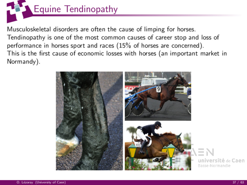
63. Equine Tendinopathy Musculoskeletal disorders are often the cause of limping for horses. Tendinopathy is one of the most common causes of career stop and loss of performance in horses sport and races (15% of horses are concerned). This is the first cause of economic losses with horses (an important market in Normandy). O. L´ ezoray (University of Caen) 37 / 63
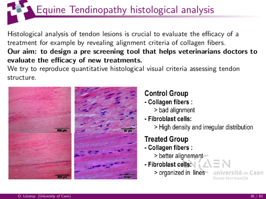
64. Equine Tendinopathy histological analysis Histological analysis of tendon lesions is crucial to evaluate the efficacy of a treatment for example by revealing alignment criteria of collagen fibers. Our aim: to design a pre screening tool that helps veterinarians doctors to evaluate the efficacy of new treatments. We try to reproduce quantitative histological visual criteria assessing tendon structure. O. L´ ezoray (University of Caen) 38 / 63
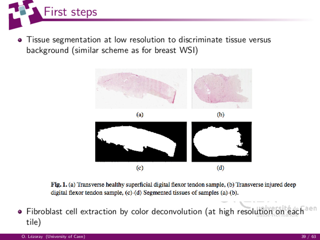
65. First steps Tissue segmentation at low resolution to discriminate tissue versus background (similar scheme as for breast WSI) Fibroblast cell extraction by color deconvolution (at high resolution on each tile) O. L´ ezoray (University of Caen) 39 / 63
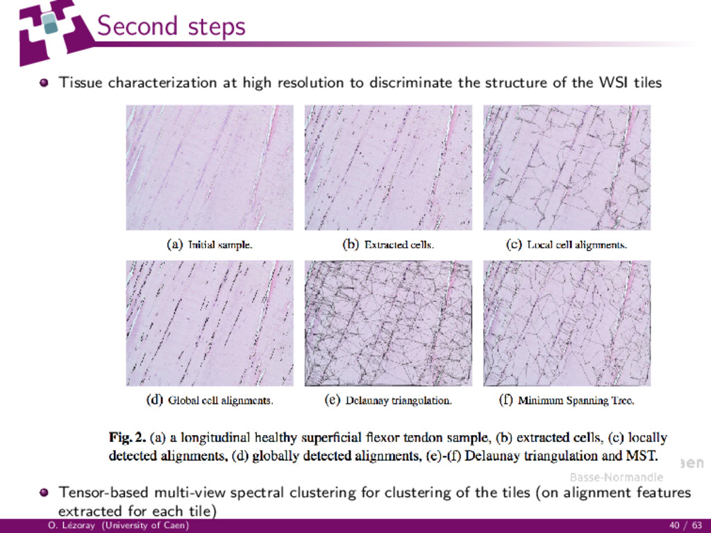
66. Second steps Tissue characterization at high resolution to discriminate the structure of the WSI tiles Tensor-based multi-view spectral clustering for clustering of the tiles (on alignment features extracted for each tile) O. L´ ezoray (University of Caen) 40 / 63
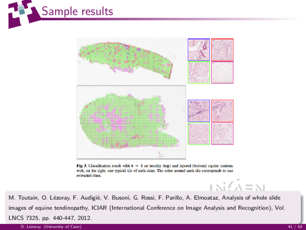
67. Sample results M. Toutain, O. L´ ezoray, F. Audigi´ e, V. Busoni, G. Rossi, F. Parillo, A. Elmoataz, Analysis of whole slide images of equine tendinopathy, ICIAR (International Conference on Image Analysis and Recognition), Vol. LNCS 7325, pp. 440-447, 2012. O. L´ ezoray (University of Caen) 41 / 63
68. 1 Introduction 2 Regularization on graphs 3 Multi-resolution Segmentation Methods of Breast and Equine Tendon Histological WSI 4 High-content screening in cytological digital slides O. L´ ezoray (University of Caen) 42 / 63
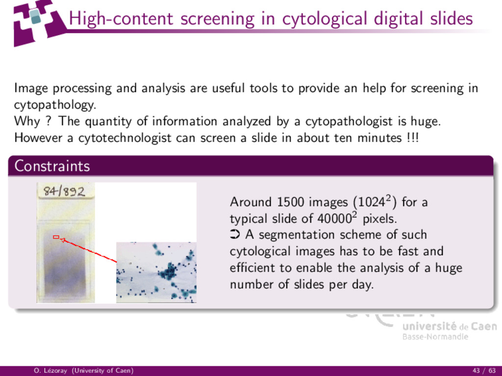
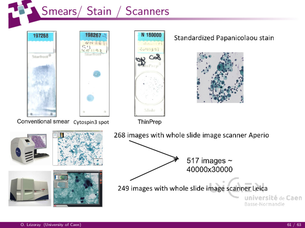
69. High-content screening in cytological digital slides Image processing and analysis are useful tools to provide an help for screening in cytopathology. Why ? The quantity of information analyzed by a cytopathologist is huge. However a cytotechnologist can screen a slide in about ten minutes !!! Constraints Around 1500 images (10242) for a typical slide of 400002 pixels. · A segmentation scheme of such cytological images has to be fast and efficient to enable the analysis of a huge number of slides per day. O. L´ ezoray (University of Caen) 43 / 63
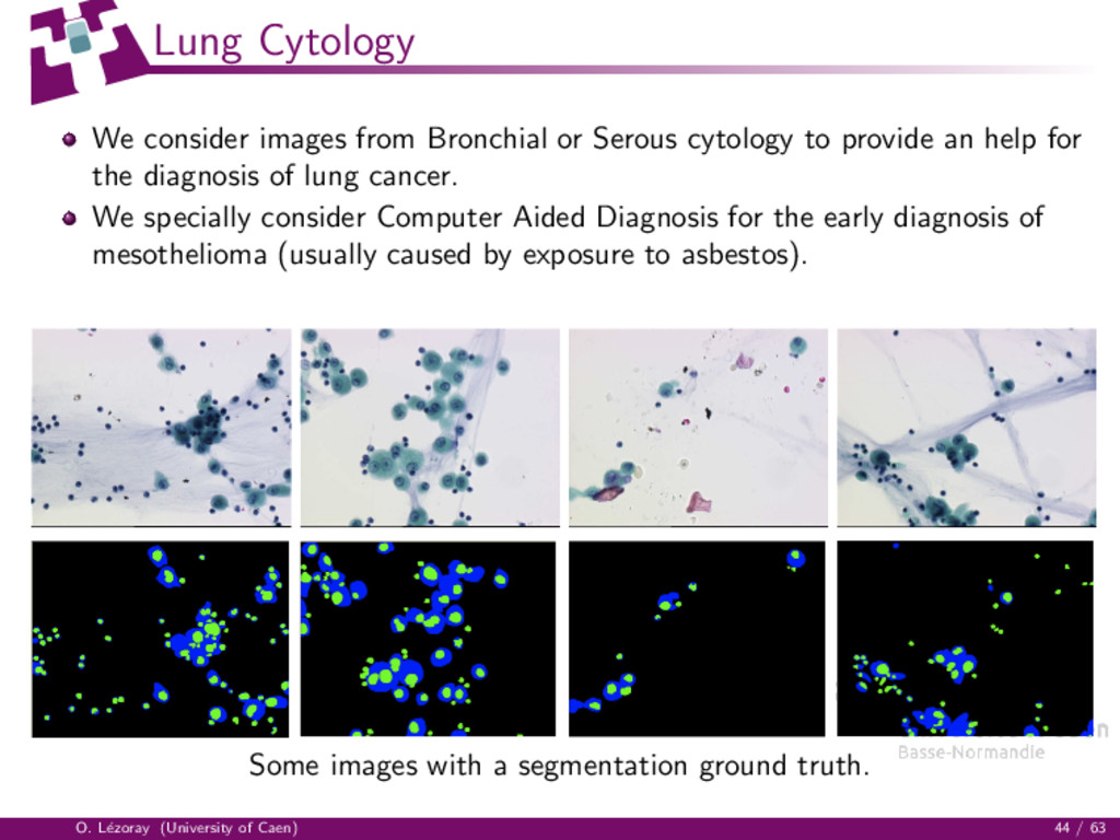
70. Lung Cytology We consider images from Bronchial or Serous cytology to provide an help for the diagnosis of lung cancer. We specially consider Computer Aided Diagnosis for the early diagnosis of mesothelioma (usually caused by exposure to asbestos). Some images with a segmentation ground truth. O. L´ ezoray (University of Caen) 44 / 63
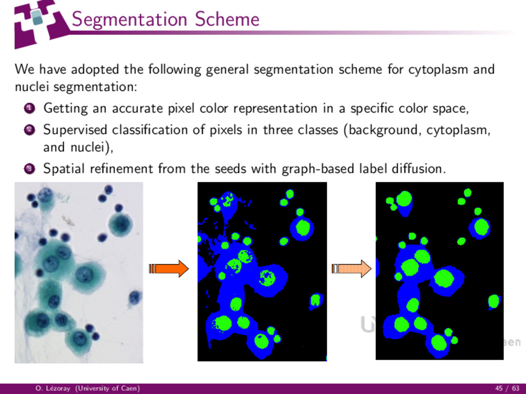
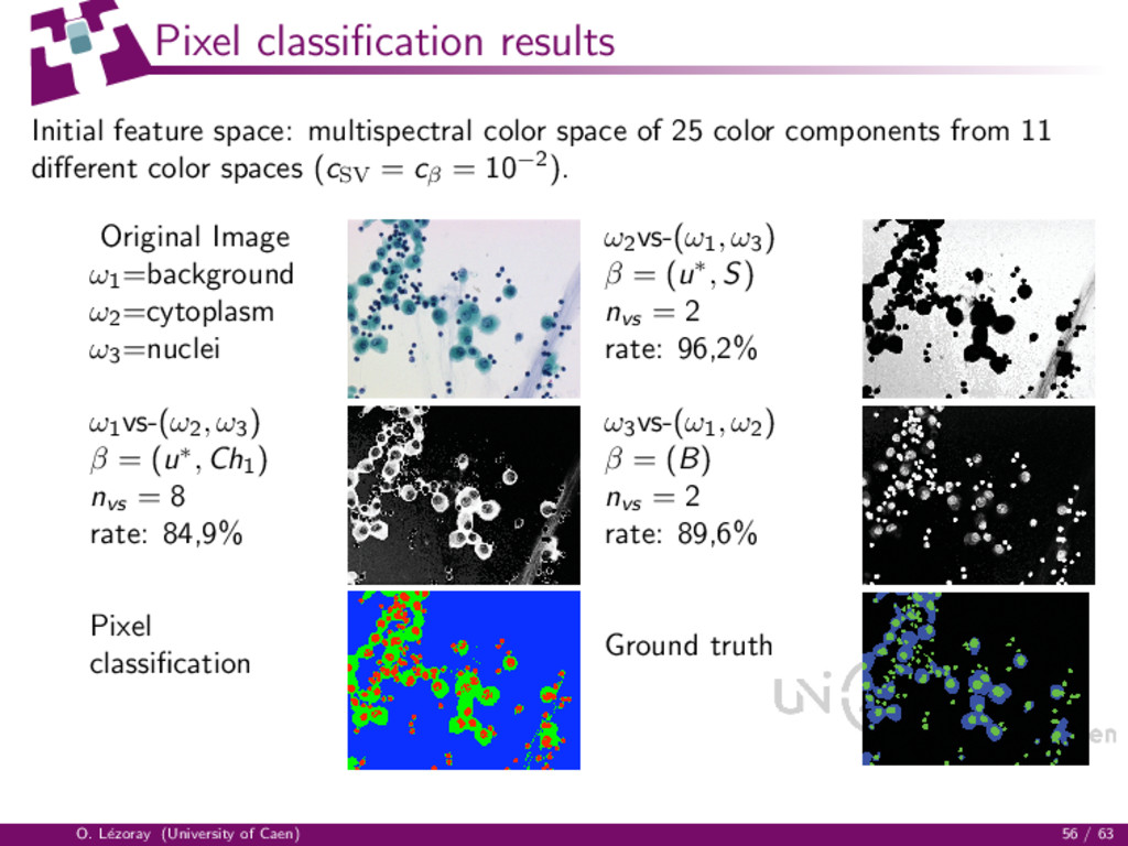
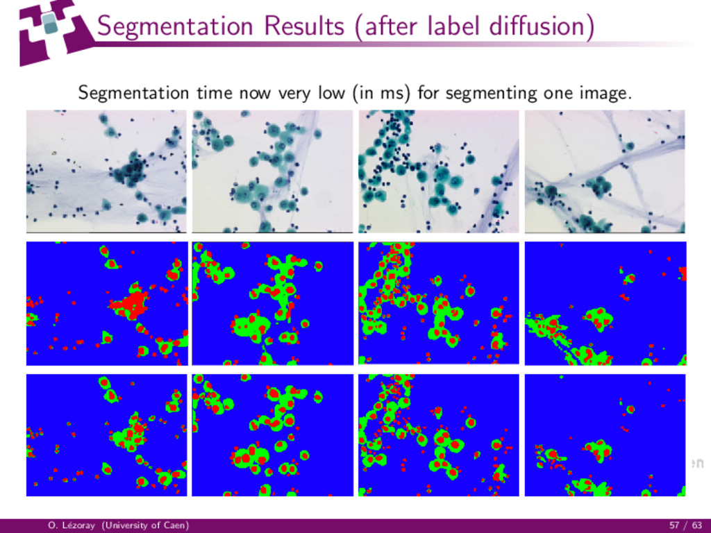
71. Segmentation Scheme We have adopted the following general segmentation scheme for cytoplasm and nuclei segmentation: 1 Getting an accurate pixel color representation in a specific color space, 2 Supervised classification of pixels in three classes (background, cytoplasm, and nuclei), 3 Spatial refinement from the seeds with graph-based label diffusion. O. L´ ezoray (University of Caen) 45 / 63
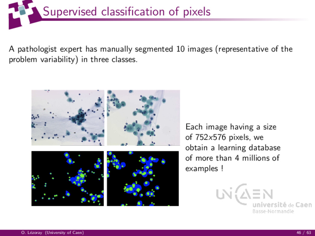
72. Supervised classification of pixels A pathologist expert has manually segmented 10 images (representative of the problem variability) in three classes. Each image having a size of 752x576 pixels, we obtain a learning database of more than 4 millions of examples ! O. L´ ezoray (University of Caen) 46 / 63
73. Sample results of supervised pixel classification Cytoplasm (top) and nuclei (bottom) classification rates. O. L´ ezoray (University of Caen) 47 / 63
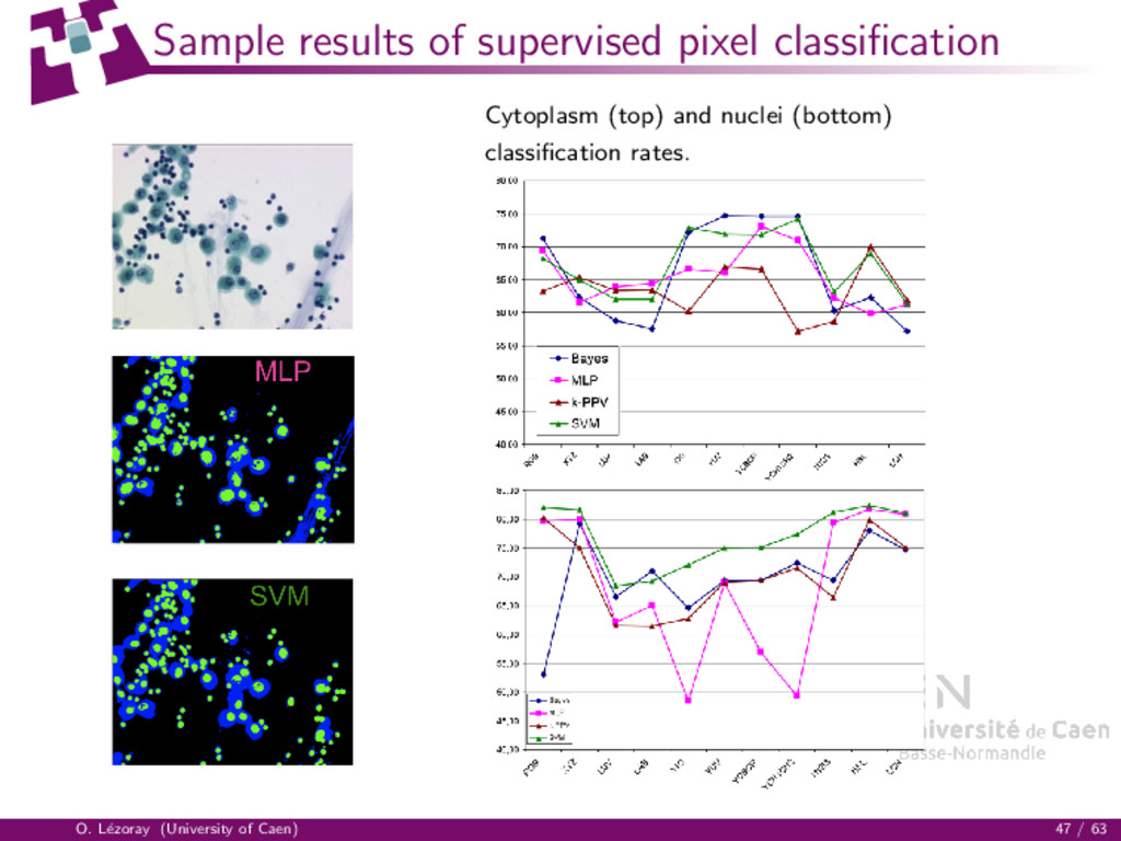
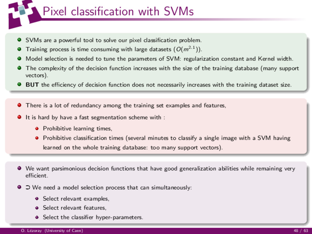
74. Pixel classification with SVMs SVMs are a powerful tool to solve our pixel classification problem. Training process is time consuming with large datasets (O(m2.1)). Model selection is needed to tune the parameters of SVM: regularization constant and Kernel width. The complexity of the decision function increases with the size of the training database (many support vectors). BUT the efficiency of decision function does not necessarily increases with the training dataset size. There is a lot of redundancy among the training set examples and features, It is hard by have a fast segmentation scheme with : Prohibitive learning times, Prohibitive classification times (several minutes to classify a single image with a SVM having learned on the whole training database: too many support vectors). We want parsimonious decision functions that have good generalization abilities while remaining very efficient. · We need a model selection process that can simultaneously: Select relevant examples, Select relevant features, Select the classifier hyper-parameters. O. L´ ezoray (University of Caen) 48 / 63
75. Selecting relevant examples (1) To reduce the size of the training database, we use an algorithm for data quantization (LBG). O. L´ ezoray (University of Caen) 49 / 63
76. Selecting relevant examples (2) · The separating hyperplane found with SVMs on the quantized database is a good approximation of the one found on the original database. O. L´ ezoray (University of Caen) 50 / 63
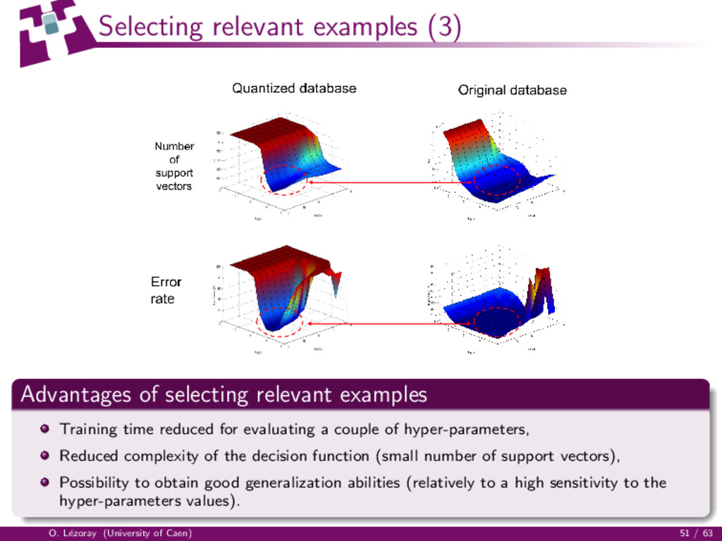
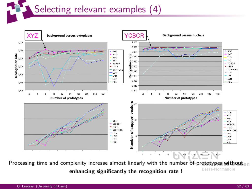
77. Selecting relevant examples (3) Advantages of selecting relevant examples Training time reduced for evaluating a couple of hyper-parameters, Reduced complexity of the decision function (small number of support vectors), Possibility to obtain good generalization abilities (relatively to a high sensitivity to the hyper-parameters values). O. L´ ezoray (University of Caen) 51 / 63
78. Selecting relevant examples (4) Processing time and complexity increase almost linearly with the number of prototypes without enhancing significantly the recognition rate ! O. L´ ezoray (University of Caen) 52 / 63
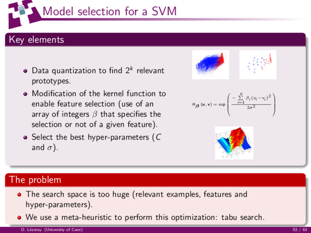
79. Model selection for a SVM Key elements Data quantization to find 2k relevant prototypes. Modification of the kernel function to enable feature selection (use of an array of integers β that specifies the selection or not of a given feature). Select the best hyper-parameters (C and σ). Kβ (u, v) = exp      − n i=1 βi ui −vi 2 2σ2      The problem The search space is too huge (relevant examples, features and hyper-parameters). We use a meta-heuristic to perform this optimization: tabu search. O. L´ ezoray (University of Caen) 53 / 63
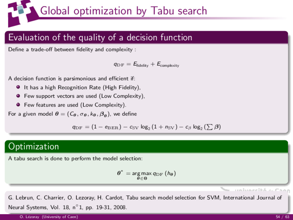
80. Global optimization by Tabu search Evaluation of the quality of a decision function Define a trade-off between fidelity and complexity : qDF = Efidelity + Ecomplexity A decision function is parsimonious and efficient if: It has a high Recognition Rate (High Fidelity), Few support vectors are used (Low Complexity), Few features are used (Low Complexity). For a given model θ = (Cθ, σθ, kθ, βθ ), we define qDF = (1 − eBER) − cSV log2 (1 + nSV) − cβ log2 ( β) Optimization A tabu search is done to perform the model selection: θ∗ = arg max θ∈Θ qDF (hθ) G. Lebrun, C. Charrier, O. Lezoray, H. Cardot, Tabu search model selection for SVM, International Journal of Neural Systems, Vol. 18, n◦1, pp. 19-31, 2008. O. L´ ezoray (University of Caen) 54 / 63
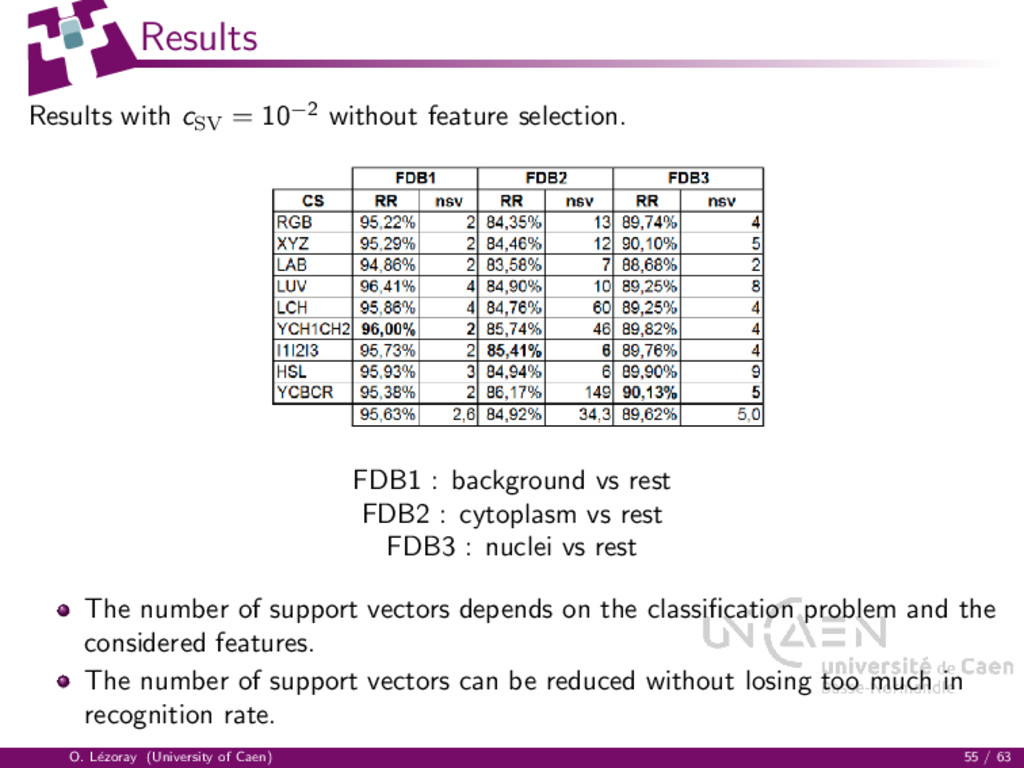
81. Results Results with cSV = 10−2 without feature selection. FDB1 : background vs rest FDB2 : cytoplasm vs rest FDB3 : nuclei vs rest The number of support vectors depends on the classification problem and the considered features. The number of support vectors can be reduced without losing too much in recognition rate. O. L´ ezoray (University of Caen) 55 / 63
82. Pixel classification results Initial feature space: multispectral color space of 25 color components from 11 different color spaces (cSV = cβ = 10−2). Original Image ω1 =background ω2 =cytoplasm ω3 =nuclei ω2 vs-(ω1, ω3 ) β = (u∗, S) nvs = 2 rate: 96,2% ω1 vs-(ω2, ω3 ) β = (u∗, Ch1 ) nvs = 8 rate: 84,9% ω3 vs-(ω1, ω2 ) β = (B) nvs = 2 rate: 89,6% Pixel classification Ground truth O. L´ ezoray (University of Caen) 56 / 63
83. Segmentation Results (after label diffusion) Segmentation time now very low (in ms) for segmenting one image. O. L´ ezoray (University of Caen) 57 / 63
84. Segmentation Results O. L´ ezoray (University of Caen) 58 / 63
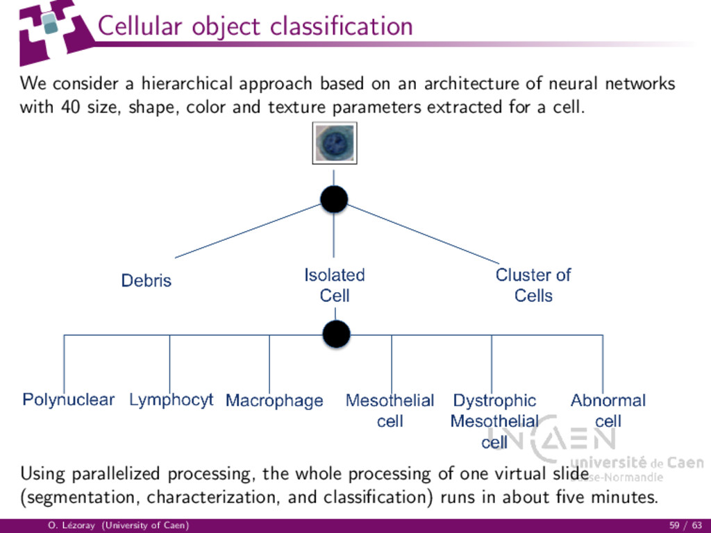
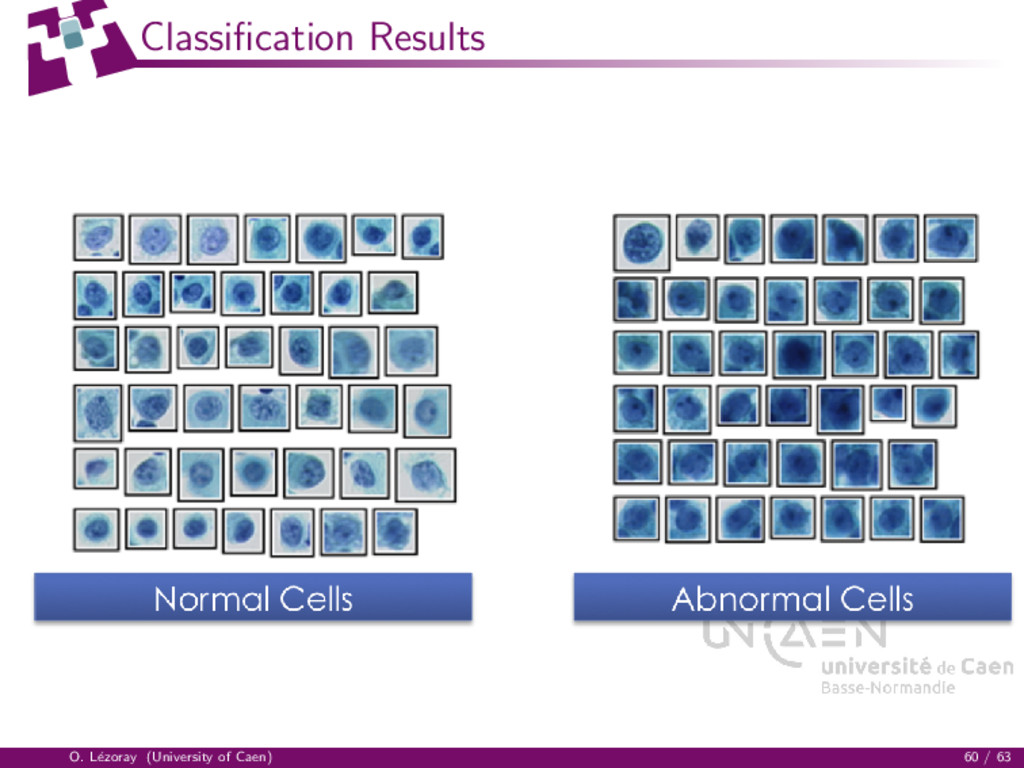
85. Cellular object classification We consider a hierarchical approach based on an architecture of neural networks with 40 size, shape, color and texture parameters extracted for a cell. Using parallelized processing, the whole processing of one virtual slide (segmentation, characterization, and classification) runs in about five minutes. O. L´ ezoray (University of Caen) 59 / 63
86. Classification Results O. L´ ezoray (University of Caen) 60 / 63
87. Smears/ Stain / Scanners O. L´ ezoray (University of Caen) 61 / 63
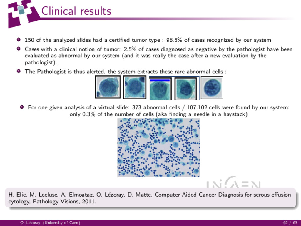
88. Clinical results 150 of the analyzed slides had a certified tumor type : 98.5% of cases recognized by our system Cases with a clinical notion of tumor: 2.5% of cases diagnosed as negative by the pathologist have been evaluated as abnormal by our system (and it was really the case after a new evaluation by the pathologist). The Pathologist is thus alerted, the system extracts these rare abnormal cells : For one given analysis of a virtual slide: 373 abnormal cells / 107.102 cells were found by our system: only 0.3% of the number of cells (aka finding a needle in a haystack) H. Elie, M. Lecluse, A. Elmoataz, O. L´ ezoray, D. Matte, Computer Aided Cancer Diagnosis for serous effusion cytology, Pathology Visions, 2011. O. L´ ezoray (University of Caen) 62 / 63
89. Thanks for your attention. Publications available at : http://lezoray.users.greyc.fr O. L´ ezoray (University of Caen) 63 / 63