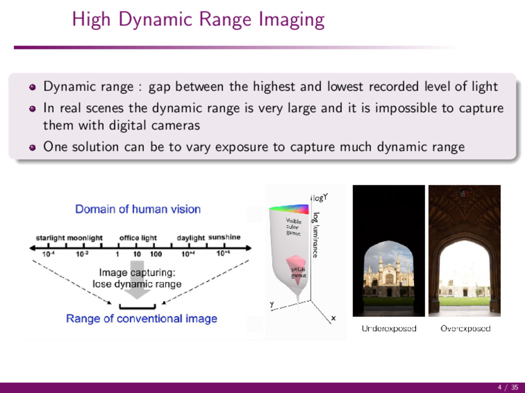
highest and lowest recorded level of light In real scenes the dynamic range is very large and it is impossible to capture them with digital cameras One solution can be to vary exposure to capture much dynamic range 4 / 35
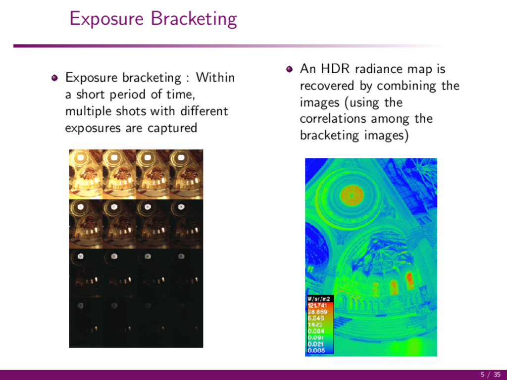
time, multiple shots with different exposures are captured An HDR radiance map is recovered by combining the images (using the correlations among the bracketing images) 5 / 35
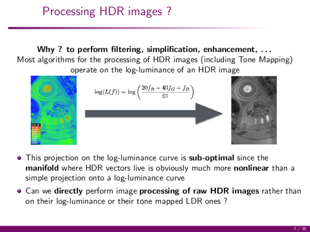
enhancement, . . . Most algorithms for the processing of HDR images (including Tone Mapping) operate on the log-luminance of an HDR image This projection on the log-luminance curve is sub-optimal since the manifold where HDR vectors live is obviously much more nonlinear than a simple projection onto a log-luminance curve Can we directly perform image processing of raw HDR images rather than on their log-luminance or their tone mapped LDR ones ? 7 / 35
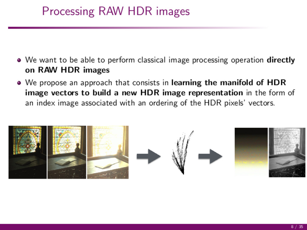
perform classical image processing operation directly on RAW HDR images We propose an approach that consists in learning the manifold of HDR image vectors to build a new HDR image representation in the form of an index image associated with an ordering of the HDR pixels’ vectors. 8 / 35
standard that associates three floating point values to pixels (RGB values of radiance). An HDR image is represented by the mapping f : Ω ⊂ Z2 → T ⊂ R3 where T is a non-empty set of image multivariate HDR vectors. To each pixel pi ∈ Ω of an image is associated a vector vi = f (pi ). The set T = {v1, · · · , vm} denotes all the HDR vectors associated to all pixels in the image, and is of size m. T [i] = vi will denote the i-th element of a set. 11 / 35
HDR image representation in the form of an index image associated with an ordering of the HDR pixels’ vectors T of an image. Ordering all the values of the set T can be done with the use of an ordering relation within HDR vectors. This amounts to dispose of a complete lattice (T , ≤) but there is no universal order for vectorial data The framework of h-orderings can be considered for that : construct a surjective mapping h from T to L where L is a complete lattice equipped with the conditional total ordering h : T → L and v → h(v), ∀(vi , vj ) ∈ T × T vi ≤h vj ⇔ h(vi ) ≤ h(vj ) . ≤h will denote such an h-ordering 12 / 35
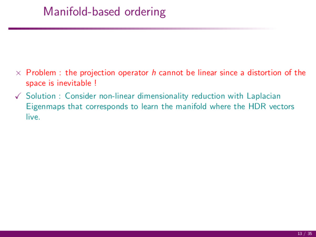
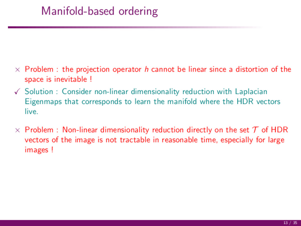
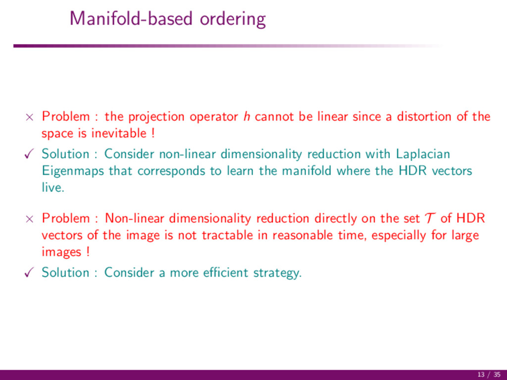
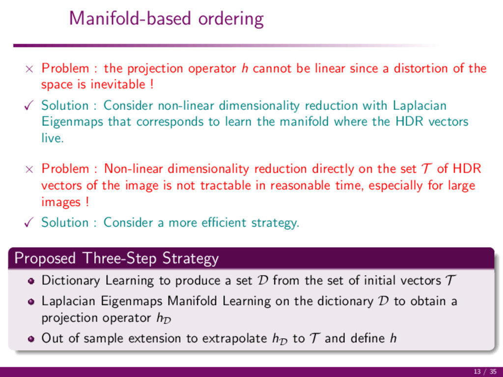
be linear since a distortion of the space is inevitable ! Solution : Consider non-linear dimensionality reduction with Laplacian Eigenmaps that corresponds to learn the manifold where the HDR vectors live. 13 / 35
be linear since a distortion of the space is inevitable ! Solution : Consider non-linear dimensionality reduction with Laplacian Eigenmaps that corresponds to learn the manifold where the HDR vectors live. × Problem : Non-linear dimensionality reduction directly on the set T of HDR vectors of the image is not tractable in reasonable time, especially for large images ! 13 / 35
be linear since a distortion of the space is inevitable ! Solution : Consider non-linear dimensionality reduction with Laplacian Eigenmaps that corresponds to learn the manifold where the HDR vectors live. × Problem : Non-linear dimensionality reduction directly on the set T of HDR vectors of the image is not tractable in reasonable time, especially for large images ! Solution : Consider a more efficient strategy. 13 / 35
be linear since a distortion of the space is inevitable ! Solution : Consider non-linear dimensionality reduction with Laplacian Eigenmaps that corresponds to learn the manifold where the HDR vectors live. × Problem : Non-linear dimensionality reduction directly on the set T of HDR vectors of the image is not tractable in reasonable time, especially for large images ! Solution : Consider a more efficient strategy. Proposed Three-Step Strategy Dictionary Learning to produce a set D from the set of initial vectors T Laplacian Eigenmaps Manifold Learning on the dictionary D to obtain a projection operator hD Out of sample extension to extrapolate hD to T and define h 13 / 35
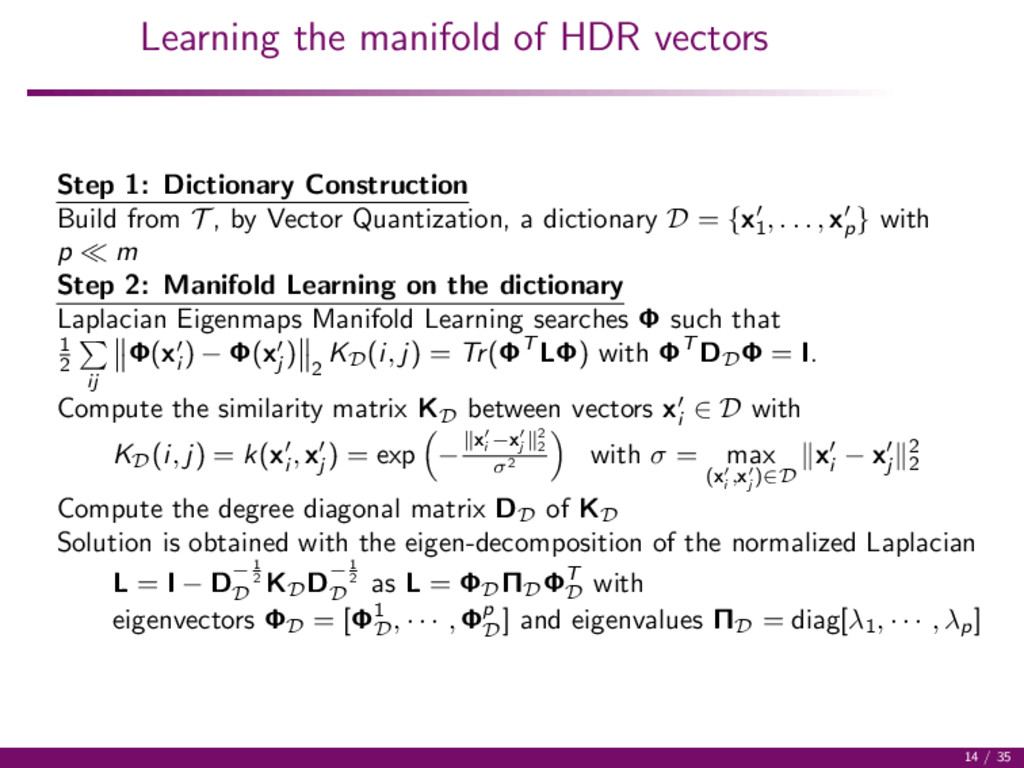
Build from T , by Vector Quantization, a dictionary D = {x1 , . . . , xp } with p m Step 2: Manifold Learning on the dictionary Laplacian Eigenmaps Manifold Learning searches Φ such that 1 2 ij Φ(xi ) − Φ(xj ) 2 KD (i, j) = Tr(ΦT LΦ) with ΦT DD Φ = I. Compute the similarity matrix KD between vectors xi ∈ D with KD (i, j) = k(xi , xj ) = exp − xi −xj 2 2 σ2 with σ = max (x i ,x j )∈D xi − xj 2 2 Compute the degree diagonal matrix DD of KD Solution is obtained with the eigen-decomposition of the normalized Laplacian L = I − D− 1 2 D KD D− 1 2 D as L = ΦD ΠD ΦT D with eigenvectors ΦD = [Φ1 D , · · · , Φp D ] and eigenvalues ΠD = diag[λ1, · · · , λp ] 14 / 35
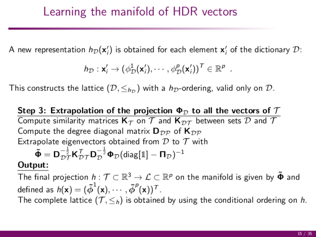
(xi ) is obtained for each element xi of the dictionary D: hD : xi → (φ1 D (xi ), · · · , φp D (xi ))T ∈ Rp . This constructs the lattice (D, ≤hD ) with a hD -ordering, valid only on D. Step 3: Extrapolation of the projection ΦD to all the vectors of T Compute similarity matrices KT on T and KDT between sets D and T Compute the degree diagonal matrix DDP of KDP Extrapolate eigenvectors obtained from D to T with ˜ Φ = D− 1 2 DT KT DT D− 1 2 D ΦD (diag[1] − ΠD )−1 Output: The final projection h : T ⊂ R3 → L ⊂ Rp on the manifold is given by ˜ Φ and defined as h(x) = ( ˜ φ1 (x), · · · , ˜ φp (x))T . The complete lattice (T , ≤h ) is obtained by using the conditional ordering on h. 15 / 35
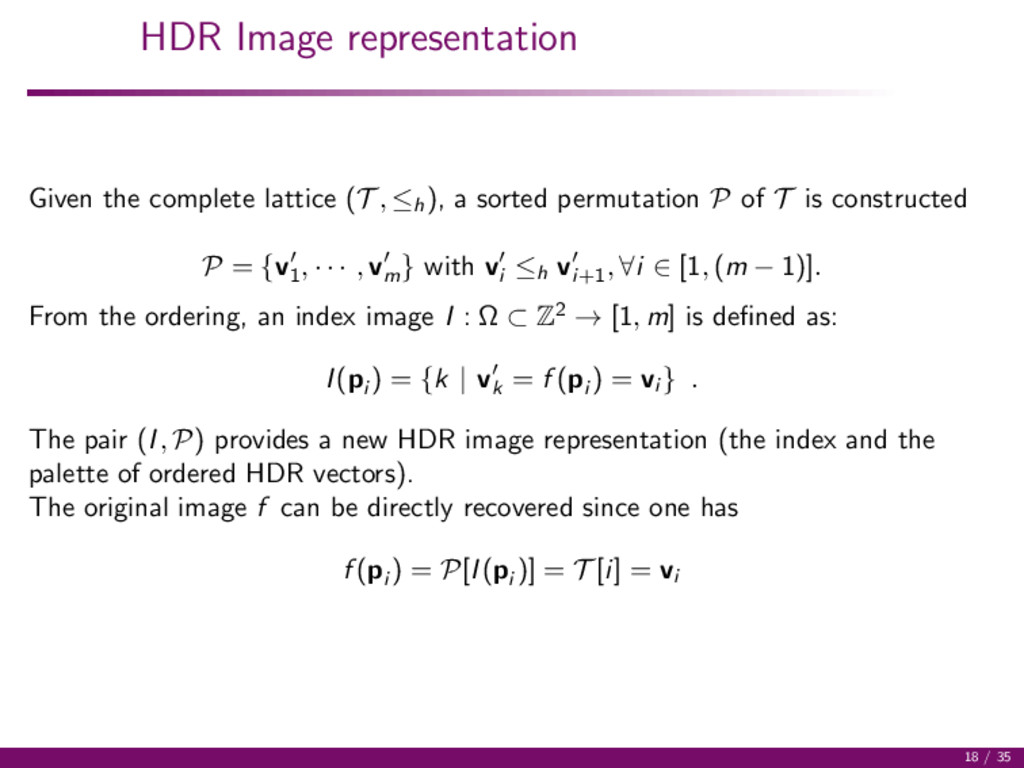
), a sorted permutation P of T is constructed P = {v1 , · · · , vm } with vi ≤h vi+1 , ∀i ∈ [1, (m − 1)]. From the ordering, an index image I : Ω ⊂ Z2 → [1, m] is defined as: I(pi ) = {k | vk = f (pi ) = vi } . The pair (I, P) provides a new HDR image representation (the index and the palette of ordered HDR vectors). The original image f can be directly recovered since one has f (pi ) = P[I(pi )] = T [i] = vi 18 / 35
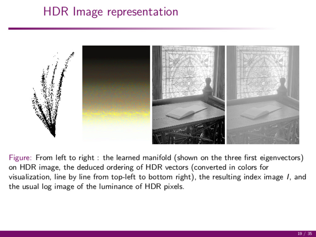
learned manifold (shown on the three first eigenvectors) on HDR image, the deduced ordering of HDR vectors (converted in colors for visualization, line by line from top-left to bottom right), the resulting index image I, and the usual log image of the luminance of HDR pixels. 19 / 35
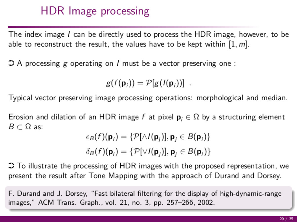
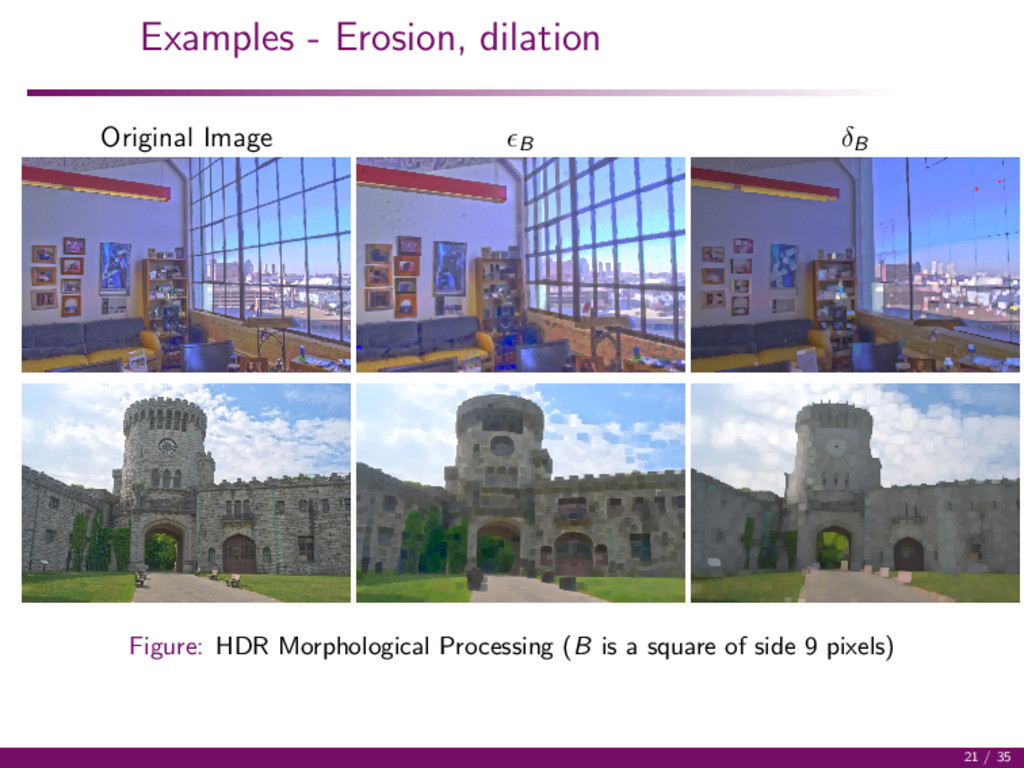
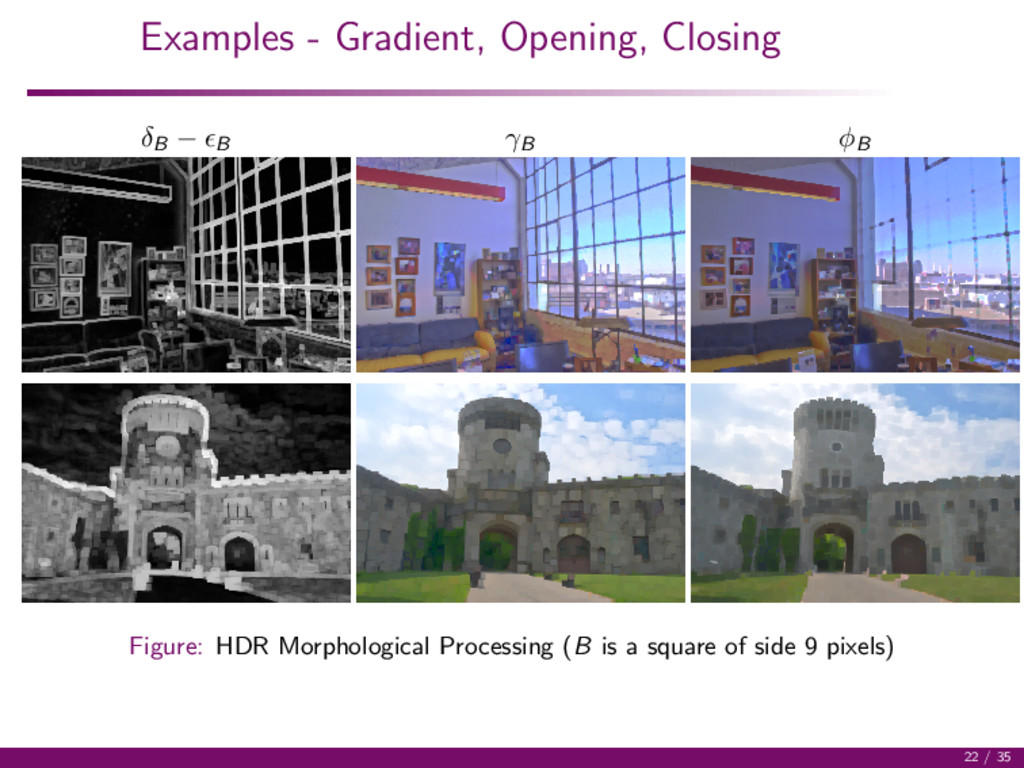
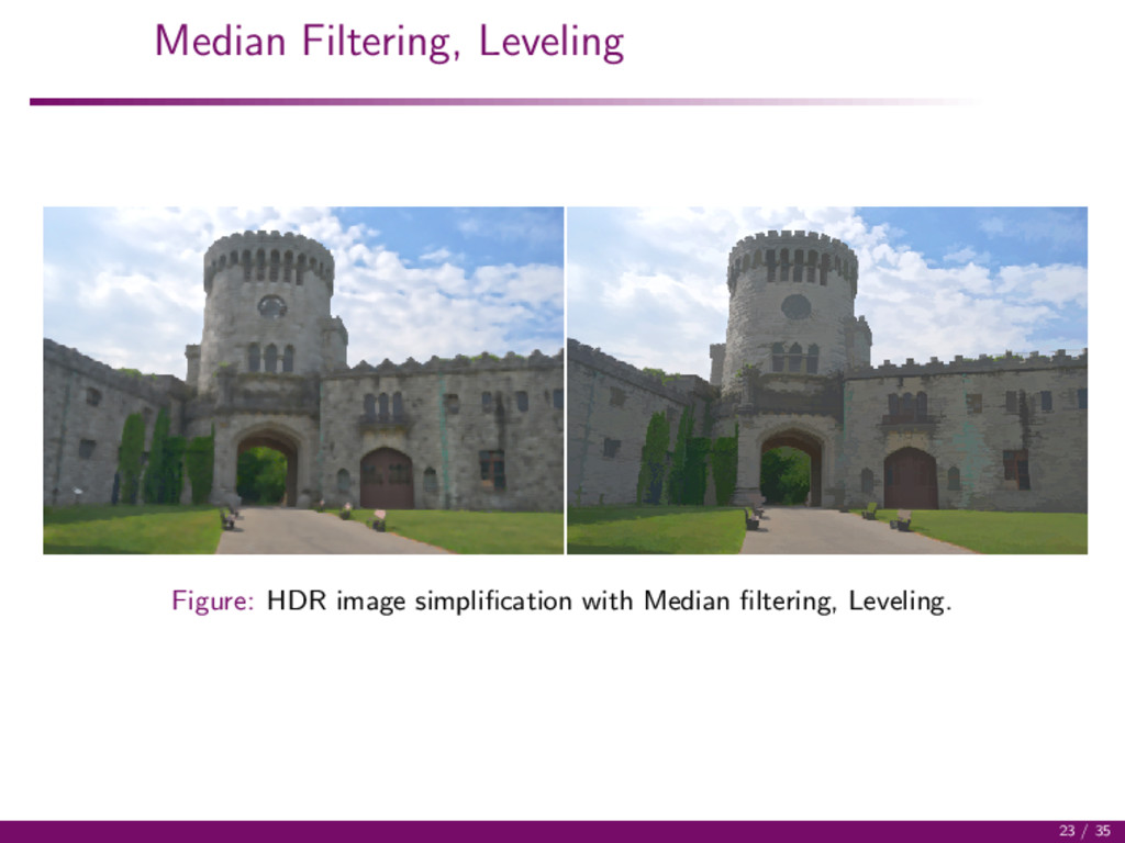
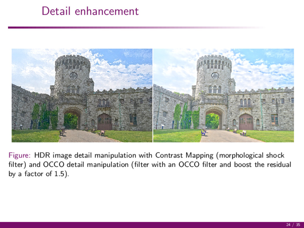
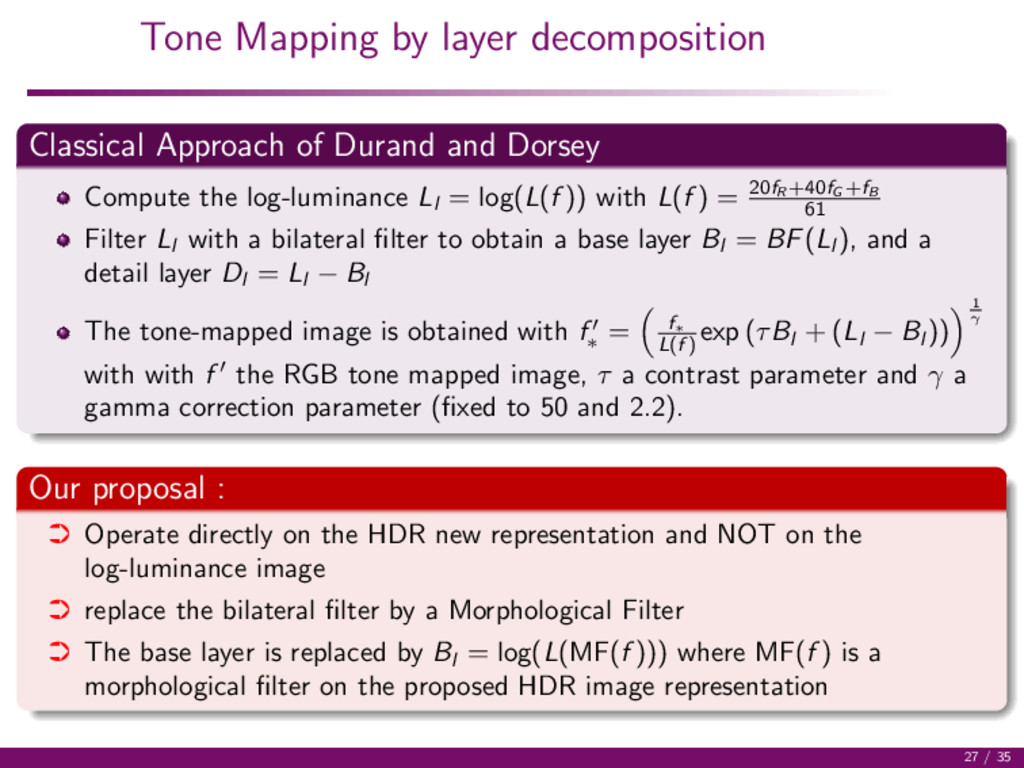
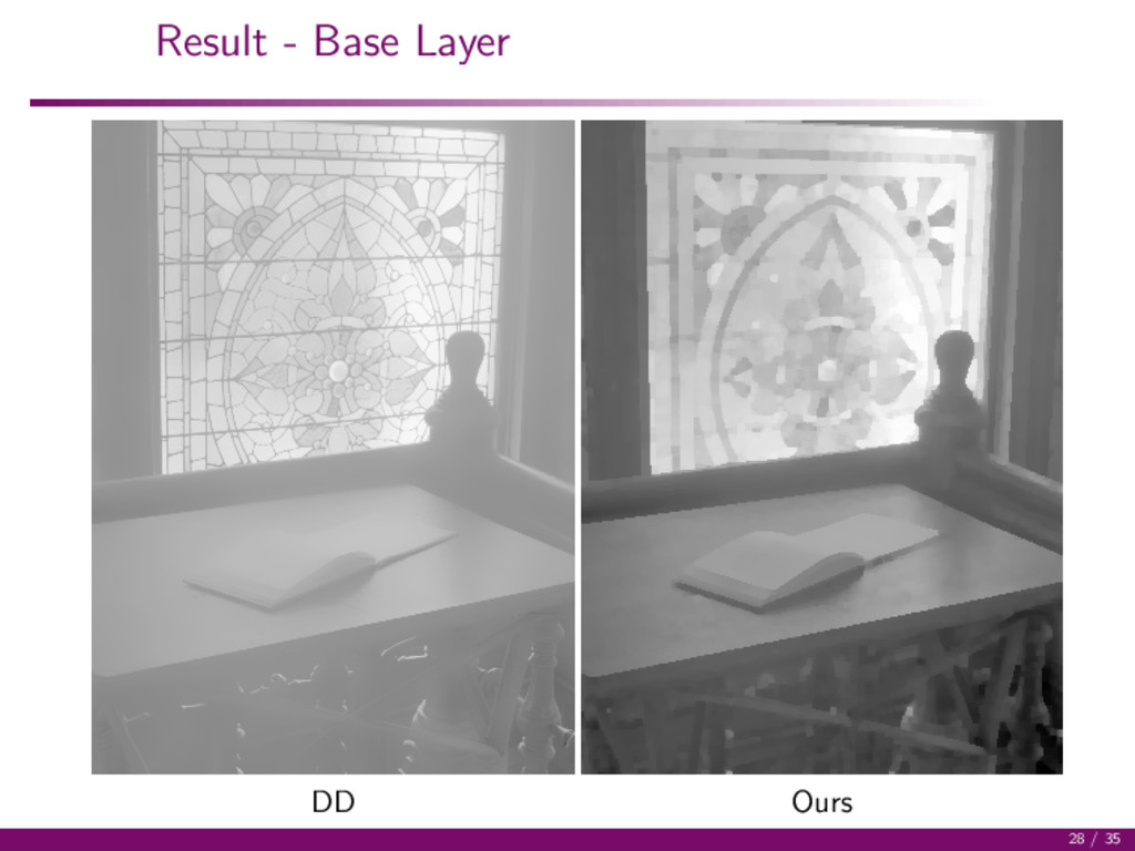
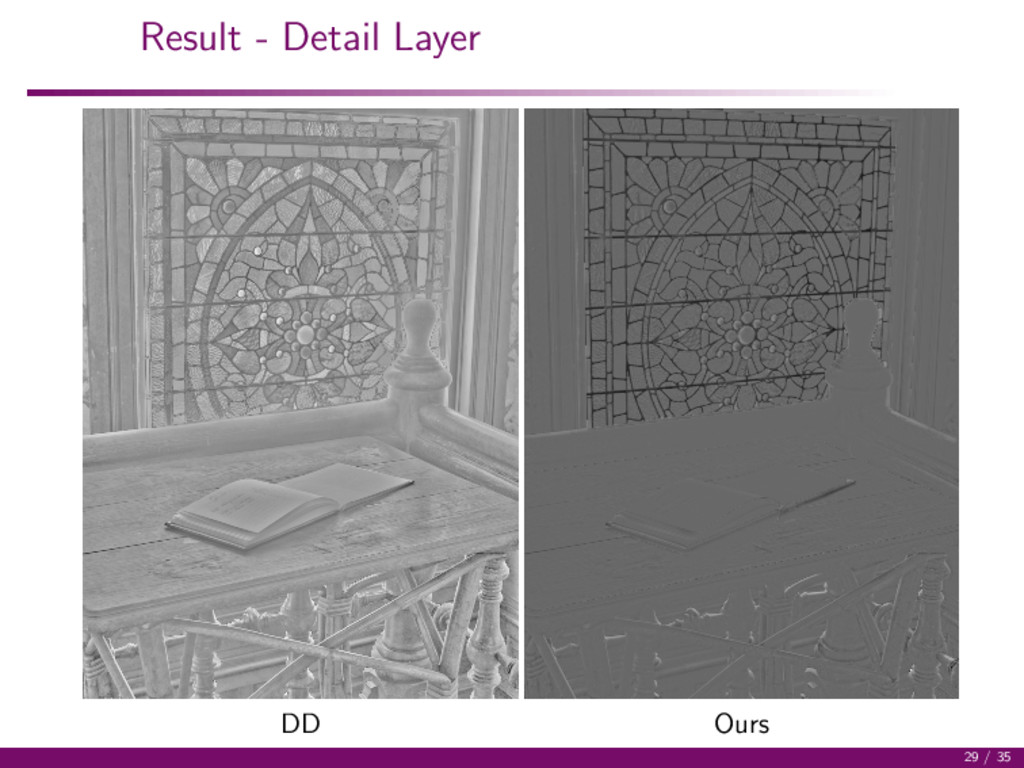
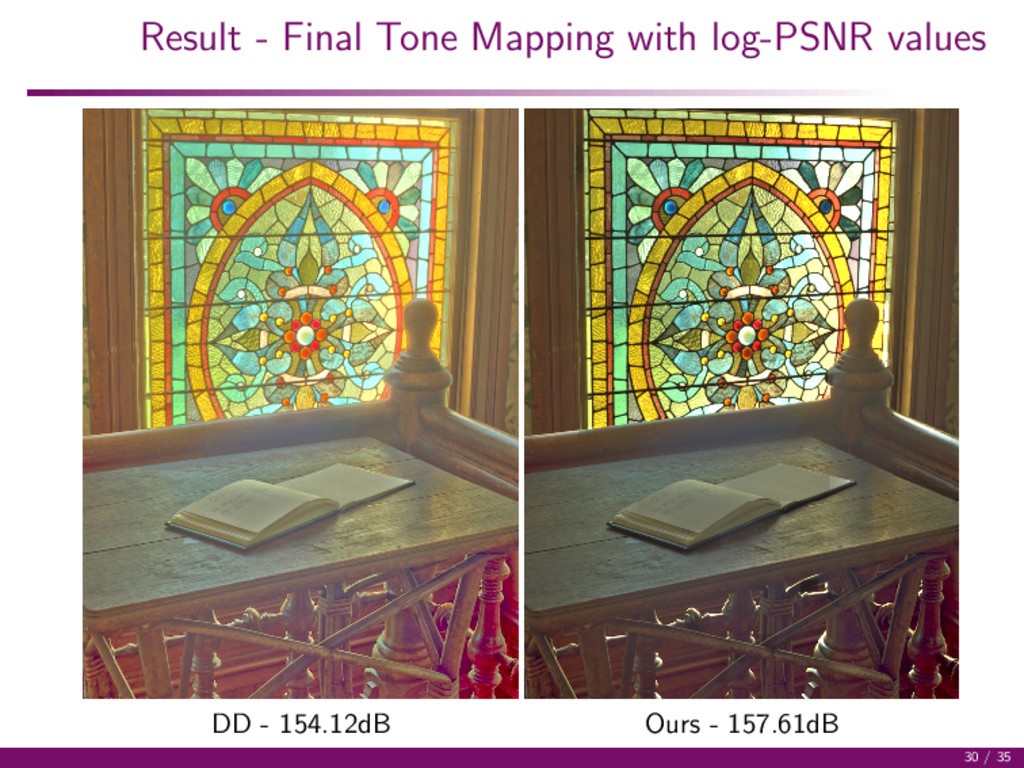
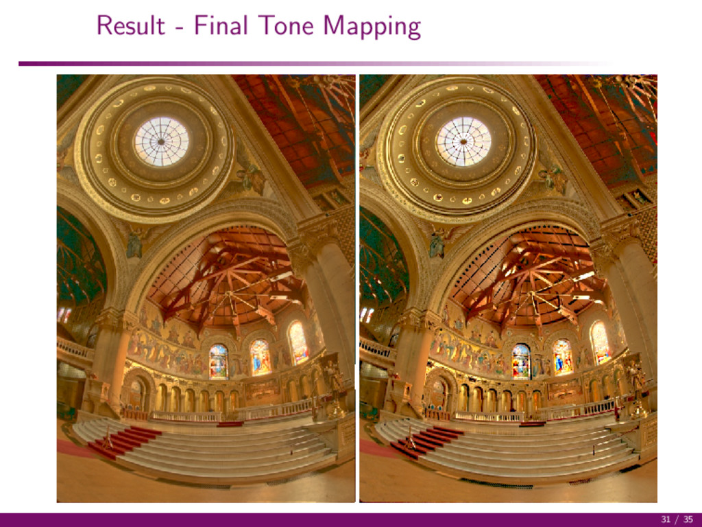
used to process the HDR image, however, to be able to reconstruct the result, the values have to be kept within [1, m]. · A processing g operating on I must be a vector preserving one : g(f (pi )) = P[g(I(pi ))] . Typical vector preserving image processing operations: morphological and median. Erosion and dilation of an HDR image f at pixel pi ∈ Ω by a structuring element B ⊂ Ω as: B (f )(pi ) = {P[∧I(pj )], pj ∈ B(pi )} δB (f )(pi ) = {P[∨I(pj )], pj ∈ B(pi )} · To illustrate the processing of HDR images with the proposed representation, we present the result after Tone Mapping with the approach of Durand and Dorsey. F. Durand and J. Dorsey, “Fast bilateral filtering for the display of high-dynamic-range images,” ACM Trans. Graph., vol. 21, no. 3, pp. 257–266, 2002. 20 / 35
Dorsey Compute the log-luminance Ll = log(L(f )) with L(f ) = 20fR +40fG +fB 61 Filter Ll with a bilateral filter to obtain a base layer Bl = BF(Ll ), and a detail layer Dl = Ll − Bl The tone-mapped image is obtained with f∗ = f∗ L(f ) exp (τBl + (Ll − Bl )) 1 γ with with f the RGB tone mapped image, τ a contrast parameter and γ a gamma correction parameter (fixed to 50 and 2.2). Our proposal : · Operate directly on the HDR new representation and NOT on the log-luminance image · replace the bilateral filter by a Morphological Filter · The base layer is replaced by Bl = log(L(MF(f ))) where MF(f ) is a morphological filter on the proposed HDR image representation 27 / 35
in the form of an index and a palette The palette is obtained by ordering the HDR vectors using a manifold-based ordering, and an index is deduced from it. Vector-preserving operations have been proposed for the processing of raw HDR images. The processing can be used to filter or enhance the images or even for Tone Mapping. · Consider non vector-preserving methods by processing the palette instead of the index image. 34 / 35