My first presentation as a PhD student in which I outline the background to my research project. This presentation was given as part of the University of Southampton Transportation Research Group seminar programme.
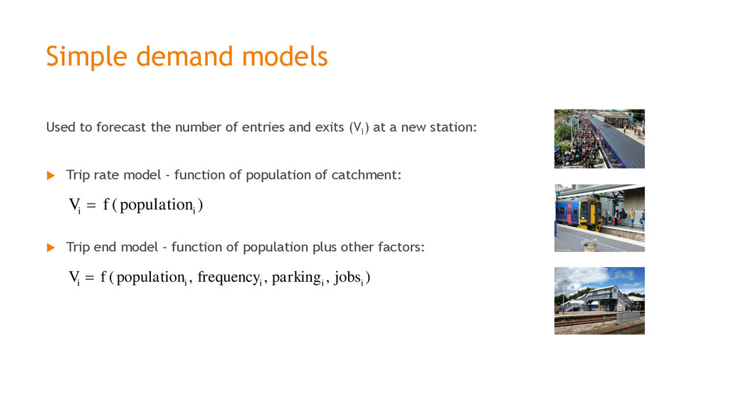
and exits (Vi ) at a new station: Trip rate model - function of population of catchment: Trip end model - function of population plus other factors: ( ) i i V f population ( , , , ) i i i i i V f population frequency parking jobs
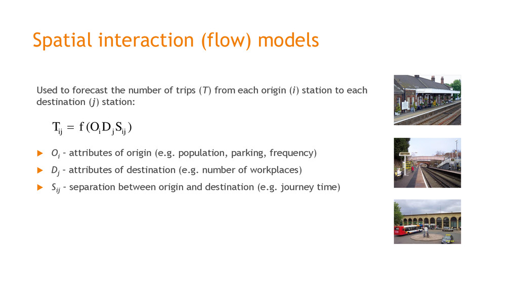
trips (T) from each origin (i) station to each destination (j) station: Oi – attributes of origin (e.g. population, parking, frequency) Dj – attributes of destination (e.g. number of workplaces) Sij – separation between origin and destination (e.g. journey time) ( ) ij i j ij T f O D S
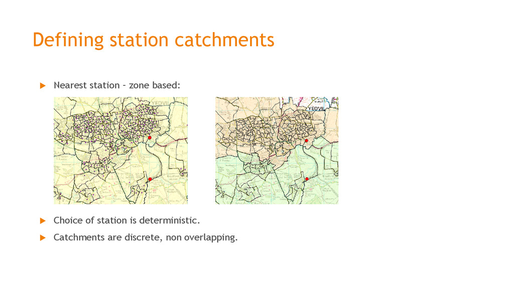
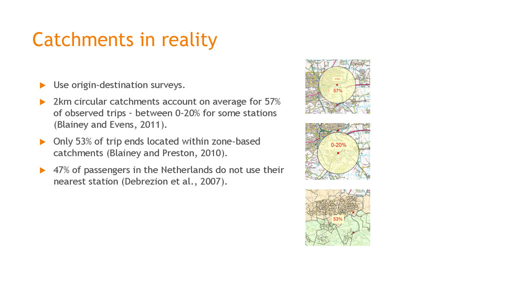
catchments account on average for 57% of observed trips – between 0-20% for some stations (Blainey and Evens, 2011). Only 53% of trip ends located within zone-based catchments (Blainey and Preston, 2010). 47% of passengers in the Netherlands do not use their nearest station (Debrezion et al., 2007).
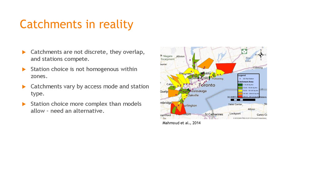
and stations compete. Station choice is not homogenous within zones. Catchments vary by access mode and station type. Station choice more complex than models allow – need an alternative. Mahmoud et al., 2014
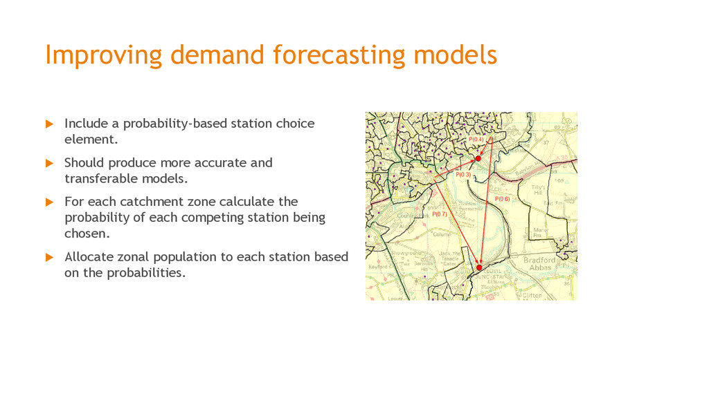
element. Should produce more accurate and transferable models. For each catchment zone calculate the probability of each competing station being chosen. Allocate zonal population to each station based on the probabilities.
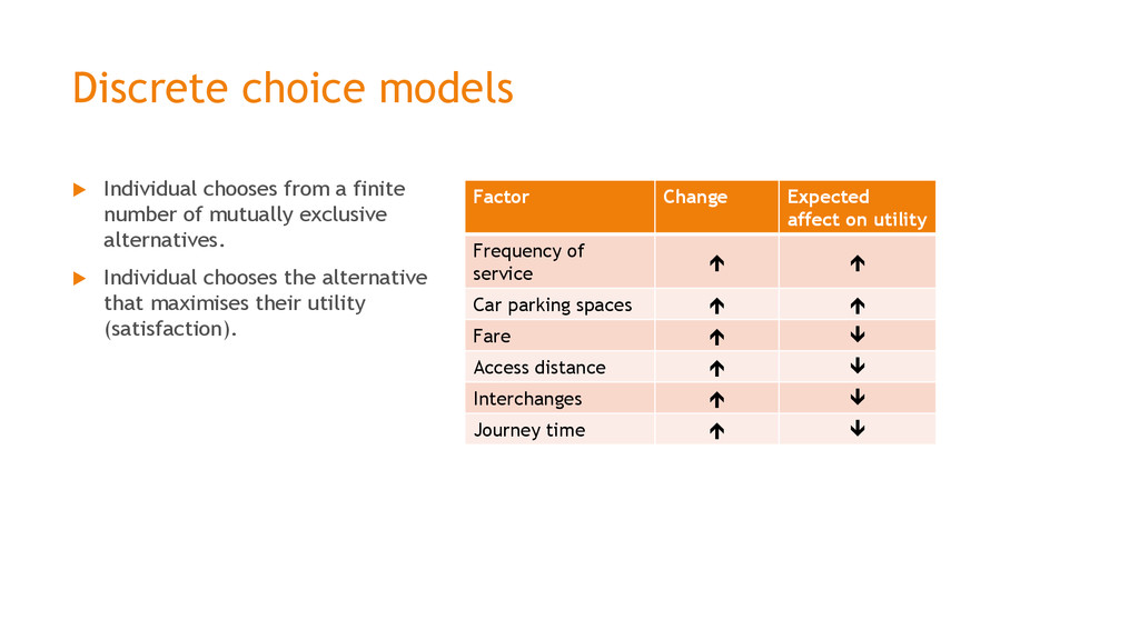
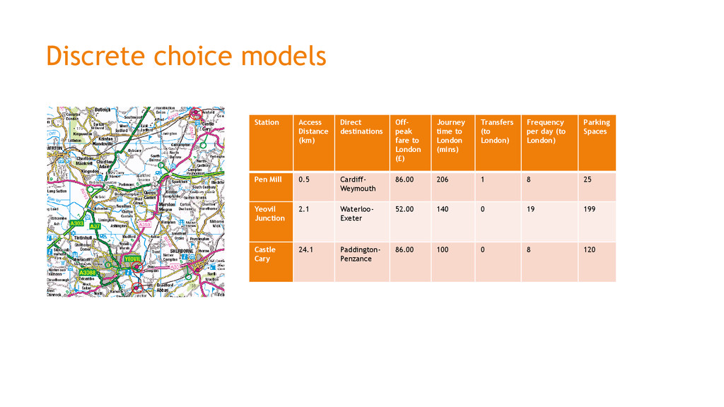
of mutually exclusive alternatives. Individual chooses the alternative that maximises their utility (satisfaction). Factor Change Expected affect on utility Frequency of service Car parking spaces Fare Access distance Interchanges Journey time
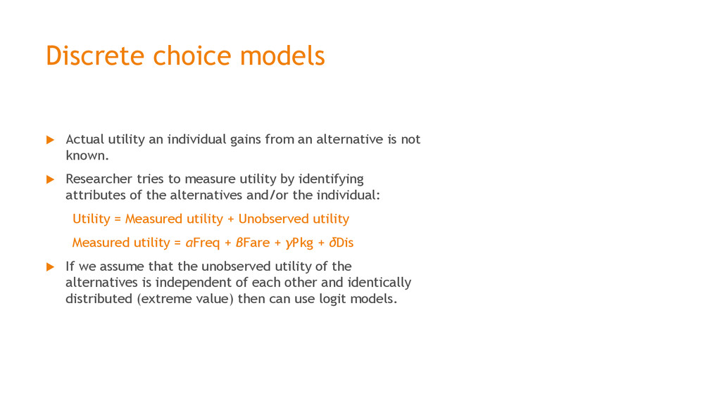
an alternative is not known. Researcher tries to measure utility by identifying attributes of the alternatives and/or the individual: Utility = Measured utility + Unobserved utility Measured utility = αFreq + βFare + γPkg + δDis If we assume that the unobserved utility of the alternatives is independent of each other and identically distributed (extreme value) then can use logit models.
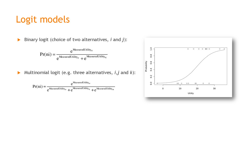
and j): Multinomial logit (e.g. three alternatives, i,j and k): Pr( ) ni nj ni MeasuredUtility MeasuredUtility MeasuredUtility e ni e e Pr( ) ni nj ni nk MeasuredUtility MeasuredUtility MeasuredUtility MeasuredUtility e ni e e e
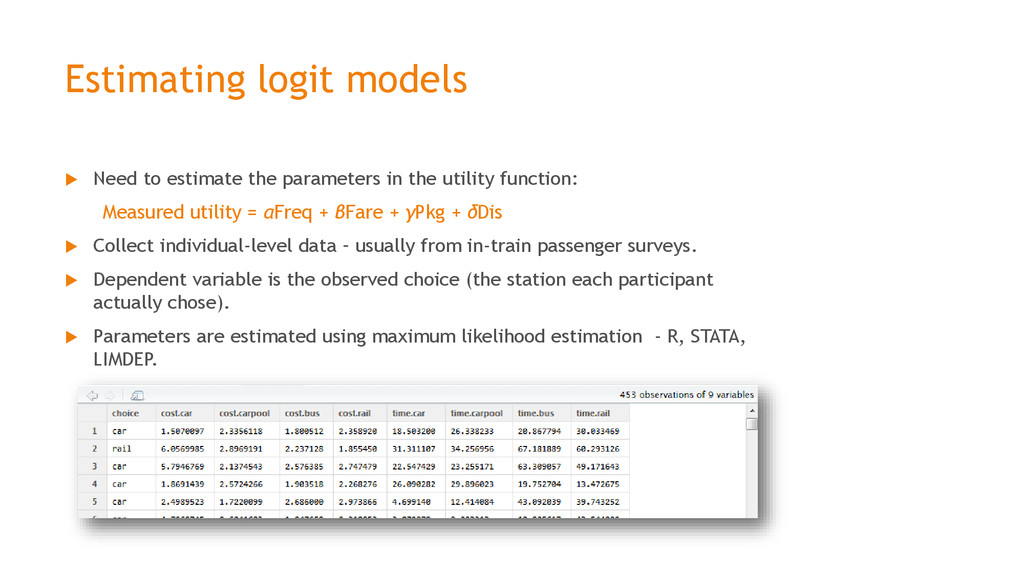
the utility function: Measured utility = αFreq + βFare + γPkg + δDis Collect individual-level data – usually from in-train passenger surveys. Dependent variable is the observed choice (the station each participant actually chose). Parameters are estimated using maximum likelihood estimation - R, STATA, LIMDEP.
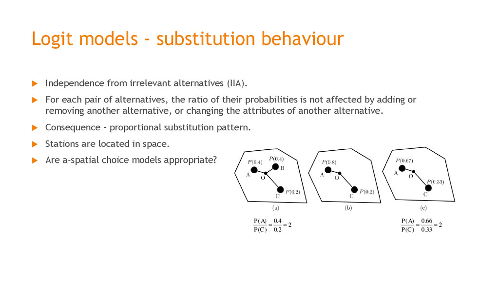
(IIA). For each pair of alternatives, the ratio of their probabilities is not affected by adding or removing another alternative, or changing the attributes of another alternative. Consequence – proportional substitution pattern. Stations are located in space. Are a-spatial choice models appropriate? ( ) 0.4 2 ( ) 0.2 P A P C ( ) 0.66 2 ( ) 0.33 P A P C
of Departure Station by Railway Users,” European Transport, 37, 78–92. Blainey, S. P. and Preston, J. M. (2010) “Modelling Local Rail Demand in South Wales,” Transportation Planning and Technology, 33, 55–73. Blainey, S. and Evens, S. (2011) “Local Station Catchments: Reconciling Theory with Reality.” In European Transport Conference. Mahmoud, M. S., Eng, P. and Shalaby, A. (2014) “Park-and-Ride Access Station Choice Model for Cross-Regional Commuter Trips in the Greater Toronto and Hamilton Area (GTHA).” In Transportation Research Board 93rd Annual Meeting. 50K Raster [TIFF geospatial data], Ordnance Survey (GB), Using: EDINA Digimap Ordnance Survey Service, <http://edina.ac.uk/digimap>, Downloaded: April 2015. 250K Raster [TIFF geospatial data], Ordnance Survey (GB), Using: EDINA Digimap Ordnance Survey Service, <http://edina.ac.uk/digimap>, Downloaded: April 2015.