MLCon 2021

Transcript

1. 17.11.2020 by Łukasz Gebel & Piotr Czajka
2. achine Learning: The Bare Math Behind Libraries 23.06.2021 by Łukasz Gebel & Piotr Czajka
3. Super Heroes & Super Powers
5. Agenda • What is Machine Learning? • Supervised learning • Unsupervised learning • Q&A
6. Machine Learning „Field of study that gives computers the ability to learn without being explicitly programmed.” Arthur Samuel
7. Machine Learning „I consider every method that needs training as intelligent or machine learning method.” Our Lecturer
8. Supervised learning • It is similar to be tought by a teacher.
9. Supervised learning • Build your model that performs particular task: – Prepare data set consisting of examples & expected outputs
10. Supervised learning • Build your model that performs particular task: – Prepare data set consisting of examples & expected outputs – Present examples to your model
11. Supervised learning • Build your model that performs particular task: – Prepare data set consisting of examples & expected outputs – Present examples to your model – Check how it responds (model’s output values)
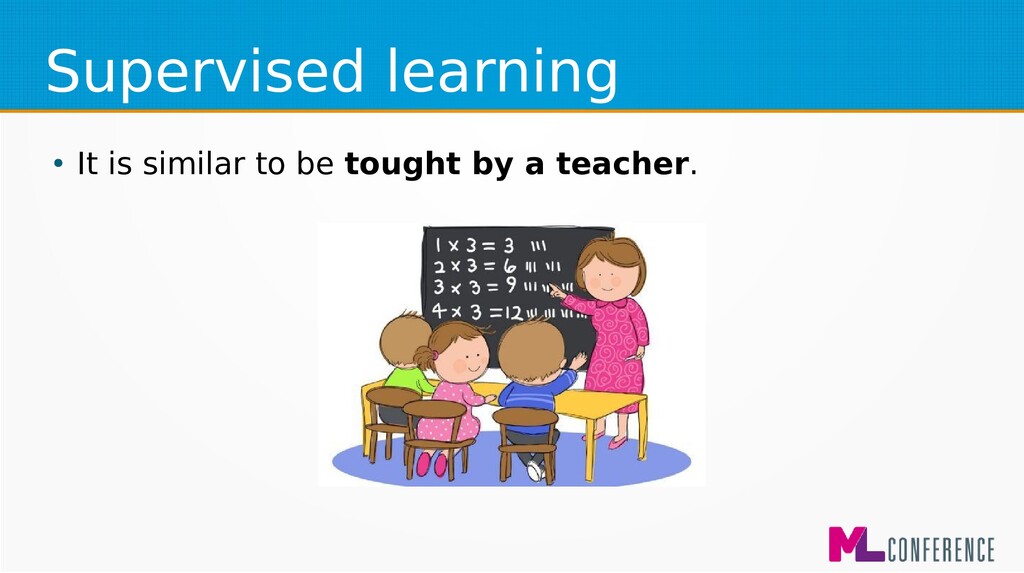
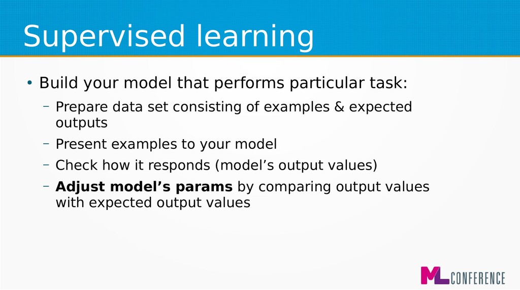
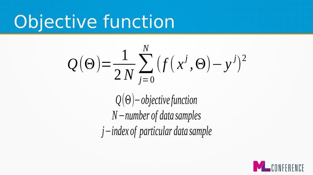
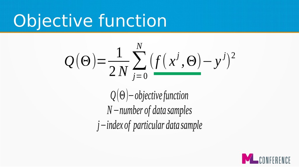
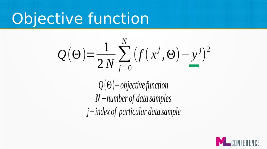
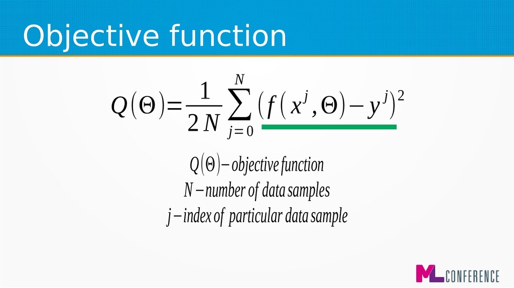
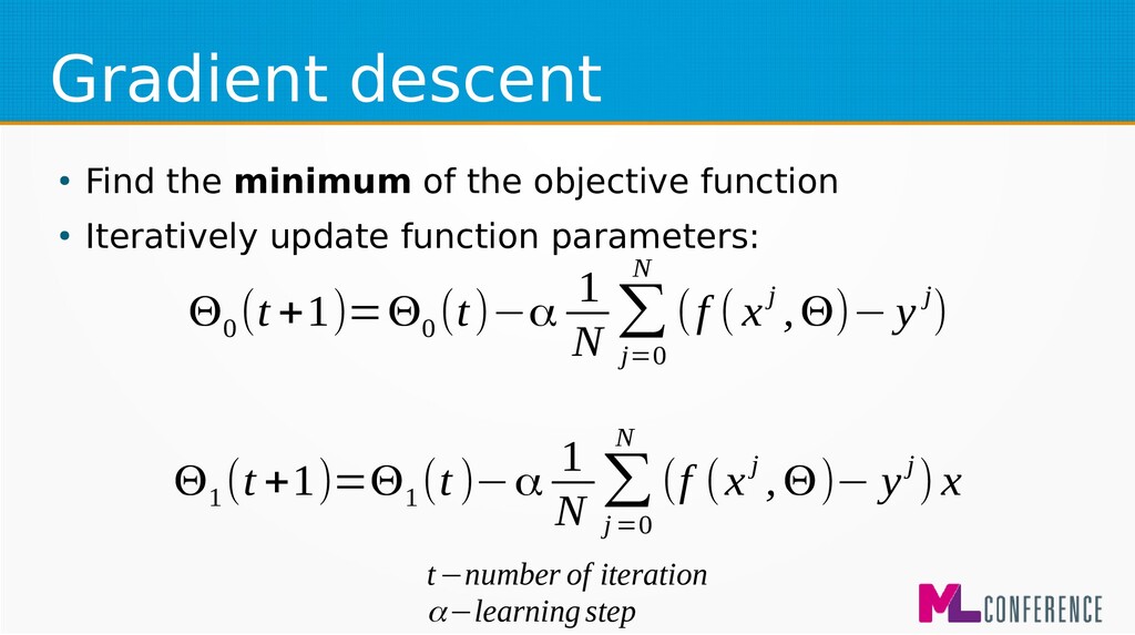
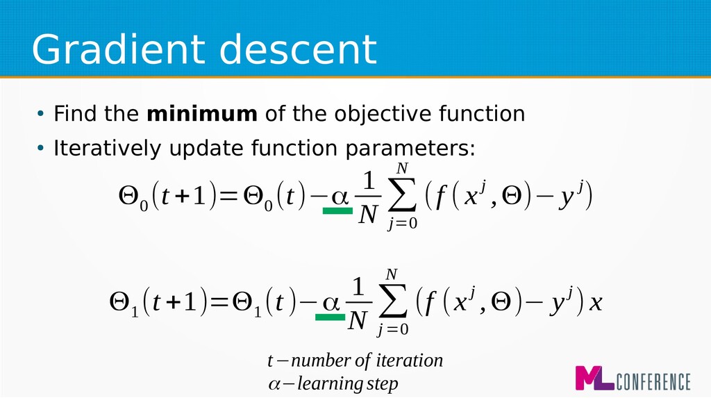
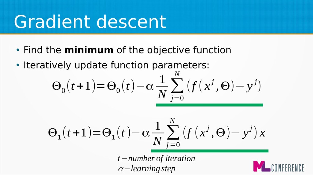
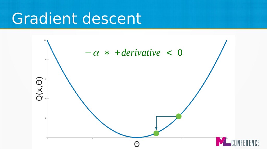
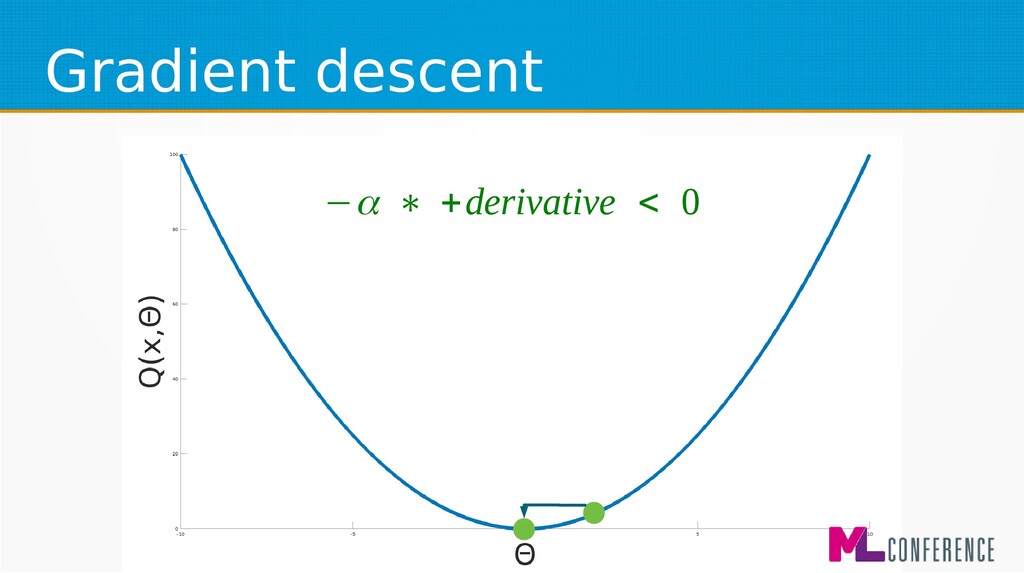
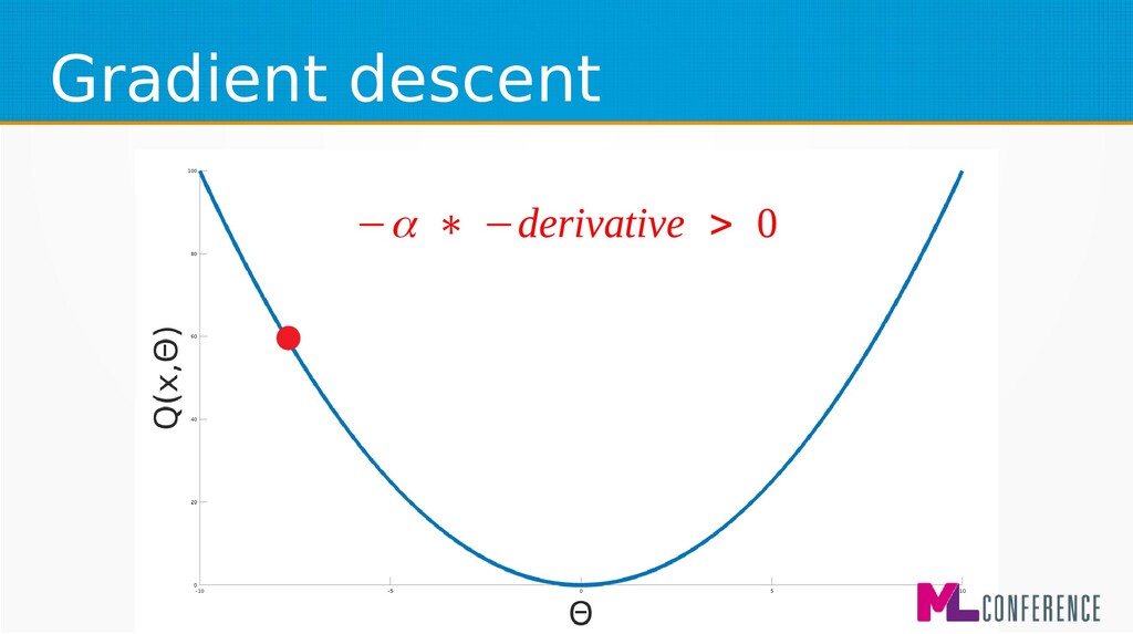
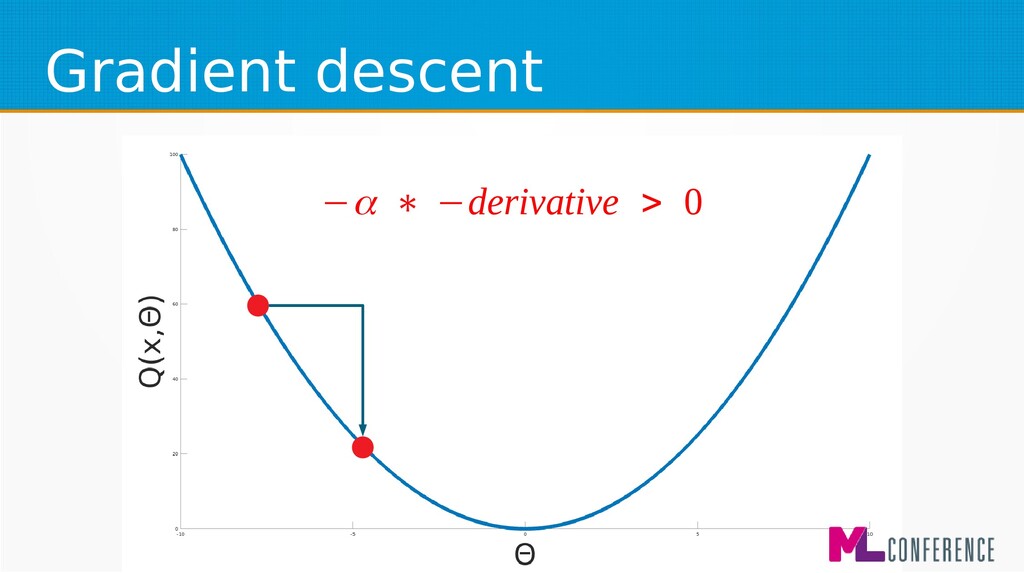
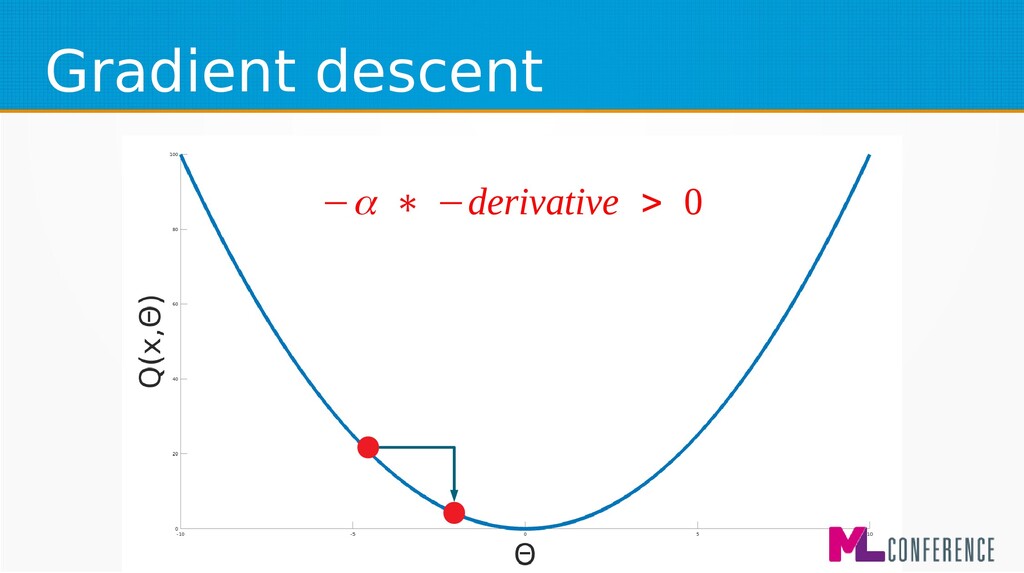
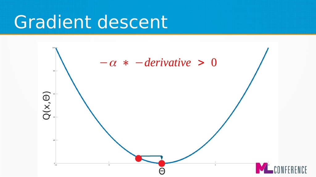
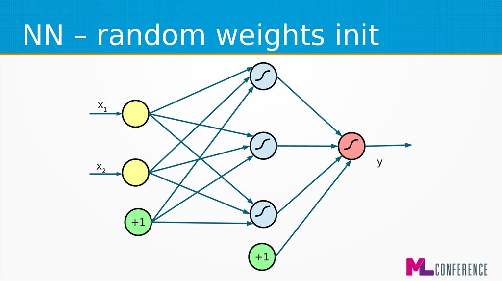
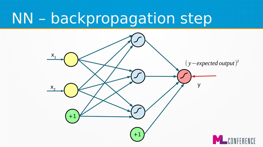
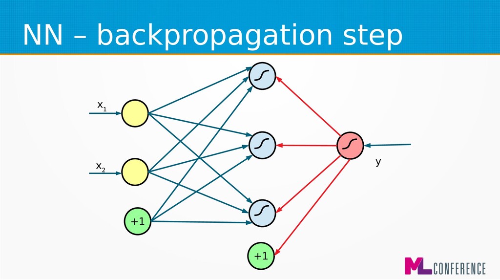
12. Supervised learning • Build your model that performs particular task: – Prepare data set consisting of examples & expected outputs – Present examples to your model – Check how it responds (model’s output values) – Adjust model’s params by comparing output values with expected output values
13. Neural Networks • Inspired by biological brain mechanisms • Many applications: – Computer vision – Speech recognition – Compression
14. Biological Neuron http://www.marekrei.com/blog/wp-content/uploads/2014/01/neuron.png
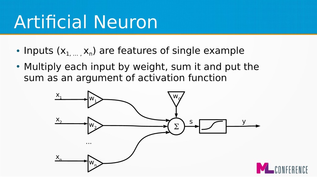
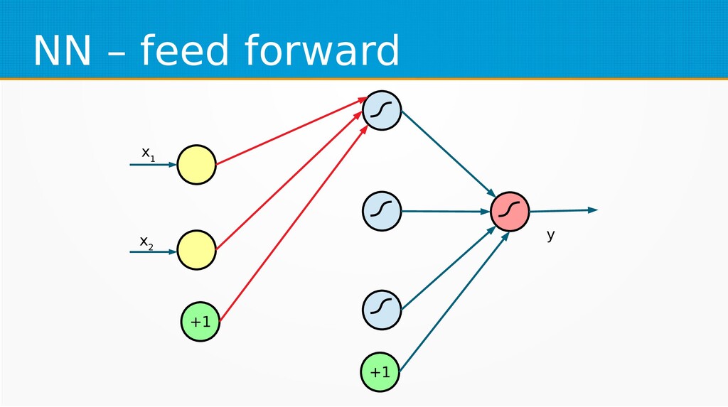
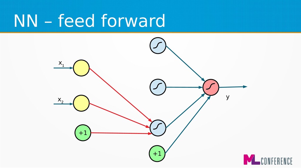
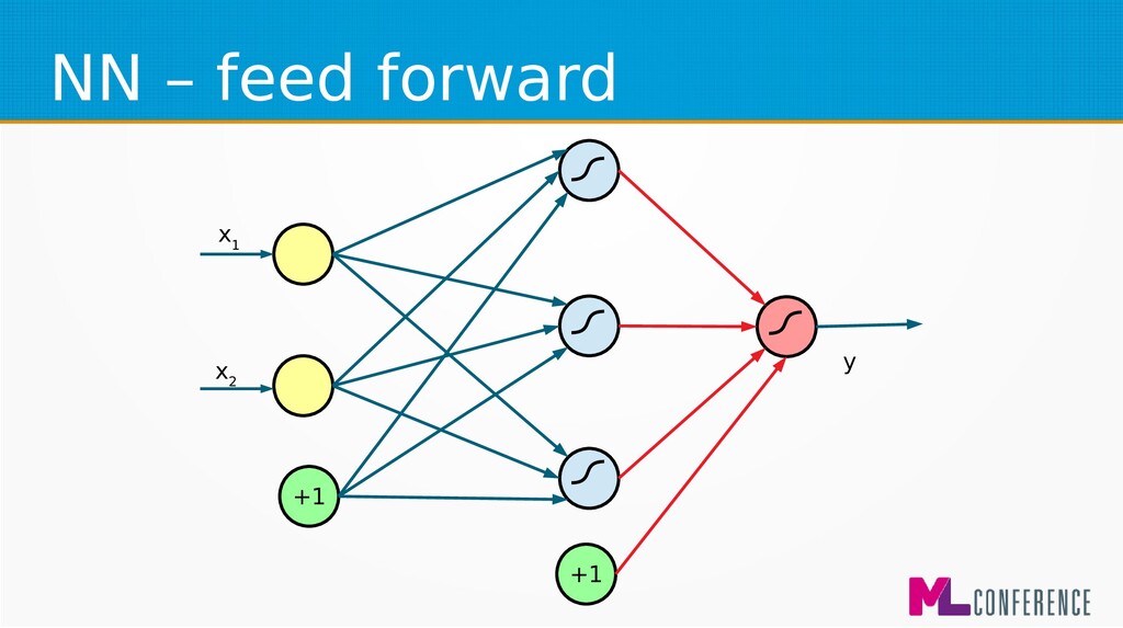
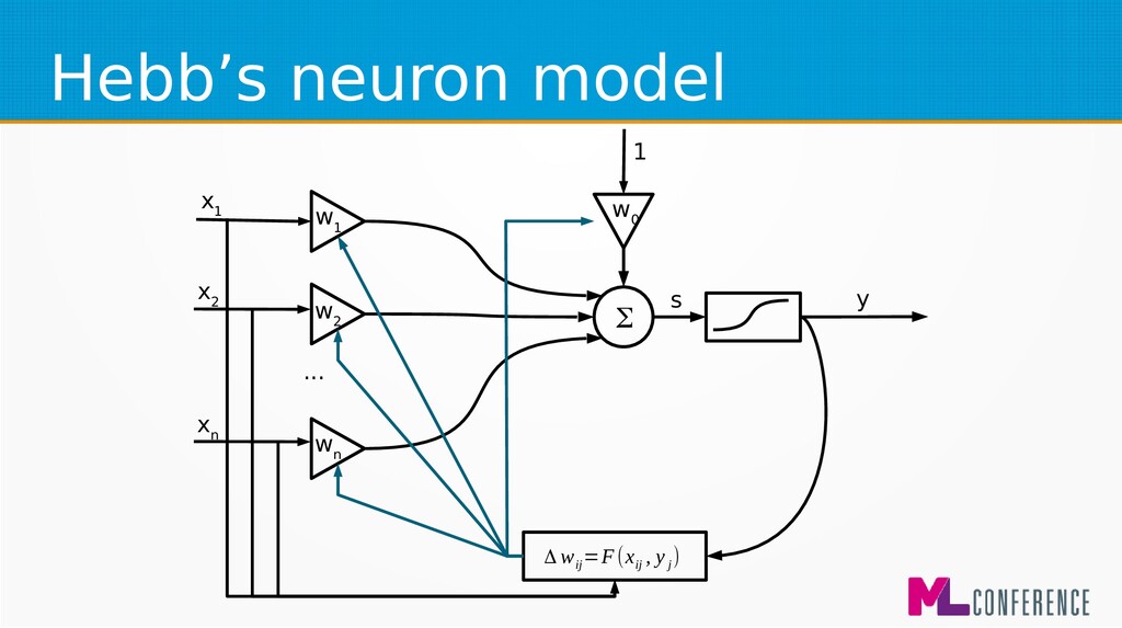
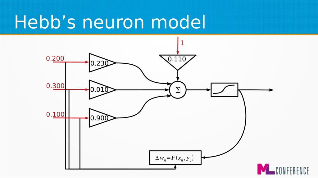
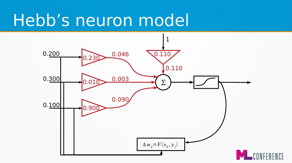
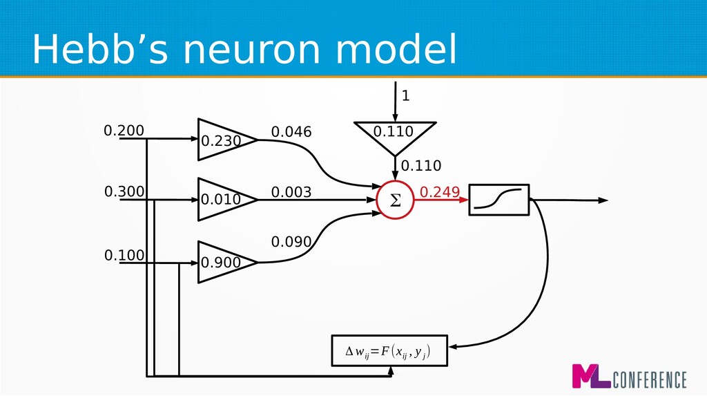
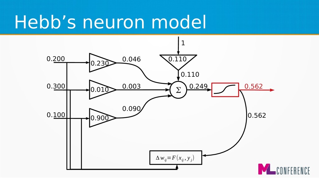
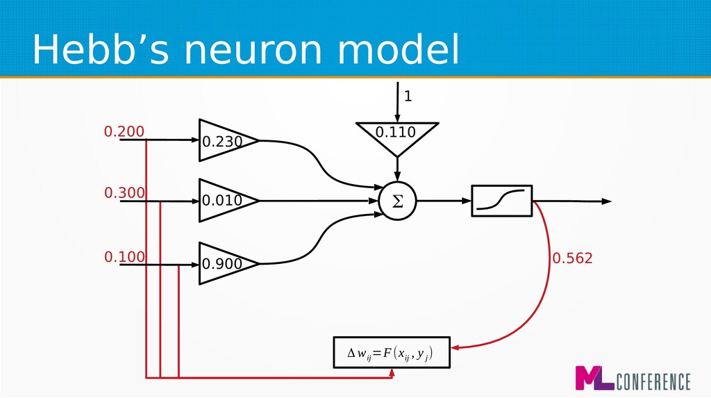
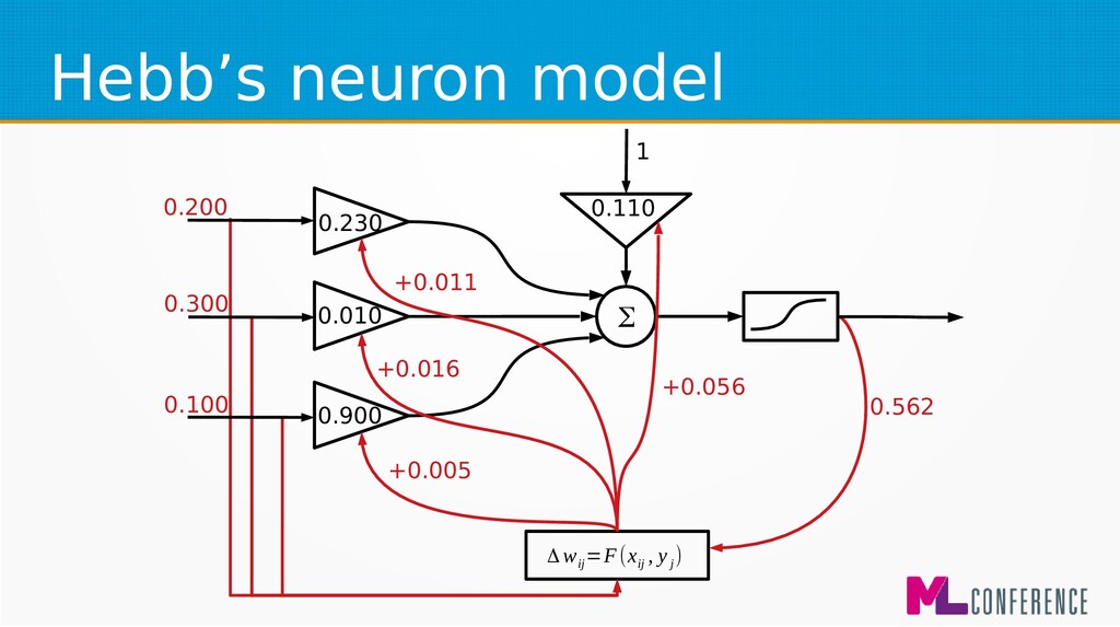
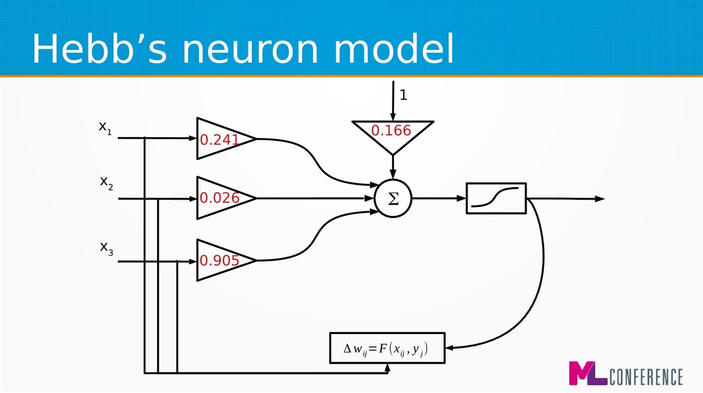
15. Artificial Neuron • Inputs (x 1, … , x n ) are features of single example • Multiply each input by weight, sum it and put the sum as an argument of activation function w 1 w 2 w n w 0 Σ x 1 x 2 x n ... s y
16. Activation function • Sigmoid – Maps sum of neurons signals to value from 0 to 1 – Continous, nonlinear – If input is positive it gives values > 0.5 f (x)= 1 1+e(−βx)
17. Linear Regression • Method for modelling relationship between variables • Simplest form: how x relates to y • Examples: – House size vs house price – Voltage vs electric current
18. Real life problem
19. What defines a superhero?
20. Costume
21. Costume
22. Costume price vs number of issues • For given amount of money predict in how many comic book issues you’ll appear. Costume price(x) Number of issues (y) 240 6370 480 8697 ... ... 26 2200
23. Interesting fact • Invisible woman costume costs $120 Invisible woman
24. Linear regression • Let's have a function: f (x ,Θ)=Θ1 x+Θ0 f (x,Θ)−number of comicbookissues x−costume price Θ−parameters
25. Let's plot
26. Let's plot
27. Let's plot
28. Warning!
29. Objective function Q(Θ)= 1 2 N ∑ j=0 N (f ( xj ,Θ)−y j )2 Q(Θ)−objectivefunction N−numberof datasamples j−indexof particulardatasample
30. Objective function Q(Θ)= 1 2 N ∑ j=0 N (f ( xj ,Θ)−y j )2 Q(Θ)−objectivefunction N−numberof datasamples j−indexof particulardatasample
31. Objective function Q(Θ)= 1 2 N ∑ j=0 N (f ( xj ,Θ)−y j )2 Q(Θ)−objectivefunction N−numberof datasamples j−indexof particulardatasample
32. Objective function Q(Θ)= 1 2 N ∑ j=0 N (f ( xj ,Θ)−y j )2 Q(Θ)−objectivefunction N−numberof datasamples j−indexof particulardatasample
33. Objective function - intuition f (xj ,Θ)=4 y=2 (4−2)2 =22 =4 sum+=4
34. Objective function - intuition f (xj ,Θ)=1 y=1 (1−1)2 =02 =0 sum+=0
35. Gradient descent • Find the minimum of the objective function • Iteratively update function parameters: Θ0 (t +1)=Θ0 (t)−α 1 N ∑ j=0 N (f ( xj ,Θ)− y j ) Θ1 (t +1)=Θ1 (t )−α 1 N ∑ j=0 N (f (xj ,Θ)− yj ) x t−number of iteration α−learning step
36. Gradient descent • Find the minimum of the objective function • Iteratively update function parameters: Θ0 (t +1)=Θ0 (t)−α 1 N ∑ j=0 N (f ( xj ,Θ)− y j ) Θ1 (t +1)=Θ1 (t )−α 1 N ∑ j=0 N (f (xj ,Θ)− yj ) x t−number of iteration α−learning step
37. Gradient descent • Find the minimum of the objective function • Iteratively update function parameters: Θ0 (t +1)=Θ0 (t)−α 1 N ∑ j=0 N (f ( xj ,Θ)− y j ) Θ1 (t +1)=Θ1 (t )−α 1 N ∑ j=0 N (f (xj ,Θ)− yj ) x t−number of iteration α−learning step
38. Gradient descent
39. Gradient descent −α ∗ +derivative < 0
40. Gradient descent −α ∗ +derivative < 0
41. Gradient descent −α ∗ +derivative < 0
42. Gradient descent −α ∗ +derivative < 0
43. Gradient descent −α ∗ −derivative > 0
44. Gradient descent −α ∗ −derivative > 0
45. Gradient descent −α ∗ −derivative > 0
46. Gradient descent −α ∗ −derivative > 0
47. Demo
48. Linearly separable problem
49. Not linearly separable problem
50. NN – random weights init +1 +1 x 1 x 2 y
51. NN – feed forward +1 +1 x 1 x 2 y
52. NN – feed forward +1 +1 x 1 x 2 y
53. NN – feed forward +1 +1 x 1 x 2 y
54. NN – feed forward +1 +1 x 1 x 2 y
55. NN – compute error +1 +1 x 1 x 2 y ( y−expected output)2
56. NN – backpropagation step • Use gradient descent and computed error • Update every weight of every neuron from hidden and output layer
57. NN – backpropagation step +1 +1 x 1 x 2 y ( y−expected output)2
58. NN – backpropagation step +1 +1 x 1 x 2 y
59. Neural Network „Neural networks are nothing more than randomized optimization.” Another Lecturer
60. Real life problem • You said it can solve non linear problems, let's generate superhero logo using it.
61. Unsupervised learning
62. What? They can learn by themselves?
63. What? They can learn by themselves?
64. Why would we let them? • Less complex mathematical apparatus than in supervised learning. • It is similar to discovering world on your own.
65. Why would we let them? Used mostly for sorting and grouping when: • Sorting key can’t be easily figured out. • Data is very complex and finding the key is not trivial.
66. Idea behind – groups
67. Idea behind – groups
68. Idea behind – groups
69. Hebbian learning
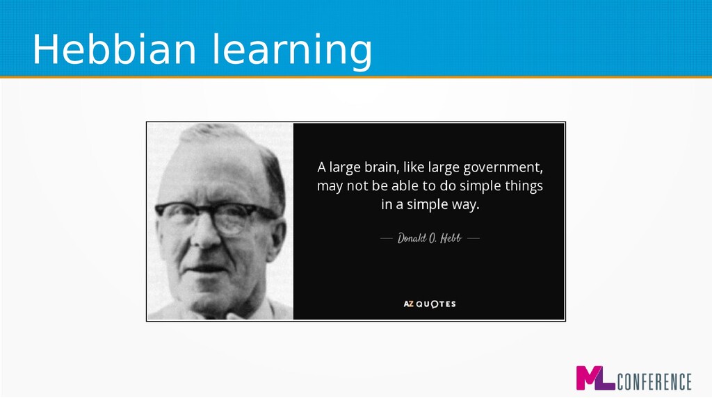
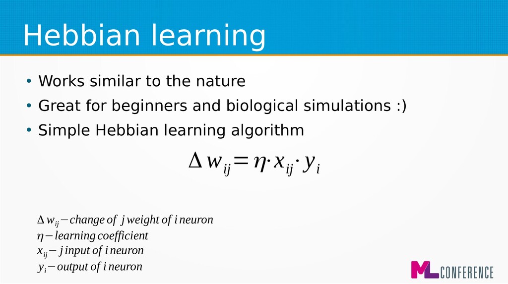
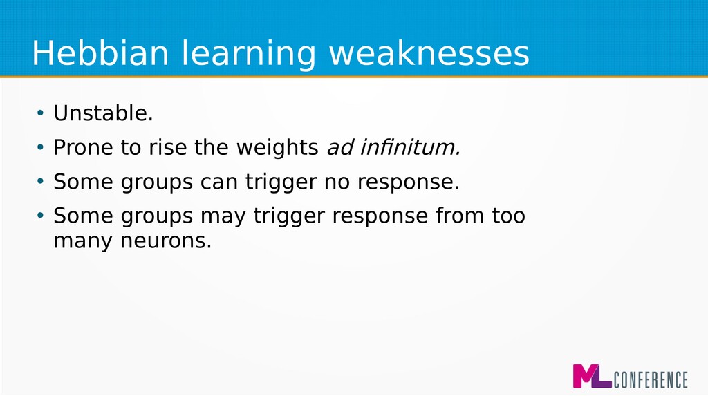
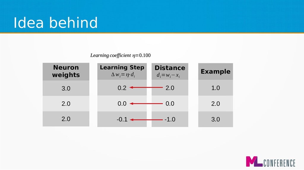
70. Hebbian learning • Works similar to the nature • Great for beginners and biological simulations :) • Simple Hebbian learning algorithm Δ w ij =η⋅x ij ⋅y i Δ w ij −change of j weight of ineuron η−learningcoefficient x ij − jinput of ineuron y i −output of i neuron
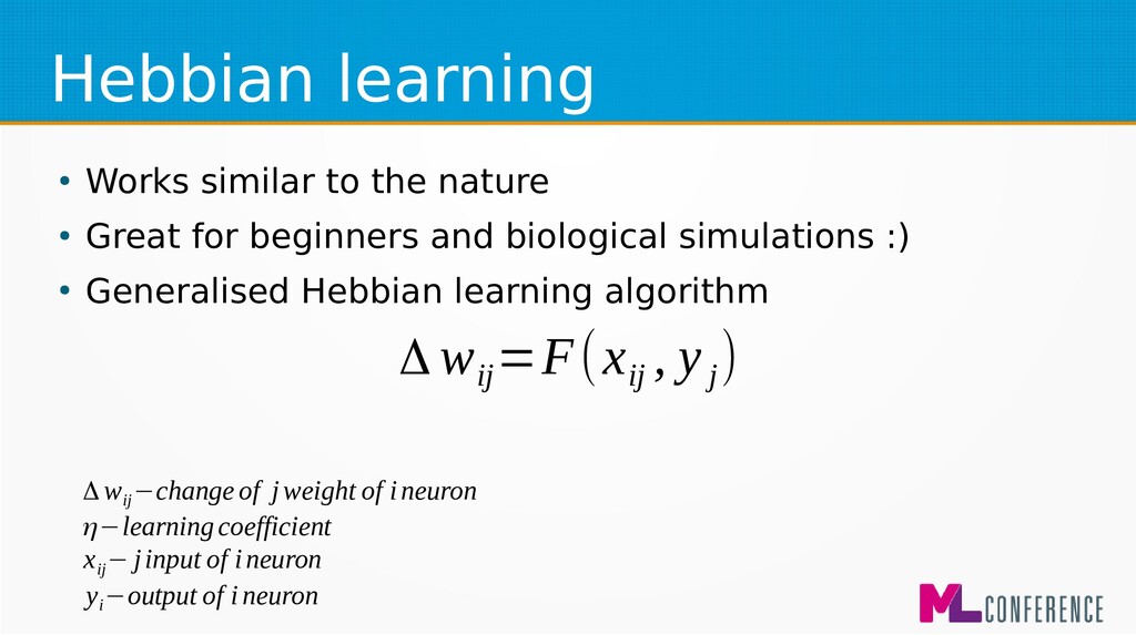
71. Hebbian learning • Works similar to the nature • Great for beginners and biological simulations :) • Generalised Hebbian learning algorithm Δ w ij =F(x ij , y j ) Δ w ij −change of j weight of ineuron η−learningcoefficient x ij − jinput of ineuron y i −output of i neuron
72. Hebb’s neuron model w 1 w 2 w n w 0 Δ w ij =F(x ij , y j ) Σ x 1 x 2 x n ... 1 s y
73. Hebb’s neuron model 0.230 0.010 0.900 0.110 Δ w ij =F(x ij , y j ) Σ 0.200 0.300 0.100 1
74. Hebb’s neuron model 0.230 0.010 0.900 0.110 Δ w ij =F(x ij , y j ) Σ 1 0.046 0.003 0.090 0.110 0.200 0.300 0.100
75. Hebb’s neuron model 0.230 0.010 0.900 0.110 Δ w ij =F(x ij , y j ) Σ 1 0.046 0.003 0.090 0.110 0.249 0.200 0.300 0.100
76. Hebb’s neuron model 0.230 0.010 0.900 0.110 Δ w ij =F(x ij , y j ) Σ 1 0.046 0.003 0.090 0.110 0.249 0.562 0.562 0.200 0.300 0.100
77. Hebb’s neuron model 0.230 0.010 0.900 0.110 Δ w ij =F(x ij , y j ) Σ 1 0.562 0.200 0.300 0.100
78. Hebb’s neuron model 0.230 0.010 0.900 0.110 Δ w ij =F(x ij , y j ) Σ 1 0.562 +0.011 +0.016 +0.005 +0.056 0.300 0.100 0.200
79. Hebb’s neuron model 0.241 0.026 0.905 0.166 Δ w ij =F(x ij , y j ) Σ x 1 x 2 x 3 1
80. Demo
81. Imagine superhero teams
82. Marvel database to the rescue Intelligence Strength Speed Durability Energy projection Fighting skills Iron Man 6 6 5 6 6 4 Spiderman 4 4 3 3 1 4 Black Panter 5 3 2 3 3 5 Wolverine 2 4 2 4 1 7 Thor 2 7 7 6 6 4 Dr Strange 4 2 7 2 6 6 Hulk 2 7 3 7 5 4 Cpt. America 3 3 2 3 1 6 Mr Fantastic 6 2 2 5 1 3 Human Torch 2 2 5 2 5 3 Invisible Woman 3 2 3 6 5 3 The Thing 3 6 2 6 1 5 Luke Cage 3 4 2 5 1 4 She Hulk 3 7 3 6 1 4 Ms Marvel 2 6 2 6 1 4 Daredevil 3 3 2 2 4 5
83. Hebbian learning weaknesses • Unstable. • Prone to rise the weights ad infinitum. • Some groups can trigger no response. • Some groups may trigger response from too many neurons.
84. And now – self organising networks
85. Self organising?
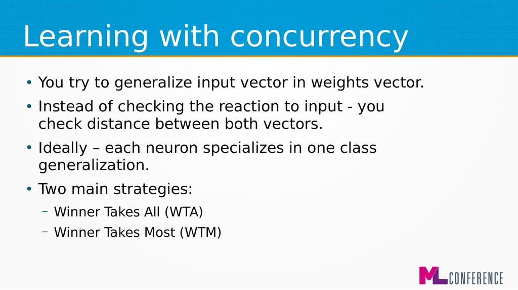
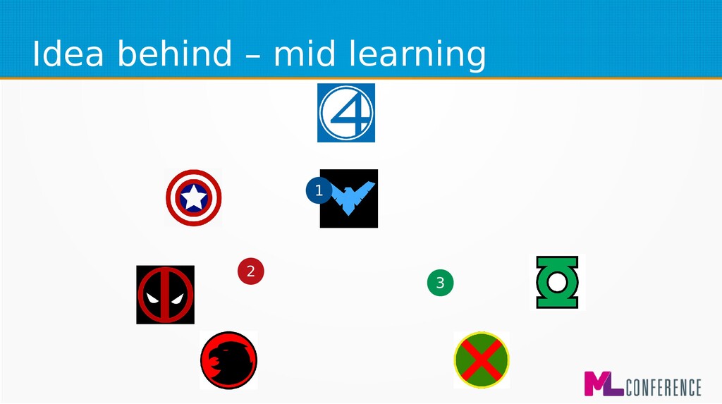
86. Learning with concurrency • You try to generalize input vector in weights vector. • Instead of checking the reaction to input - you check distance between both vectors. • Ideally – each neuron specializes in one class generalization. • Two main strategies: – Winner Takes All (WTA) – Winner Takes Most (WTM)
87. Idea behind Neuron weights 3.0 2.0 2.0 Example 1.0 2.0 3.0
88. Example 1.0 2.0 3.0 Idea behind Distance 2.0 0.0 -1.0 Neuron weights 3.0 2.0 2.0 d i =w i −x i Euclidiandistance √∑ i=1 n d i 2 =√5
89. Distance 2.0 0.0 -1.0 Idea behind Neuron weights 3.0 2.0 2.0 Learning coefficient η=0.100 Learning Step 0.2 0.0 -0.1 Δ w i =η⋅d i Example 1.0 2.0 3.0 d i =w i −x i Learning coefficient η=0.100
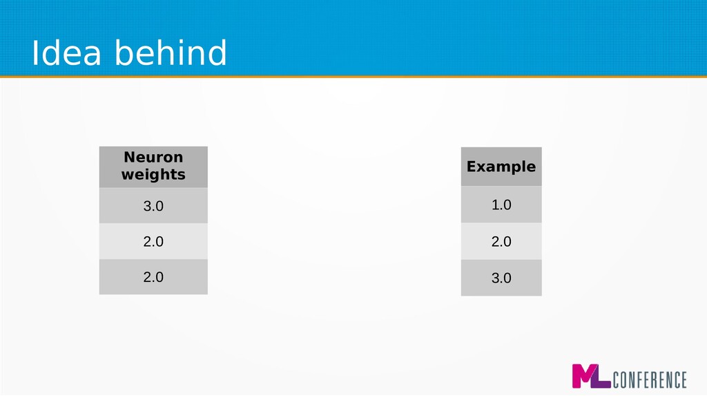
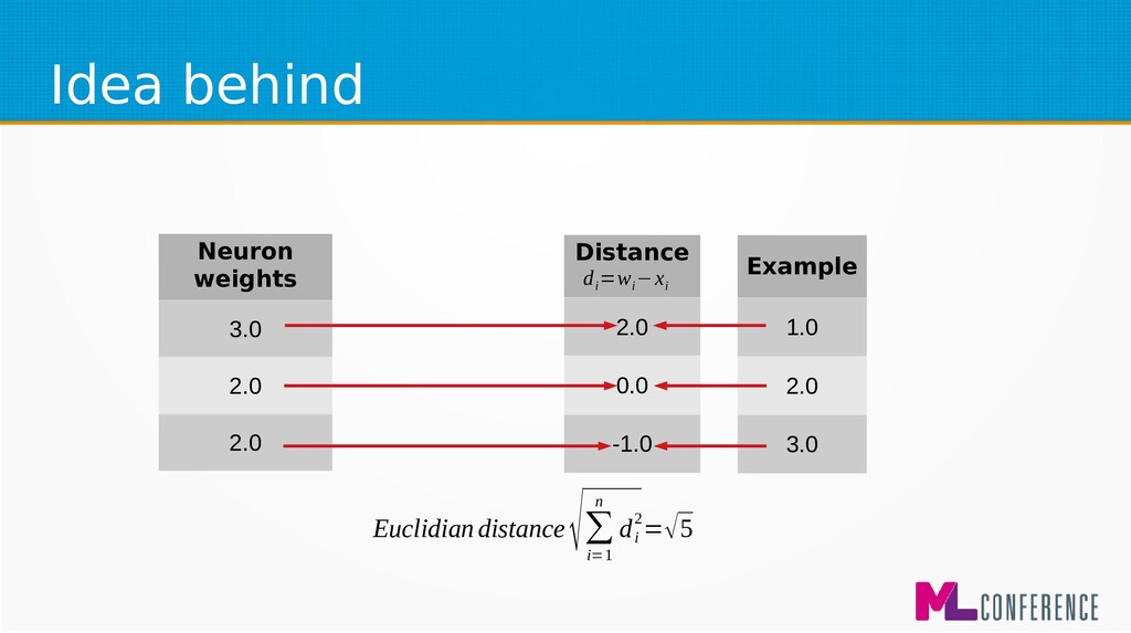
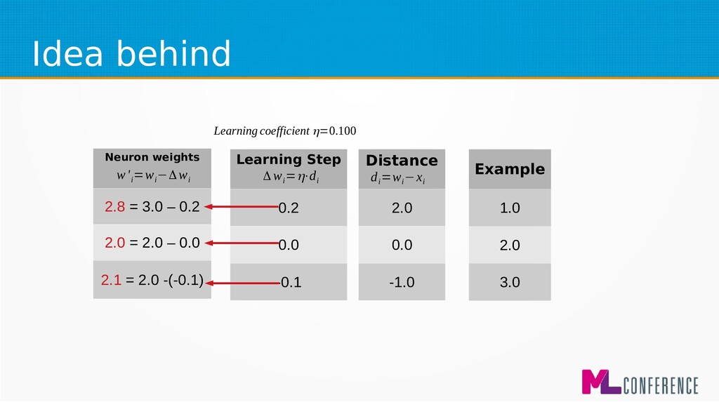
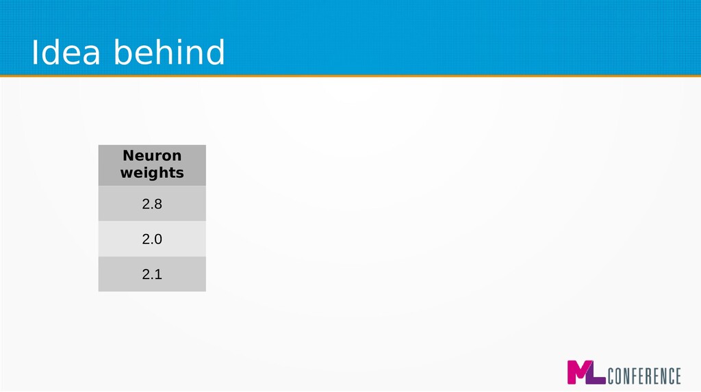
90. Idea behind Distan ce 2.0 0.0 -1.0 Neuron weights 2.8 = 3.0 – 0.2 2.0 = 2.0 – 0.0 2.1 = 2.0 -(-0.1) Exam ple 1.0 2.0 3.0 d i =w i −x i Learning coefficient η=0.100 Learning Step 0.2 0.0 -0.1 w' i =w i −Δw i Δ w i =η⋅d i Example 1.0 2.0 3.0 Learning Step 0.2 0.0 -0.1 Δ w i =η⋅d i Distance 2.0 0.0 -1.0 d i =w i −x i
91. Idea behind Neuron weights 2.8 2.0 2.1
92. Idea behind – initial setup 1 2 3
93. Idea behind – mid learning 1 2 3
94. Idea behind – homeostasis 1 2 3
95. Demo time
96. Learning with concurrency • Gives more diverse groups. • Less prone to clustering (than Hebb’s). • Searches wider spectrum of answers. • First step to more complex networks.
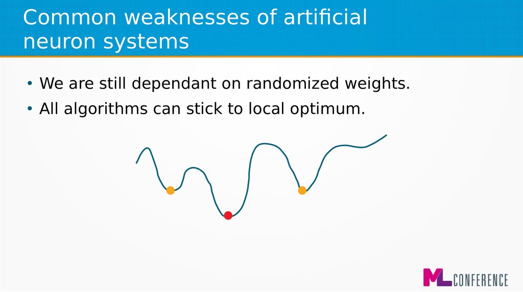
97. Learning with concurency - weaknesses • WTA – works best if teaching examples are evenly distributed in solution space. • WTM – works best if weights’ vectors are evenly distributed in solution space. • Still can stick to local optimum.
98. Teuvo Kohonen’s SOM Created by this nice guy here
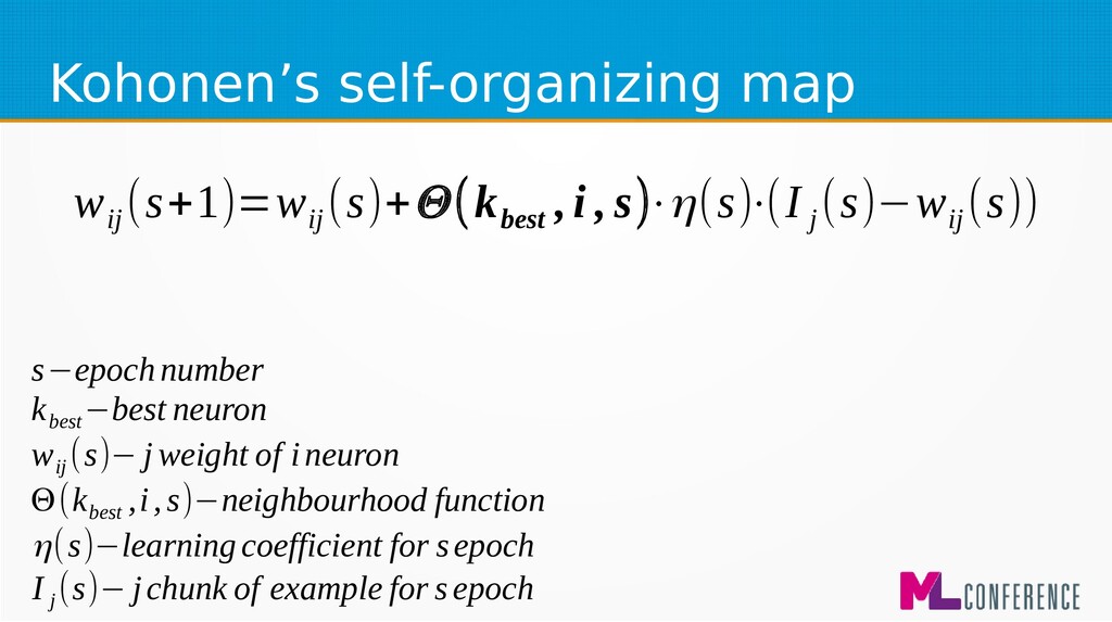
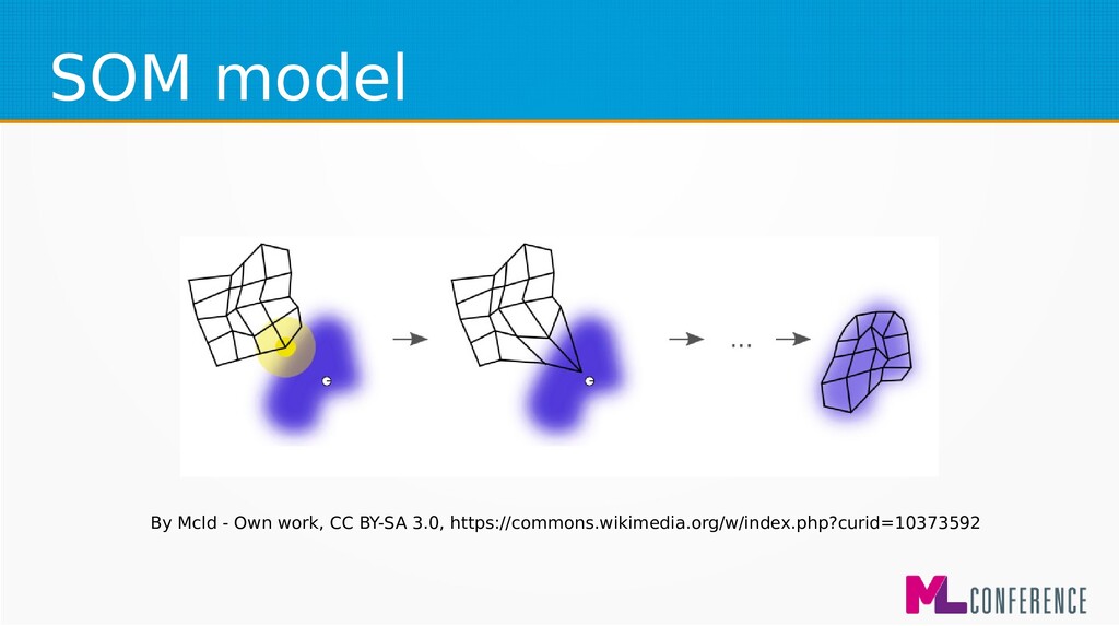
99. Kohonen’s self-organizing map • The most popular self-organizing network with concurrency algorithm. • It teaches groups of neurons with WTM alghoritm • Special features: – Neurons are organised in a grid – Nevertheless – they are treated as a single layer
100. Kohonen’s self-organizing map w ij (s+1)=w ij (s)+Θ(k best ,i , s)⋅η(s)⋅(I j (s)−w ij (s)) s−epochnumber k best −best neuron w ij (s)− j weight of ineuron Θ(k best ,i,s)−neighbourhood function η(s)−learning coefficient for sepoch I j (s)− jchunk of example for s epoch
101. SOM model By Mcld - Own work, CC BY-SA 3.0, https://commons.wikimedia.org/w/index.php?curid=10373592
102. Common weaknesses of artificial neuron systems • We are still dependant on randomized weights. • All algorithms can stick to local optimum.
103. Bibliography • Presentation + code: https://bitbucket.org/medwith/public/downloads/mluvr-MLCon.zip • https://www.coursera.org/learn/machine-learning • https://www.coursera.org/specializations/deep-learning • Math for Machine Learning - Amazon Training and Certification • Linear and Logistic Regression - Amazon Training and Certification • Grus J., Data Science from Scratch: First Principles with Python • Patterson J., Gibson A., Deep Learning: A Practitioner's Approach • Trask A., Grokking Deep Learning • Stroud K. A., Booth D. J, Engineering Mathematics • https://github.com/massie/octave-nn- neural network Octave implementation • https://www.desmos.com/calculator/dnzfajfpym - Nanananana … Batman equation ;) • https://xkcd.com/605/ - extrapolating ;) • http://dilbert.com/strip/2013-02-02 - Dilbert & Machine Learning
104. Thank you