Week, In-Person • New York, San Francisco, Chicago, Seattle • Corporate Training • Python for Data Science • Machine Learning • Natural Language Processing • Spark • Evening Professional Development Courses • Explore Data Science Online Training thisismetis.com
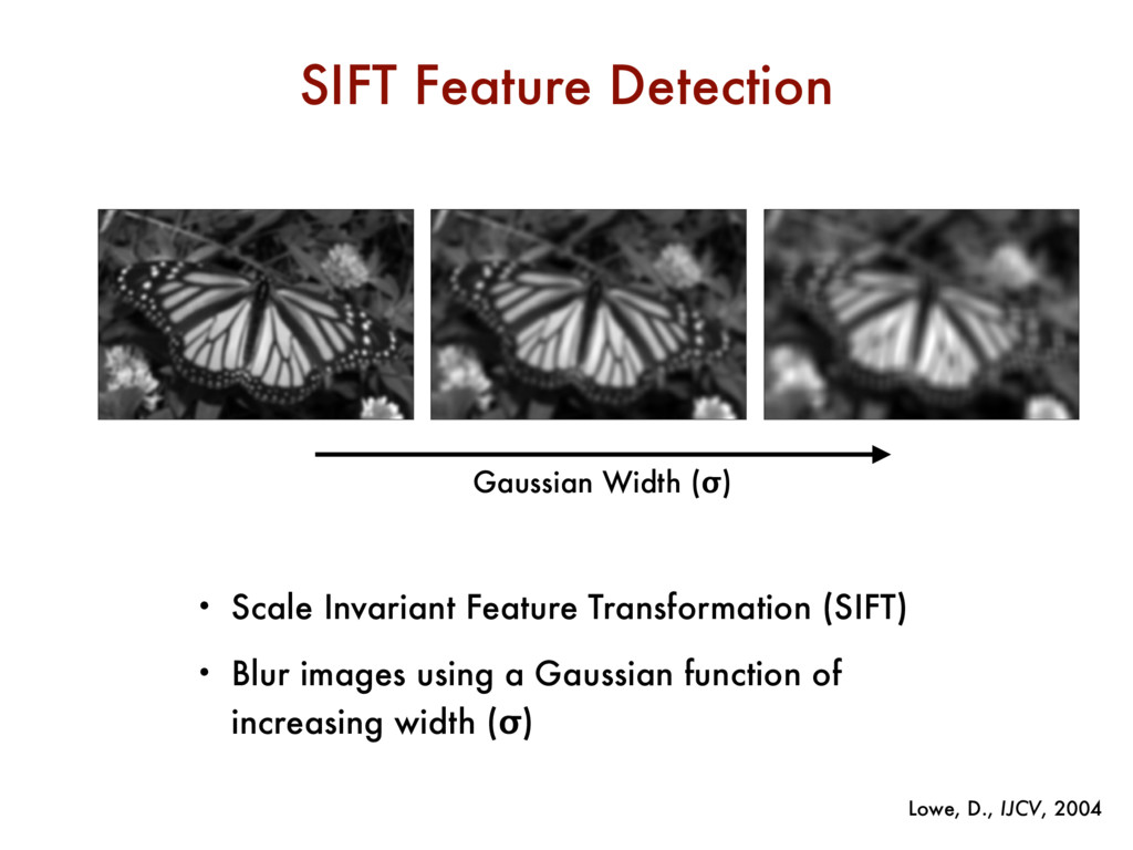
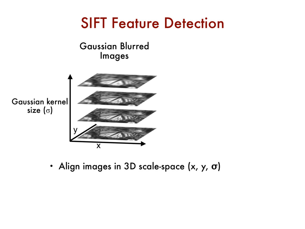
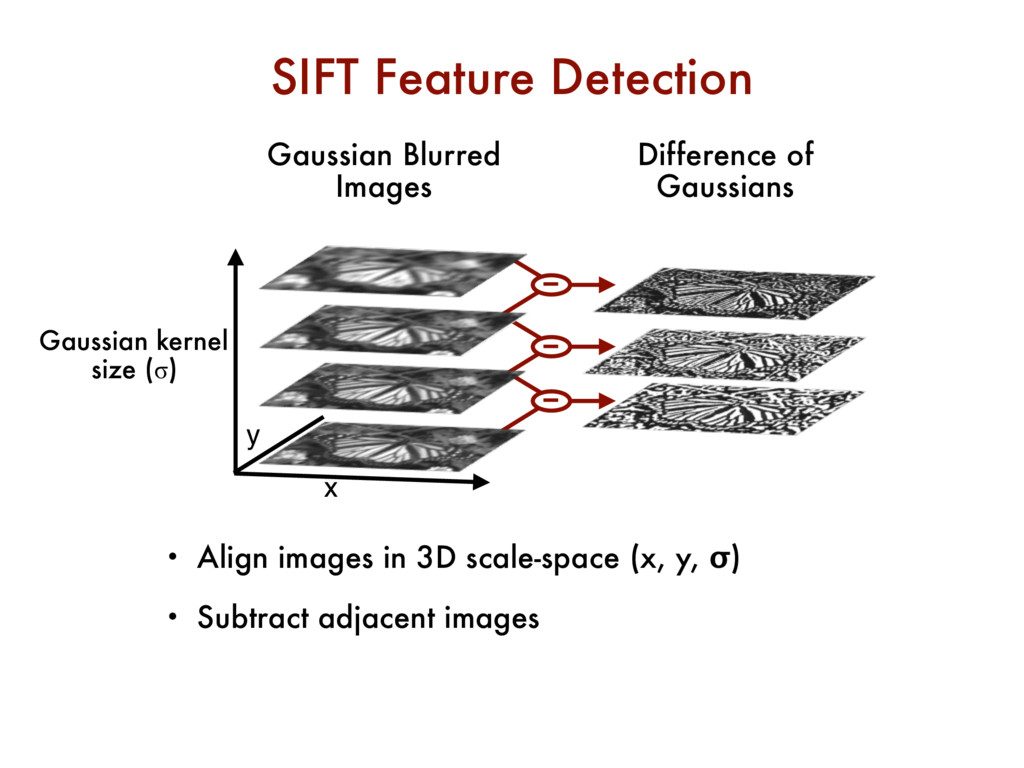
y, σ) • Subtract adjacent images • Local extrema evaluated as potential features x Gaussian Blurred Images Difference of Gaussians Gaussian kernel size (σ) y –
scale-space (x, y, σ) • Subtract adjacent images • Local extrema evaluated as potential features x Gaussian Blurred Images Difference of Gaussians Gaussian kernel size (σ) y –
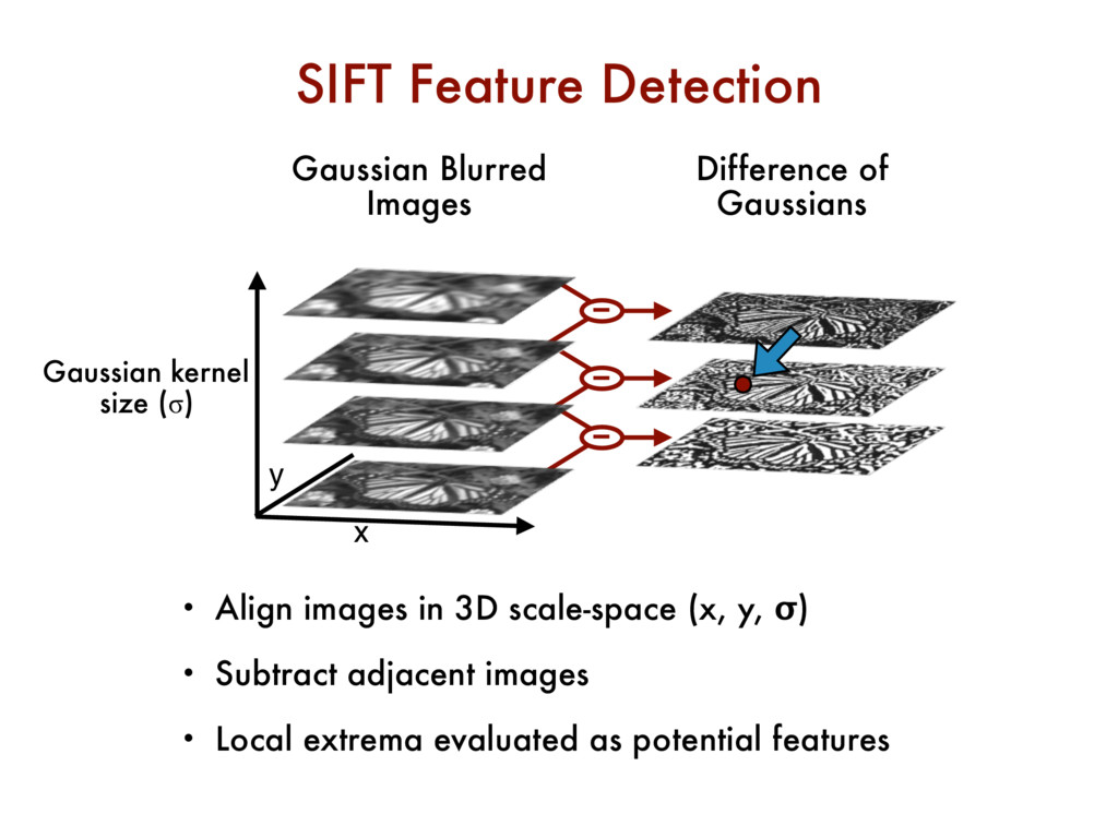
scale-space (x, y, σ) • Subtract adjacent images • Local extrema evaluated as potential features x Gaussian Blurred Images Difference of Gaussians Gaussian kernel size (σ) y –
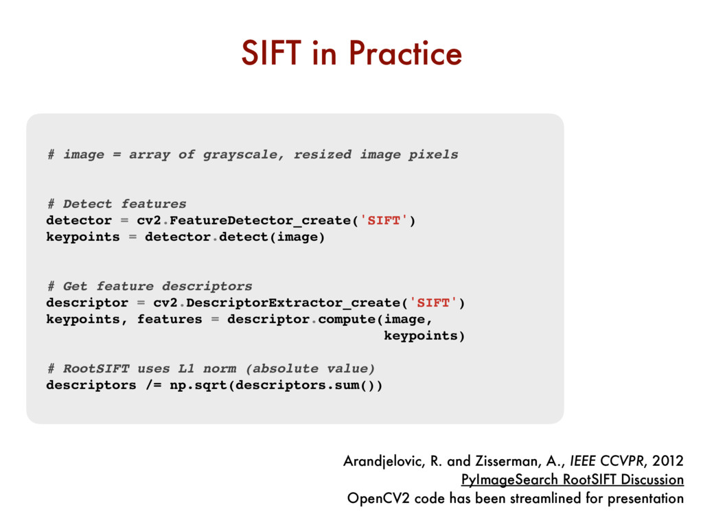
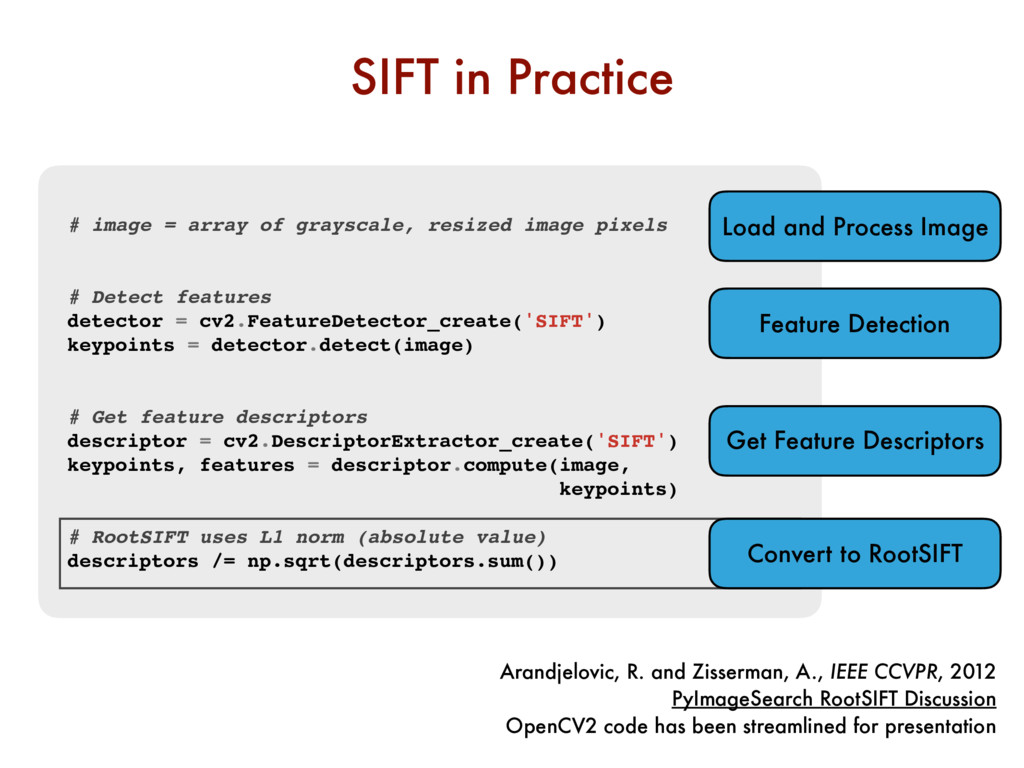
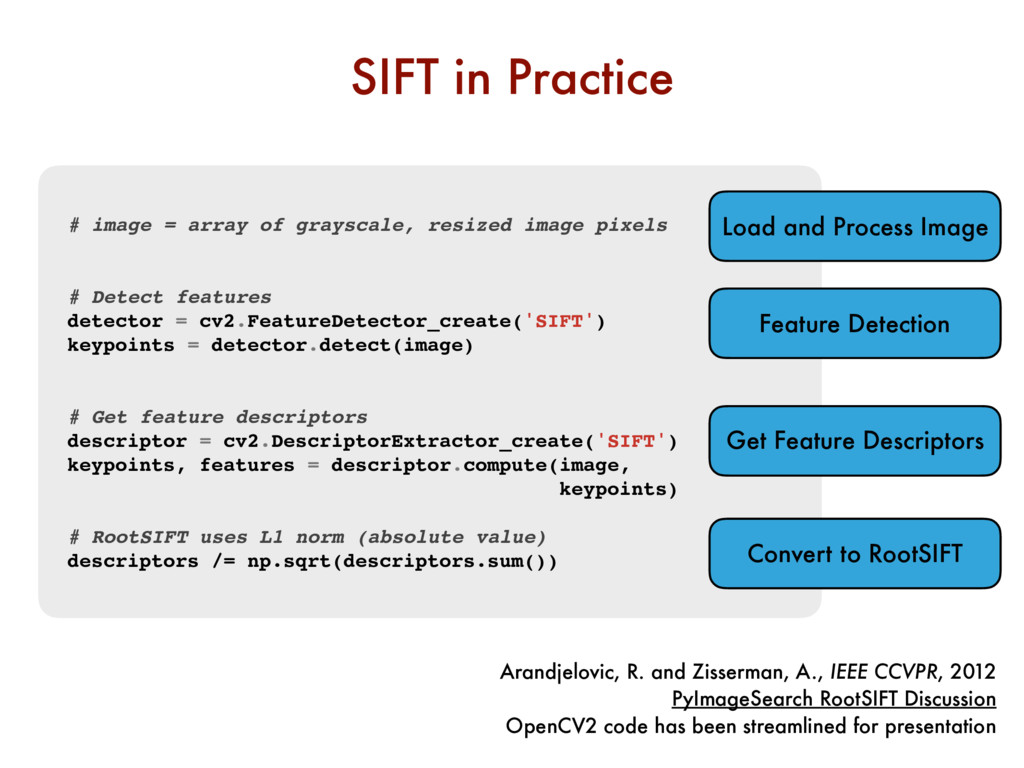
Detect features detector = cv2.FeatureDetector_create('SIFT') keypoints = detector.detect(image) # Get feature descriptors descriptor = cv2.DescriptorExtractor_create('SIFT') keypoints, features = descriptor.compute(image, keypoints) # RootSIFT uses L1 norm (absolute value) descriptors /= np.sqrt(descriptors.sum()) SIFT in Practice Arandjelovic, R. and Zisserman, A., IEEE CCVPR, 2012 PyImageSearch RootSIFT Discussion OpenCV2 code has been streamlined for presentation
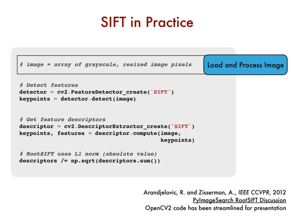
Detect features detector = cv2.FeatureDetector_create('SIFT') keypoints = detector.detect(image) # Get feature descriptors descriptor = cv2.DescriptorExtractor_create('SIFT') keypoints, features = descriptor.compute(image, keypoints) # RootSIFT uses L1 norm (absolute value) descriptors /= np.sqrt(descriptors.sum()) SIFT in Practice Arandjelovic, R. and Zisserman, A., IEEE CCVPR, 2012 PyImageSearch RootSIFT Discussion OpenCV2 code has been streamlined for presentation Load and Process Image
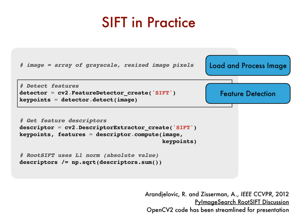
Detect features detector = cv2.FeatureDetector_create('SIFT') keypoints = detector.detect(image) # Get feature descriptors descriptor = cv2.DescriptorExtractor_create('SIFT') keypoints, features = descriptor.compute(image, keypoints) # RootSIFT uses L1 norm (absolute value) descriptors /= np.sqrt(descriptors.sum()) SIFT in Practice Arandjelovic, R. and Zisserman, A., IEEE CCVPR, 2012 PyImageSearch RootSIFT Discussion OpenCV2 code has been streamlined for presentation Load and Process Image Feature Detection
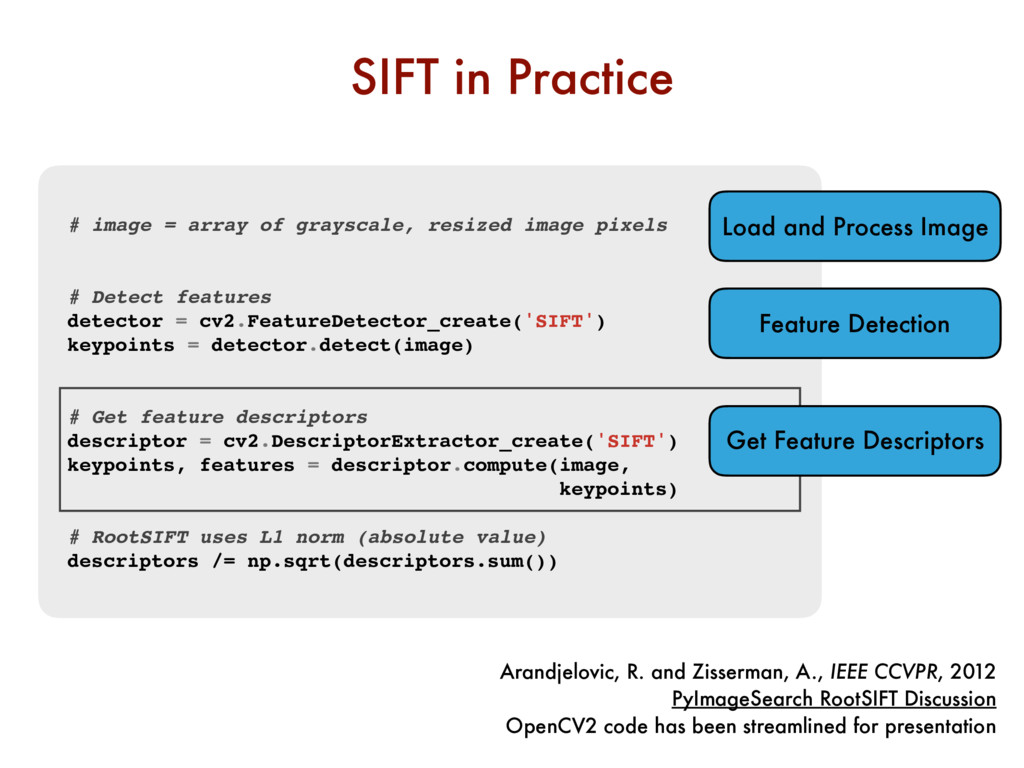
Detect features detector = cv2.FeatureDetector_create('SIFT') keypoints = detector.detect(image) # Get feature descriptors descriptor = cv2.DescriptorExtractor_create('SIFT') keypoints, features = descriptor.compute(image, keypoints) # RootSIFT uses L1 norm (absolute value) descriptors /= np.sqrt(descriptors.sum()) SIFT in Practice Arandjelovic, R. and Zisserman, A., IEEE CCVPR, 2012 PyImageSearch RootSIFT Discussion OpenCV2 code has been streamlined for presentation Load and Process Image Feature Detection Get Feature Descriptors
Detect features detector = cv2.FeatureDetector_create('SIFT') keypoints = detector.detect(image) # Get feature descriptors descriptor = cv2.DescriptorExtractor_create('SIFT') keypoints, features = descriptor.compute(image, keypoints) # RootSIFT uses L1 norm (absolute value) descriptors /= np.sqrt(descriptors.sum()) SIFT in Practice Arandjelovic, R. and Zisserman, A., IEEE CCVPR, 2012 PyImageSearch RootSIFT Discussion OpenCV2 code has been streamlined for presentation Load and Process Image Feature Detection Get Feature Descriptors Convert to RootSIFT
Detect features detector = cv2.FeatureDetector_create('SIFT') keypoints = detector.detect(image) # Get feature descriptors descriptor = cv2.DescriptorExtractor_create('SIFT') keypoints, features = descriptor.compute(image, keypoints) # RootSIFT uses L1 norm (absolute value) descriptors /= np.sqrt(descriptors.sum()) SIFT in Practice Arandjelovic, R. and Zisserman, A., IEEE CCVPR, 2012 PyImageSearch RootSIFT Discussion OpenCV2 code has been streamlined for presentation Load and Process Image Feature Detection Get Feature Descriptors Convert to RootSIFT
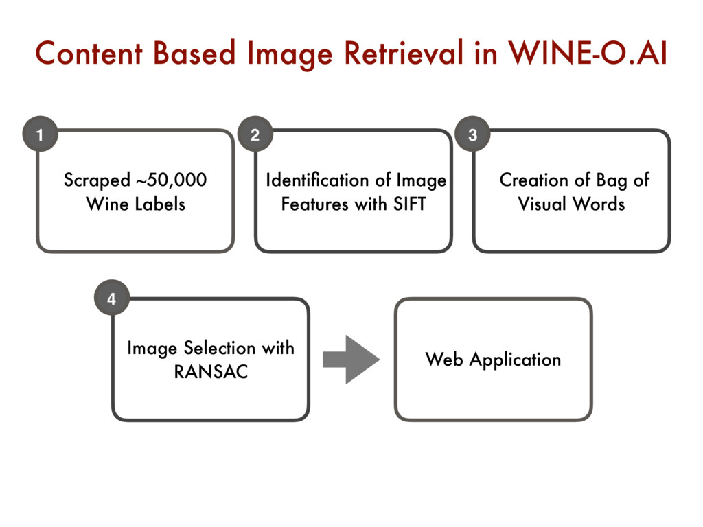
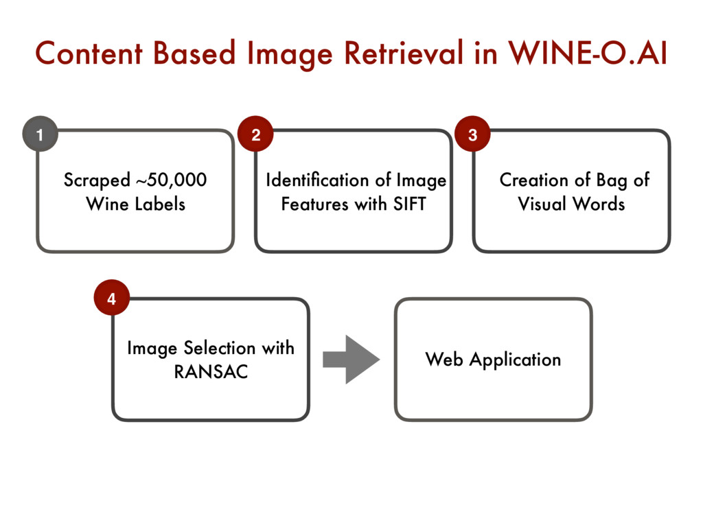
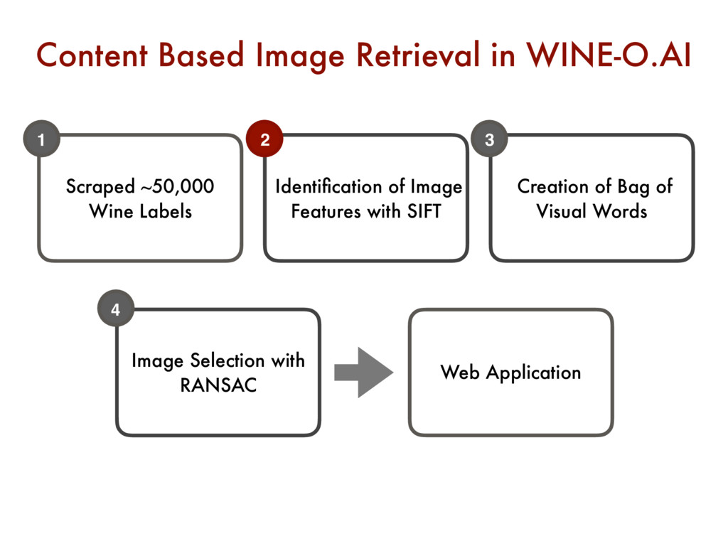
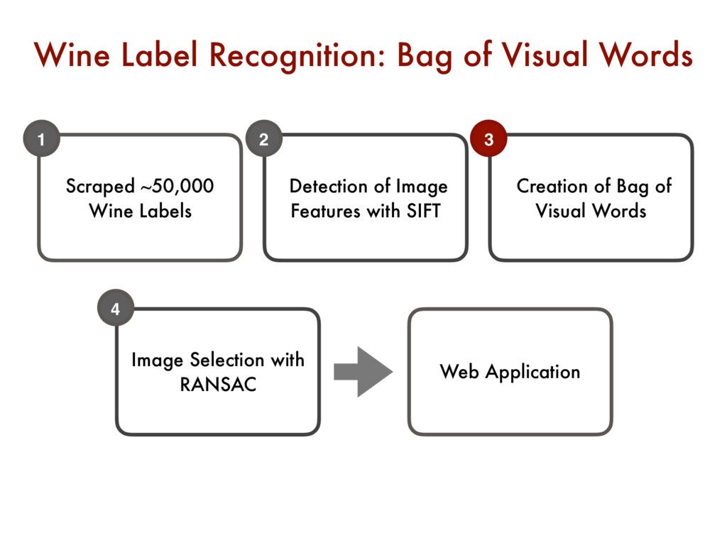
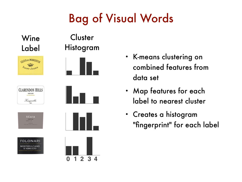
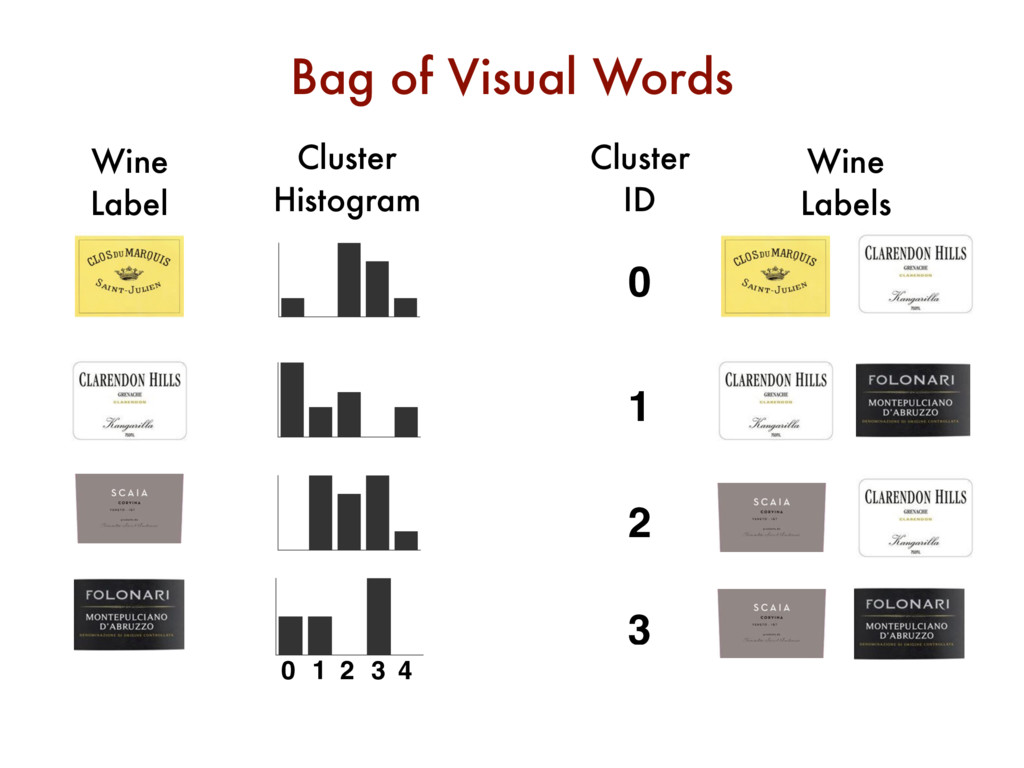
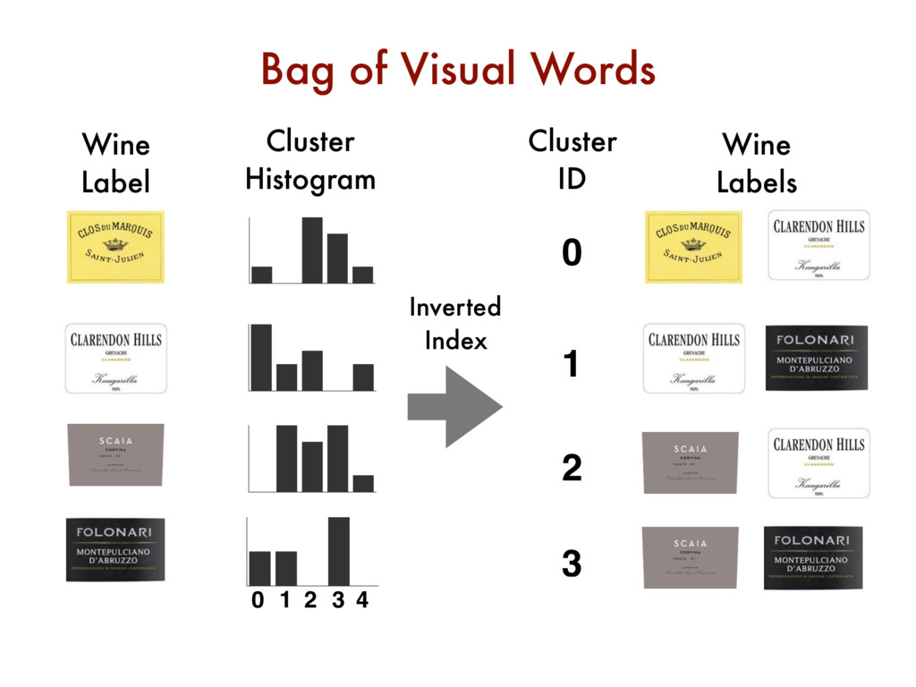
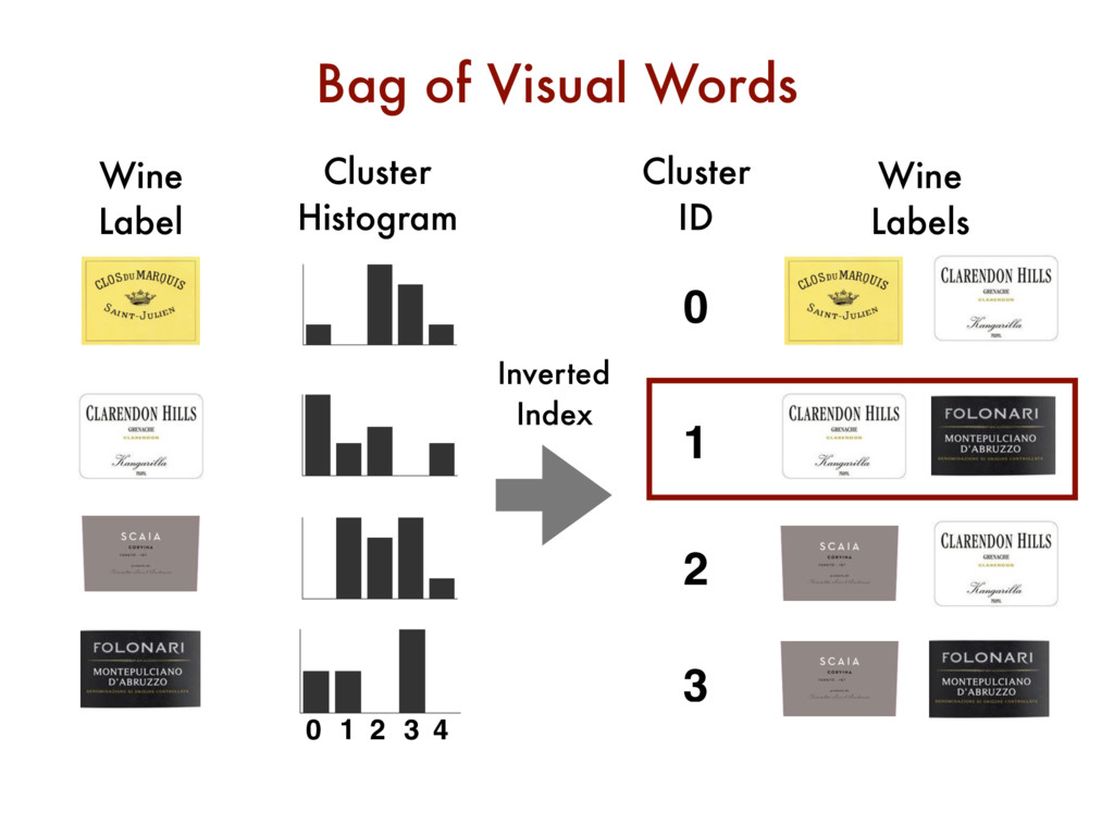
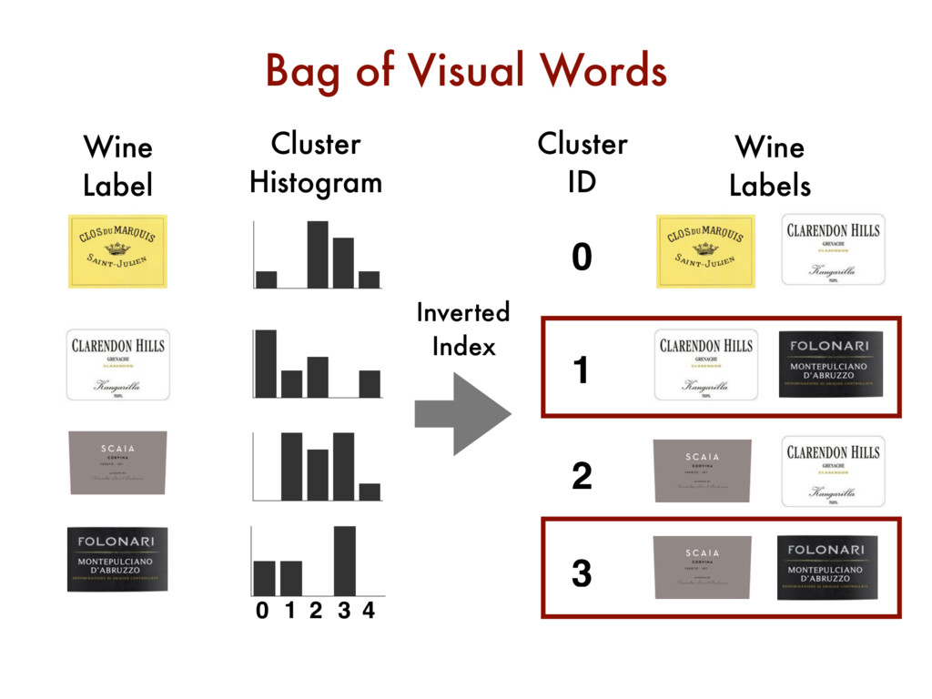
Map features for each label to nearest cluster • Creates a histogram "fingerprint" for each label Bag of Visual Words Wine Label Cluster Histogram 0 1 2 3 4
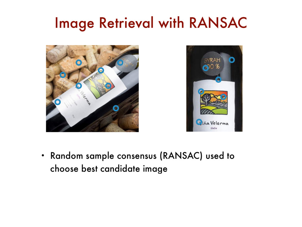
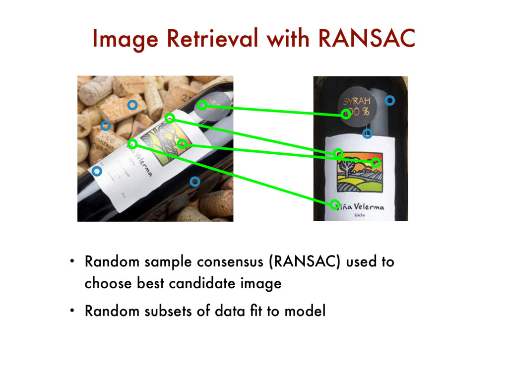
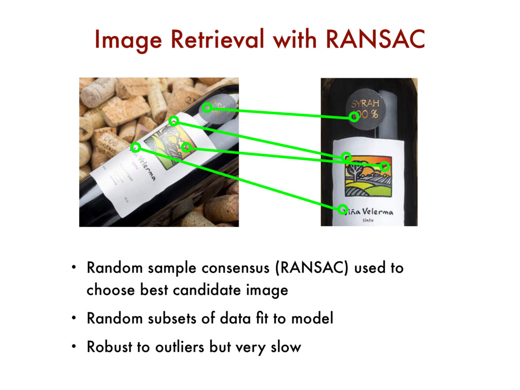
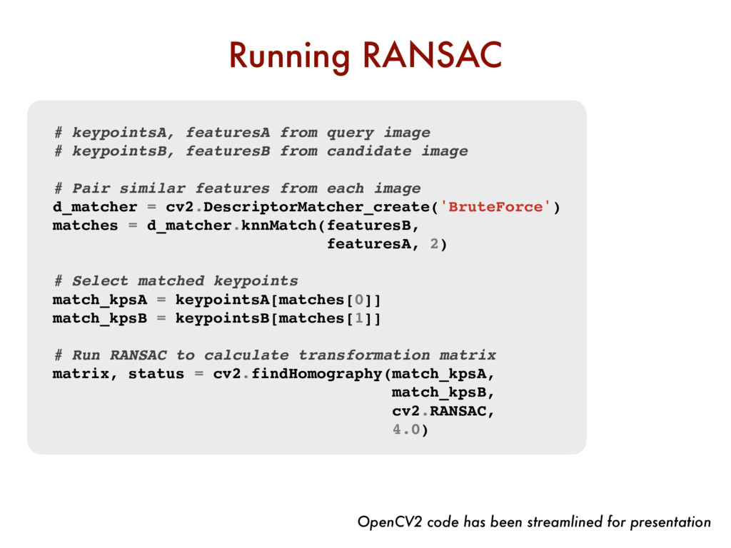
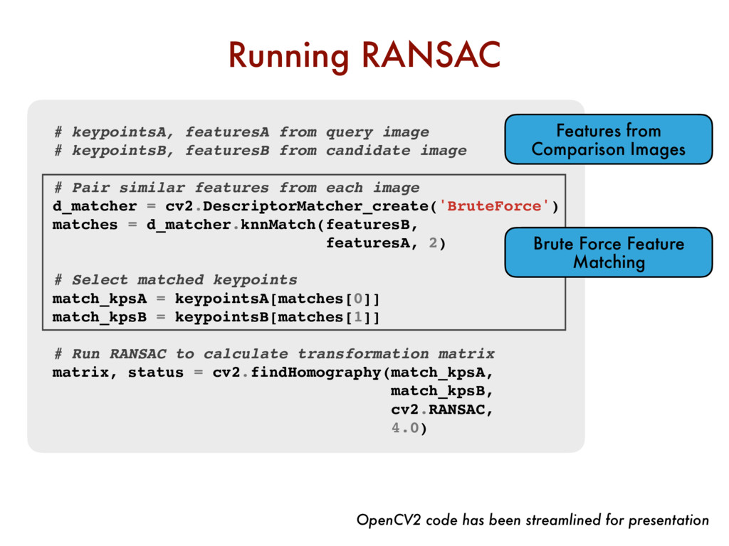
candidate image # Pair similar features from each image d_matcher = cv2.DescriptorMatcher_create('BruteForce') matches = d_matcher.knnMatch(featuresB, featuresA, 2) # Select matched keypoints match_kpsA = keypointsA[matches[0]] match_kpsB = keypointsB[matches[1]] # Run RANSAC to calculate transformation matrix matrix, status = cv2.findHomography(match_kpsA, match_kpsB, cv2.RANSAC, 4.0) Running RANSAC OpenCV2 code has been streamlined for presentation
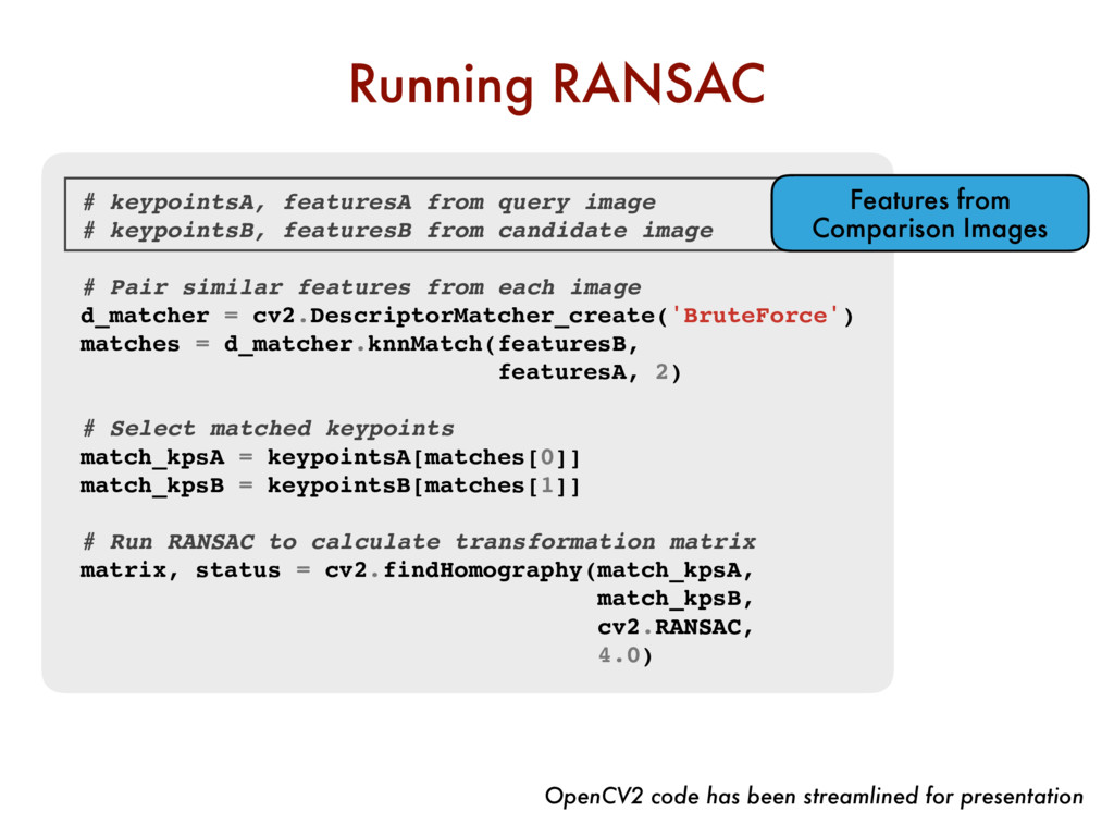
candidate image # Pair similar features from each image d_matcher = cv2.DescriptorMatcher_create('BruteForce') matches = d_matcher.knnMatch(featuresB, featuresA, 2) # Select matched keypoints match_kpsA = keypointsA[matches[0]] match_kpsB = keypointsB[matches[1]] # Run RANSAC to calculate transformation matrix matrix, status = cv2.findHomography(match_kpsA, match_kpsB, cv2.RANSAC, 4.0) Running RANSAC OpenCV2 code has been streamlined for presentation Features from Comparison Images
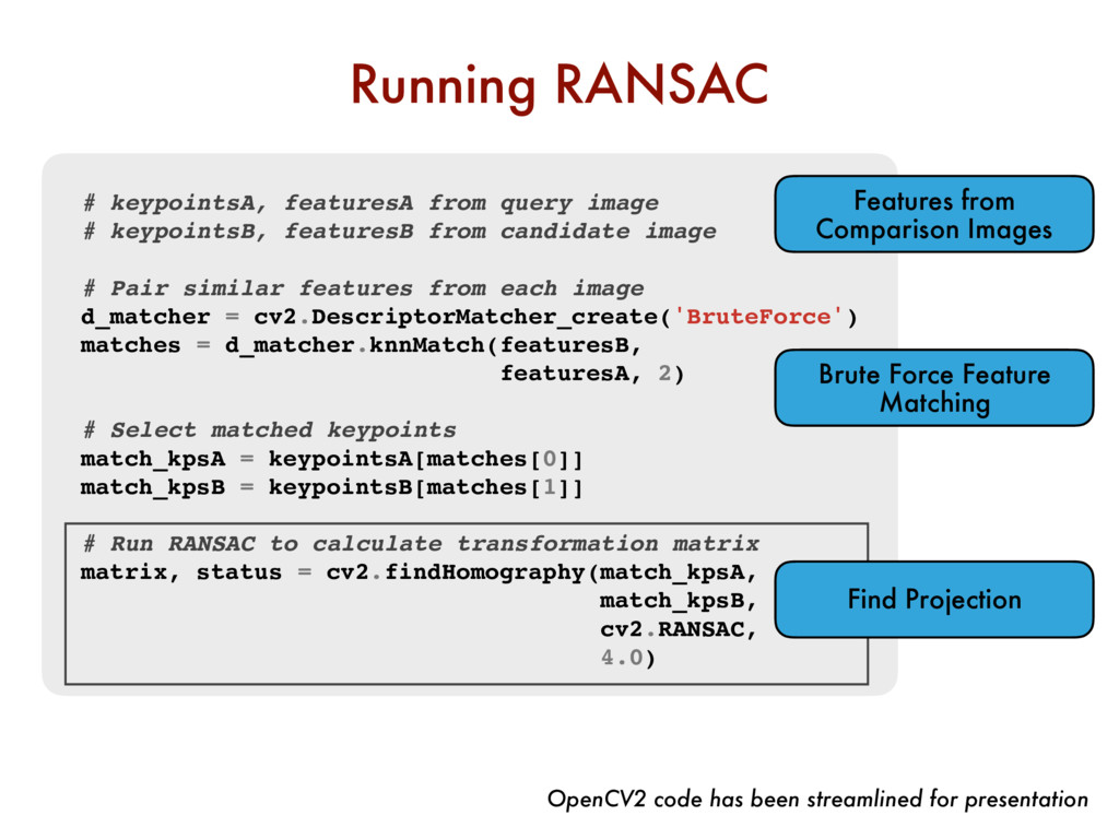
candidate image # Pair similar features from each image d_matcher = cv2.DescriptorMatcher_create('BruteForce') matches = d_matcher.knnMatch(featuresB, featuresA, 2) # Select matched keypoints match_kpsA = keypointsA[matches[0]] match_kpsB = keypointsB[matches[1]] # Run RANSAC to calculate transformation matrix matrix, status = cv2.findHomography(match_kpsA, match_kpsB, cv2.RANSAC, 4.0) Running RANSAC OpenCV2 code has been streamlined for presentation Features from Comparison Images Brute Force Feature Matching
candidate image # Pair similar features from each image d_matcher = cv2.DescriptorMatcher_create('BruteForce') matches = d_matcher.knnMatch(featuresB, featuresA, 2) # Select matched keypoints match_kpsA = keypointsA[matches[0]] match_kpsB = keypointsB[matches[1]] # Run RANSAC to calculate transformation matrix matrix, status = cv2.findHomography(match_kpsA, match_kpsB, cv2.RANSAC, 4.0) Running RANSAC OpenCV2 code has been streamlined for presentation Features from Comparison Images Brute Force Feature Matching Find Projection
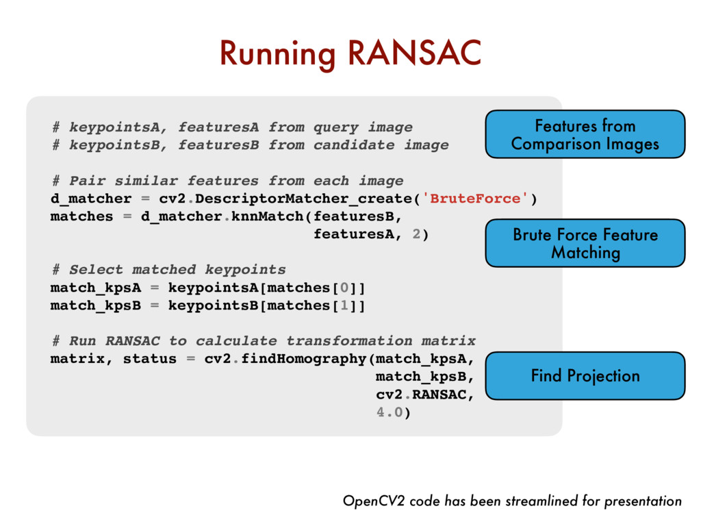
candidate image # Pair similar features from each image d_matcher = cv2.DescriptorMatcher_create('BruteForce') matches = d_matcher.knnMatch(featuresB, featuresA, 2) # Select matched keypoints match_kpsA = keypointsA[matches[0]] match_kpsB = keypointsB[matches[1]] # Run RANSAC to calculate transformation matrix matrix, status = cv2.findHomography(match_kpsA, match_kpsB, cv2.RANSAC, 4.0) Running RANSAC OpenCV2 code has been streamlined for presentation Features from Comparison Images Brute Force Feature Matching Find Projection
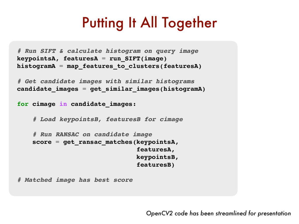
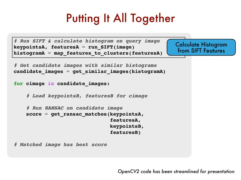
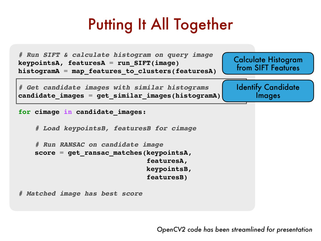
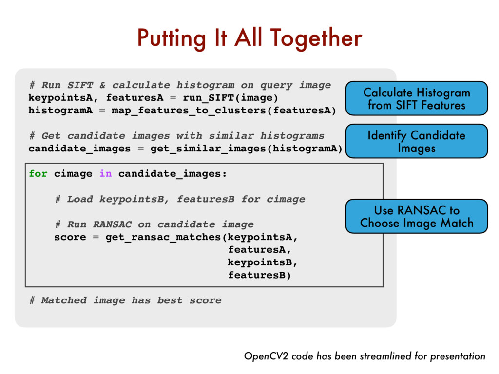
featuresA = run_SIFT(image) histogramA = map_features_to_clusters(featuresA) # Get candidate images with similar histograms candidate_images = get_similar_images(histogramA) for cimage in candidate_images: # Load keypointsB, featuresB for cimage # Run RANSAC on candidate image score = get_ransac_matches(keypointsA, featuresA, keypointsB, featuresB) # Matched image has best score Putting It All Together OpenCV2 code has been streamlined for presentation
featuresA = run_SIFT(image) histogramA = map_features_to_clusters(featuresA) # Get candidate images with similar histograms candidate_images = get_similar_images(histogramA) for cimage in candidate_images: # Load keypointsB, featuresB for cimage # Run RANSAC on candidate image score = get_ransac_matches(keypointsA, featuresA, keypointsB, featuresB) # Matched image has best score Putting It All Together OpenCV2 code has been streamlined for presentation Calculate Histogram from SIFT Features
featuresA = run_SIFT(image) histogramA = map_features_to_clusters(featuresA) # Get candidate images with similar histograms candidate_images = get_similar_images(histogramA) for cimage in candidate_images: # Load keypointsB, featuresB for cimage # Run RANSAC on candidate image score = get_ransac_matches(keypointsA, featuresA, keypointsB, featuresB) # Matched image has best score Putting It All Together OpenCV2 code has been streamlined for presentation Calculate Histogram from SIFT Features Identify Candidate Images
featuresA = run_SIFT(image) histogramA = map_features_to_clusters(featuresA) # Get candidate images with similar histograms candidate_images = get_similar_images(histogramA) for cimage in candidate_images: # Load keypointsB, featuresB for cimage # Run RANSAC on candidate image score = get_ransac_matches(keypointsA, featuresA, keypointsB, featuresB) # Matched image has best score Putting It All Together OpenCV2 code has been streamlined for presentation Calculate Histogram from SIFT Features Identify Candidate Images Use RANSAC to Choose Image Match
featuresA = run_SIFT(image) histogramA = map_features_to_clusters(featuresA) # Get candidate images with similar histograms candidate_images = get_similar_images(histogramA) for cimage in candidate_images: # Load keypointsB, featuresB for cimage # Run RANSAC on candidate image score = get_ransac_matches(keypointsA, featuresA, keypointsB, featuresB) # Matched image has best score Putting It All Together OpenCV2 code has been streamlined for presentation Calculate Histogram from SIFT Features Identify Candidate Images Use RANSAC to Choose Image Match
![! [email protected] " @modernscientist # themodernscientist $ mlgill Thank You](https://files.speakerdeck.com/presentations/273b632d1be245608b5183210470a7ec/slide_56.jpg)