Chance constrained optimization of a three-stage launcher

by A. Sassi

Transcript

1. Introduction Model Optimization problem Results Conclusions Chance constrained optimization of a three-stage launcher Achille Sassi1 Jean-Baptiste Caillau2, Max Cerf3, Emmanuel Tr´ elat4, Hasnaa Zidani1 1ENSTA ParisTech 2Universit´ e de Bourgogne 3Airbus Defence and Space 4Universit´ e Pierre et Marie Curie Journ´ ees du GdR MOA - Dijon, 02/11/2015
2. Introduction Model Optimization problem Results Conclusions Introduction
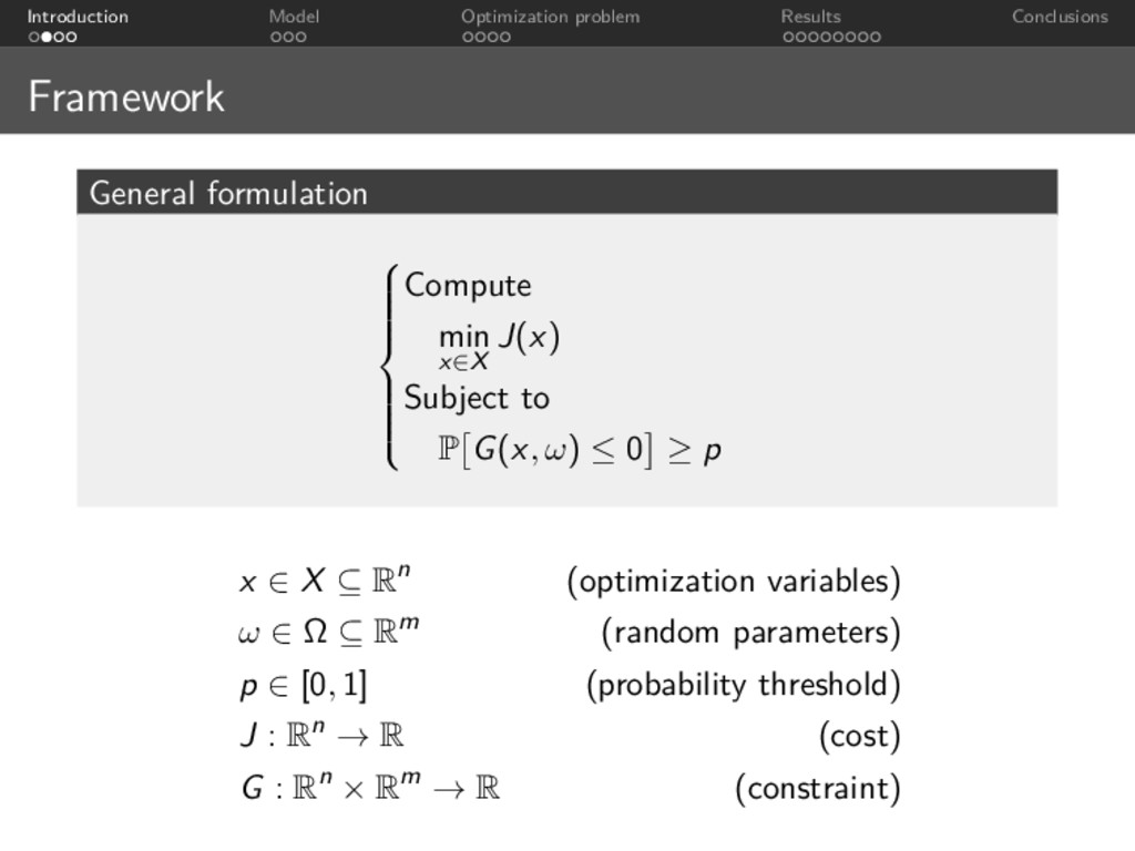
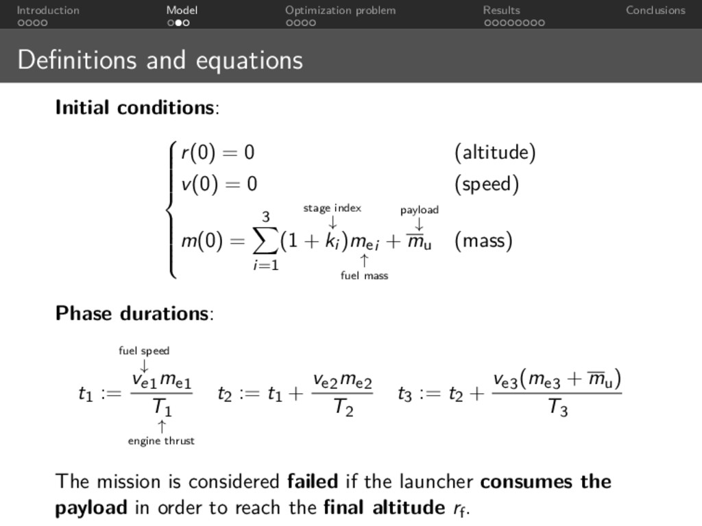
3. Introduction Model Optimization problem Results Conclusions Problem Deliver a payload to a given altitude while minimizing the fuel load of the launcher. Some parameters are subject to uncertainties and we need the mission to succeed with a 90% probability.
4. Introduction Model Optimization problem Results Conclusions Framework General formulation              Compute min x∈X J(x) Subject to P G(x, ω) ≤ 0 ≥ p x ∈ X ⊆ Rn (optimization variables) ω ∈ Ω ⊆ Rm (random parameters) p ∈ [0, 1] (probability threshold) J : Rn → R (cost) G : Rn × Rm → R (constraint)
5. Introduction Model Optimization problem Results Conclusions Approach Problem: for every x in X, the distribution of G(x, ω) is unknown. Solution: approximate it and translate the stochastic optimization problem into a deterministic one: P G(x, ω) ≤ 0 = 0 −∞ fG(x) (ξ)dξ ≈ 0 −∞ ˆ fG(x) (ξ)dξ where fG is the probability density function of G and ˆ fG its approximation.
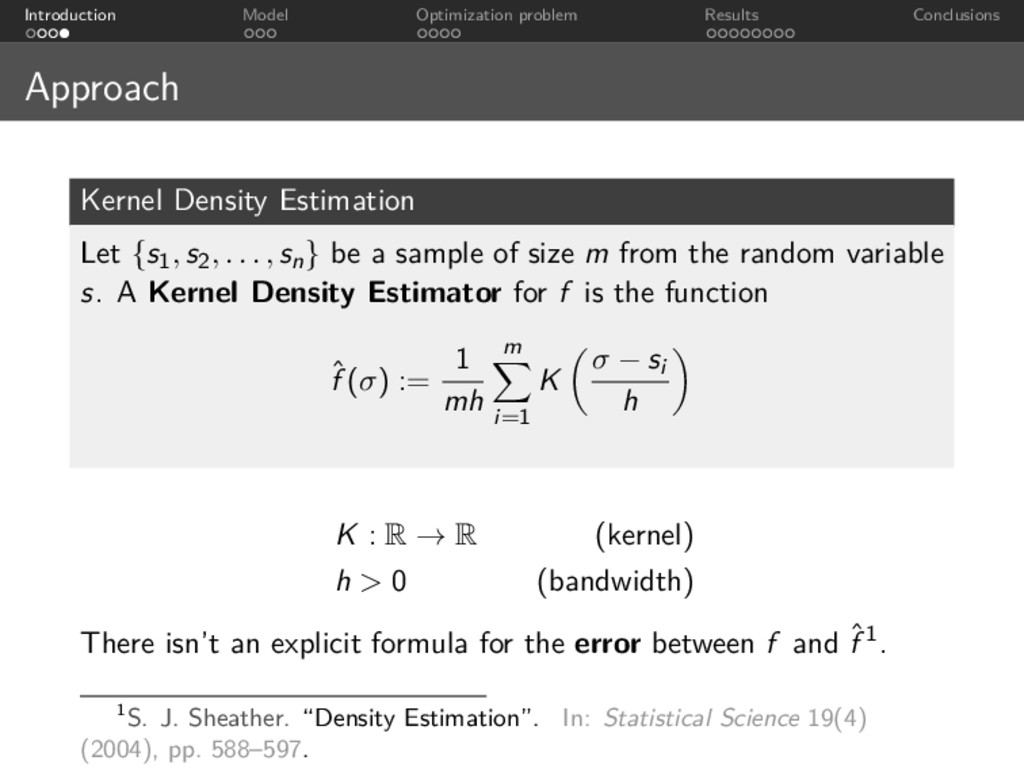
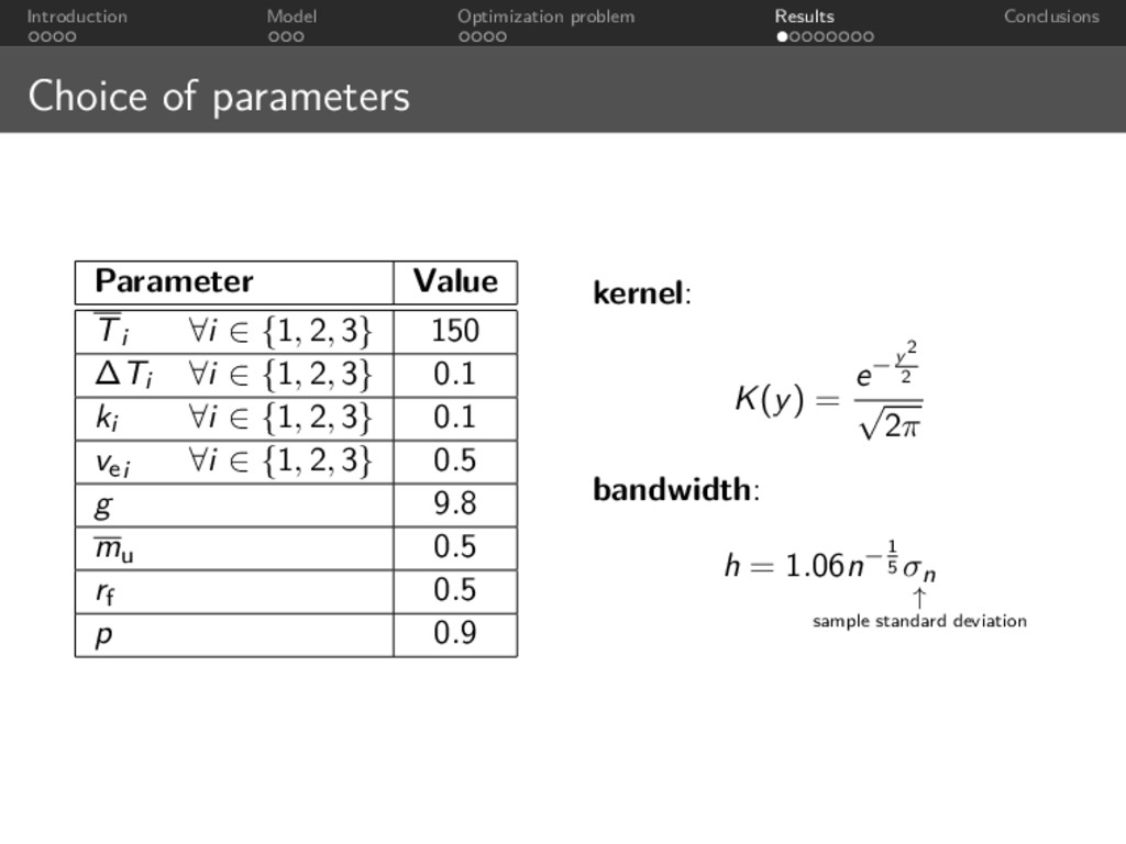
6. Introduction Model Optimization problem Results Conclusions Approach Kernel Density Estimation Let {s1, s2, . . . , sn} be a sample of size m from the random variable s. A Kernel Density Estimator for f is the function ˆ f (σ) := 1 mh m i=1 K σ − si h K : R → R (kernel) h > 0 (bandwidth) There isn’t an explicit formula for the error between f and ˆ f 1. 1S. J. Sheather. “Density Estimation”. In: Statistical Science 19(4) (2004), pp. 588–597.
7. Introduction Model Optimization problem Results Conclusions Model
8. Introduction Model Optimization problem Results Conclusions Description Three-stage launcher = 3 × segment engine+fuel load+structure +payload Flight phases: 1 first stage’s engine ignited until fuel exhaustion; 2 first stage’s structure detached, second stage’s engine ignited until fuel exhaustion; 3 second stage’s structure detached, third stage’s engine ignited until fuel exhaustion; 4 third stage’s structure detached, payload delivered at final altitude.
9. Introduction Model Optimization problem Results Conclusions Definitions and equations Initial conditions:                r(0) = 0 (altitude) v(0) = 0 (speed) m(0) = 3 i=1 (1 + stage index ↓ ki )mei ↑ fuel mass + payload ↓ mu (mass) Phase durations: t1 := fuel speed ↓ ve1 me1 T1 ↑ engine thrust t2 := t1 + ve2 me2 T2 t3 := t2 + ve3 (me3 + mu) T3 The mission is considered failed if the launcher consumes the payload in order to reach the final altitude rf.
10. Introduction Model Optimization problem Results Conclusions Definitions and equations State equation of the i-th phase:            ˙ r(t) = v(t) ˙ v(t) = Ti m(t) − gravitational acceleration ↓ g ˙ m(t) = − Ti vei ∀i ∈ {1, 2, 3} Mass discontinuities between phases: m(ti ) = m(t− i ) − ki mei stage structure ∀i ∈ {1, 2, 3} Random parameters:        Ti ∼ U Ti (1 − ∆Ti ), Ti (1 + ∆Ti )Ii Ii E[Ti ] = Ti ∀i ∈ {1, 2, 3}
11. Introduction Model Optimization problem Results Conclusions Optimization problem
12. Introduction Model Optimization problem Results Conclusions Stochastic optimization problem Case study formulation                  Compute min me∈R3 + 3 i=1 (1 + ki )mei Subject to P Mu(T, me) ≥ mu ≥ p me := (me1 , me2 , me3 ) ∈ R3 + (optimization variables) T := (T1, T2, T3) ∈ I1 × I2 × I3 (random parameters) Mu(T, me) := m t3(T, me) (constraint) For me and T given, t3(T, me) solves r(t3) = rf.
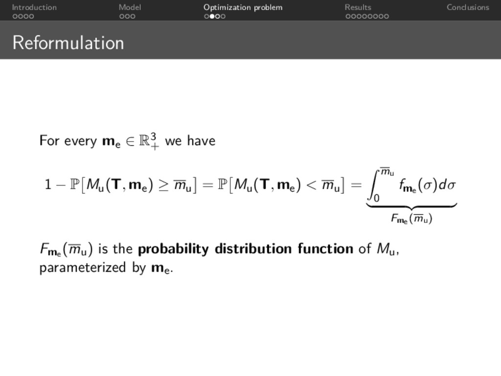
13. Introduction Model Optimization problem Results Conclusions Reformulation For every me ∈ R3 + we have 1 − P Mu(T, me) ≥ mu = P Mu(T, me) < mu = mu 0 fme (σ)dσ Fme (mu) Fme (mu) is the probability distribution function of Mu, parameterized by me.
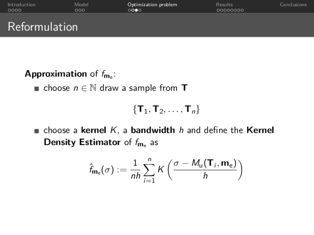
14. Introduction Model Optimization problem Results Conclusions Reformulation Approximation of fme : choose n ∈ N draw a sample from T {T1, T2, . . . , Tn} choose a kernel K, a bandwidth h and define the Kernel Density Estimator of fme as ˆ fme (σ) := 1 nh n i=1 K σ − Mu(Ti , me) h
15. Introduction Model Optimization problem Results Conclusions Deterministic optimization problem Deterministic reformulation                  Compute min me∈R3 + 3 i=1 (1 + ki )mei Subject to ˆ Fme (mu) ≤ 1 − p ˆ Fme (mu) := mu 0 ˆ fme (σ)dσ ≈ mu 0 fme (σ)dσ =: Fme (mu)
16. Introduction Model Optimization problem Results Conclusions Results
17. Introduction Model Optimization problem Results Conclusions Choice of parameters Parameter Value Ti ∀i ∈ {1, 2, 3} 150 ∆Ti ∀i ∈ {1, 2, 3} 0.1 ki ∀i ∈ {1, 2, 3} 0.1 vei ∀i ∈ {1, 2, 3} 0.5 g 9.8 mu 0.5 rf 0.5 p 0.9 kernel: K(y) = e−y2 2 √ 2π bandwidth: h = 1.06n−1 5 σn ↑ sample standard deviation
18. Introduction Model Optimization problem Results Conclusions Test 1: optimal solution For n = 203 we take a uniform sample from T ∈ I1 × I2 × I3, and compute the optimal solution me1 ≈2.80326 me2 ≈1.88891 me3 ≈1.56716 which allows us to deliver the payload with a probability of 91,7% even if the maximum thrust Ti of each engine is subject to random oscillations.
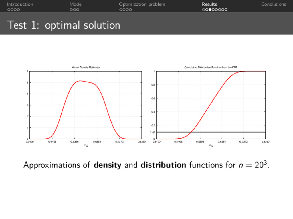
19. Introduction Model Optimization problem Results Conclusions Test 1: optimal solution 0 1 2 3 4 5 6 0.3420 0.4408 0.5396 0.6384 0.7372 0.8360 mu Kernel Density Estimator 0 0.2 0.4 0.6 0.8 1 0.3420 0.4408 0.5396 0.6384 0.7372 0.8360 mu Cumulative Distribution Function from the KDE 1 - p Approximations of density and distribution functions for n = 203.
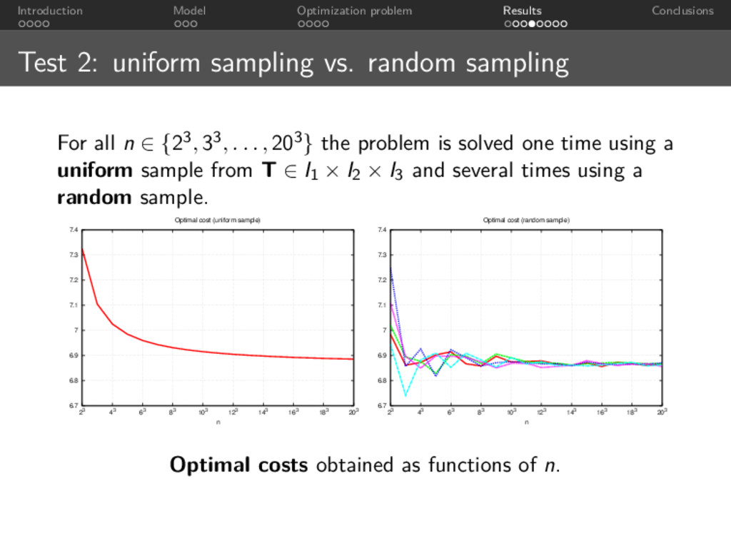
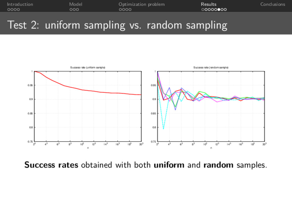
20. Introduction Model Optimization problem Results Conclusions Test 2: uniform sampling vs. random sampling For all n ∈ {23, 33, . . . , 203} the problem is solved one time using a uniform sample from T ∈ I1 × I2 × I3 and several times using a random sample. 6.7 6.8 6.9 7 7.1 7.2 7.3 7.4 23 43 63 83 103 123 143 163 183 203 n Optimal cost (uniform sample) 6.7 6.8 6.9 7 7.1 7.2 7.3 7.4 23 43 63 83 103 123 143 163 183 203 n Optimal cost (random sample) Optimal costs obtained as functions of n.
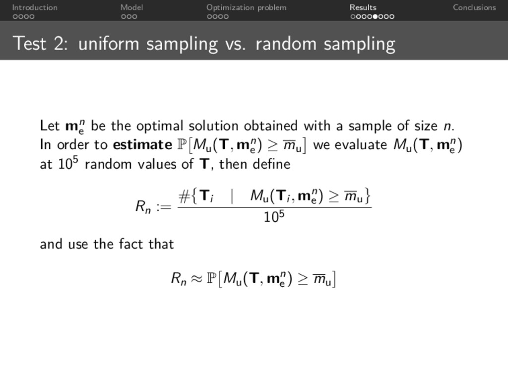
21. Introduction Model Optimization problem Results Conclusions Test 2: uniform sampling vs. random sampling Let mn e be the optimal solution obtained with a sample of size n. In order to estimate P Mu(T, mn e ) ≥ mu we evaluate Mu(T, mn e ) at 105 random values of T, then define Rn := # Ti | Mu(Ti , mn e ) ≥ mu 105 and use the fact that Rn ≈ P Mu(T, mn e ) ≥ mu
22. Introduction Model Optimization problem Results Conclusions Test 2: uniform sampling vs. random sampling 0.75 0.8 0.85 0.9 0.95 1 23 43 63 83 103 123 143 163 183 203 n Success rate (uniform sample) 0.75 0.8 0.85 0.9 0.95 1 23 43 63 83 103 123 143 163 183 203 n Success rate (random sample) Success rates obtained with both uniform and random samples.
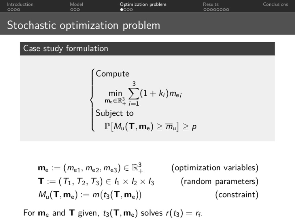
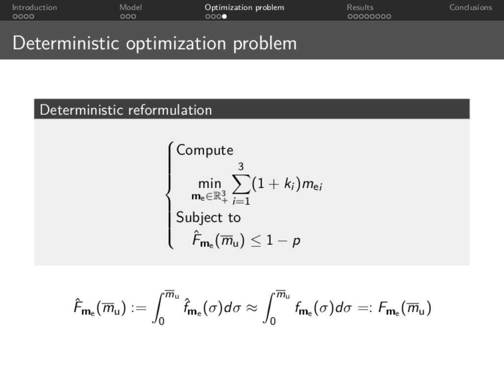
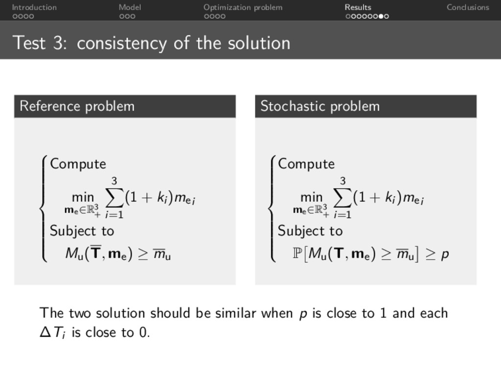
23. Introduction Model Optimization problem Results Conclusions Test 3: consistency of the solution Reference problem                  Compute min me∈R3 + 3 i=1 (1 + ki )mei Subject to Mu(T, me) ≥ mu Stochastic problem                  Compute min me∈R3 + 3 i=1 (1 + ki )mei Subject to P Mu(T, me) ≥ mu ≥ p The two solution should be similar when p is close to 1 and each ∆Ti is close to 0.
24. Introduction Model Optimization problem Results Conclusions Test 3: consistency of the solution n p ∆Ti me1 me2 me3 Stochastic 203 0.9 0.1 2.89042 2.00679 1.62627 203 0.9 0.01 2.70905 1.72067 1.52013 203 0.9 0.001 2.68444 1.70864 1.51171 203 0.9 0.0001 2.68280 1.70825 1.51196 203 0.9 0.00001 2.68279 1.70823 1.51198 Reference N.A. 2.67096 1.73646 1.48640
25. Introduction Model Optimization problem Results Conclusions Conclusions
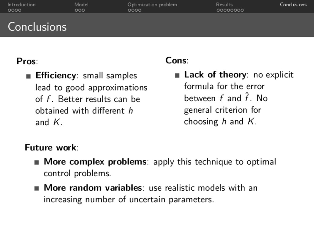
26. Introduction Model Optimization problem Results Conclusions Conclusions Pros: Efficiency: small samples lead to good approximations of f . Better results can be obtained with different h and K. Cons: Lack of theory: no explicit formula for the error between f and ˆ f . No general criterion for choosing h and K. Future work: More complex problems: apply this technique to optimal control problems. More random variables: use realistic models with an increasing number of uncertain parameters.
27. Introduction Model Optimization problem Results Conclusions Fin