Improving the Representation of Major Landforms in Analytical Relief Shading

Brooke Marston
Bernhard Jenny
Oregon State University
#nacis2015

Transcript

1. Improving the Representation of Major
   Landforms in Analytical Relief Shading
   Brooke Marston
   Bernhard Jenny
   NACIS Minneapolis
   October 14–17, 2015
   

   View Slide

2. Relief Shading
   Analytical Manual
   Source: shadedreliefarchive.com
   

   View Slide

3. Adjustment to Illumination Direction
   Global Local
   

   View Slide

4. Why is manual preferred?
   • Locally bright and dark slopes improve legibility
   • Easier and faster to interpret topography
   • Better for small-scale maps where contours degenerate
   Source: shadedreliefarchive.com
   

   View Slide

5. Why aren`t there more manually

   View Slide

6. Benefits of Automation
   • Faster production of shaded relief adhering to manual
   design principles
   • More aesthetically pleasing maps
   • Explicit terrain visualization
   • Improve quality of maps produced by non-professionals
   

   View Slide

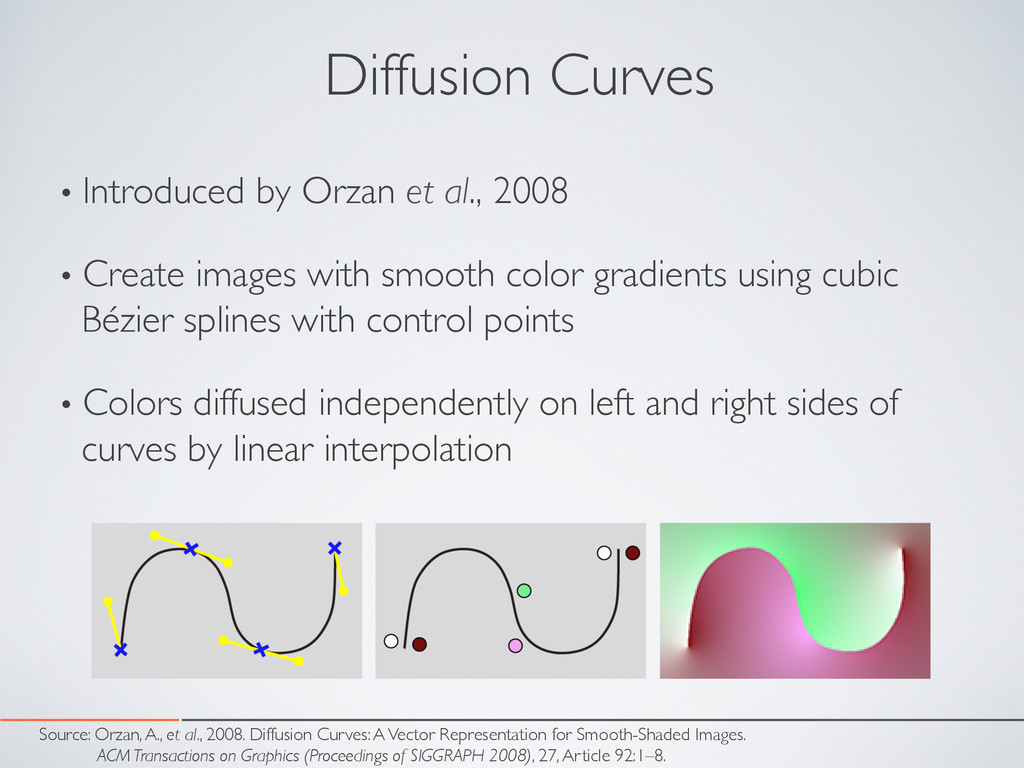
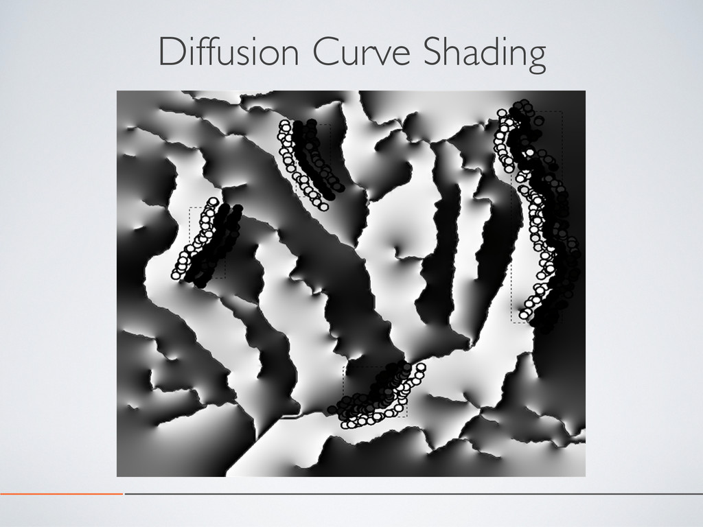
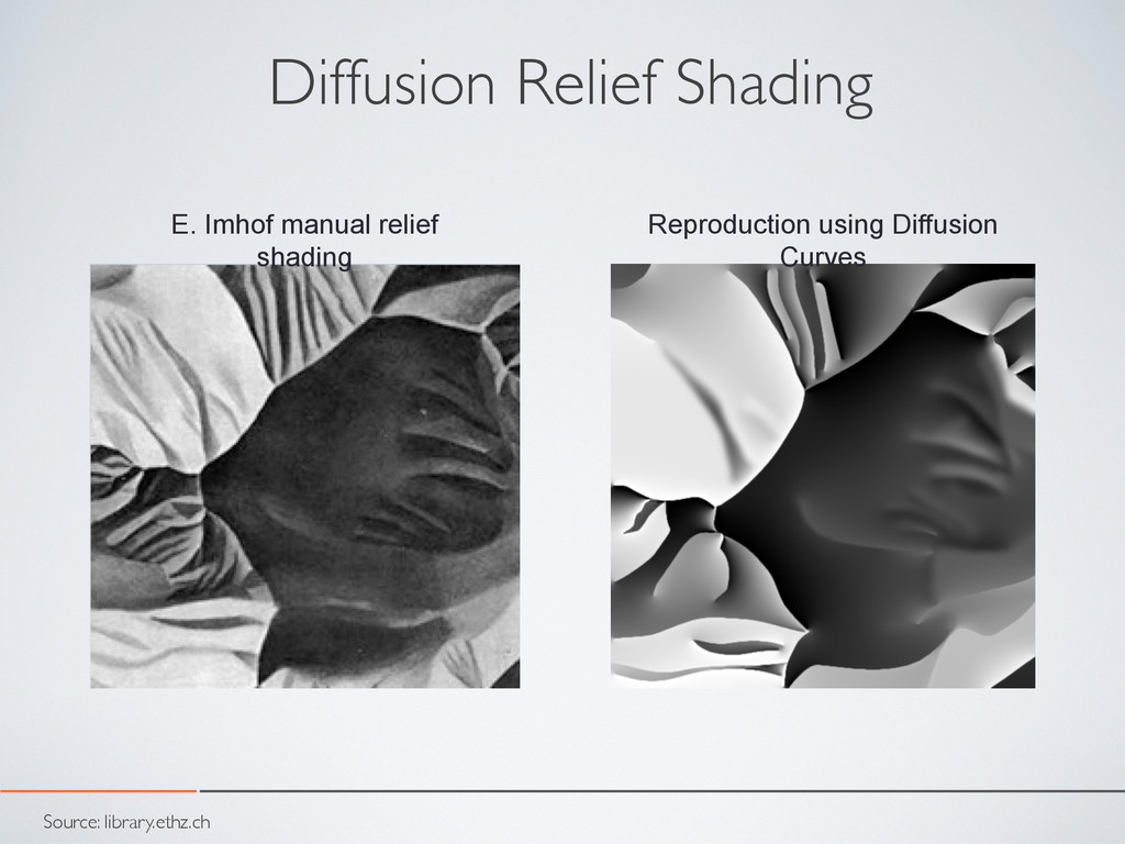
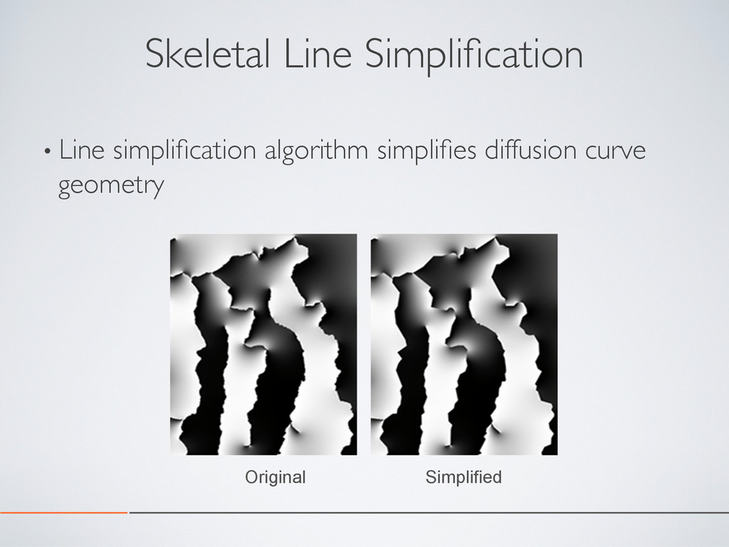
7. Source: Orzan, A., et al., 2008. Diffusion Curves: A Vector Representation for Smooth-Shaded Images.
   ACM Transactions on Graphics (Proceedings of SIGGRAPH 2008), 27, Article 92:1–8.
   Diffusion Curves
   • Introduced by Orzan et al., 2008
   • Create images with smooth color gradients using cubic
   Bézier splines with control points
   • Colors diffused independently on left and right sides of
   curves by linear interpolation
   

   View Slide

8. Ridgelines Valley lines
   Diffusion curve shading
   

   View Slide

9. Identifying valley lines

   View Slide

10. Identifying ridgelines

    View Slide

11. Terrain Tilting
    •  Wedge-shaped base with artificial elevation grade (γ) applied
    to terrain model 8 times (N, E, S, W, NE, NW, SE, SW)
    •  Ridgelines are filtered based on their stability
    

    View Slide

12. Extracting Skeletal Lines
    Flow accumulation Maximum branch
    length
    Ridgeline and valley
    line vectors
    

    View Slide

13. Illumination Adjustment

    View Slide

14. Illumination Adjustment

    View Slide

15. Aspect Simplification
    • Reduces variability of adjusted illumination directions
    • Results in more regular gray values along ridges and valleys
    Original
    Low
    tolerance
    High
    tolerance
    

    View Slide

16. Diffusion Curve Shading
    

    View Slide

17. Valley Floor Mask
    • Detected using seed fill algorithm
    • Visually connects adjacent mountain slopes
    Seed points Valley floor
    

    View Slide

18. Standard analytical
    shading
    Diffusion Relief Shading
    Diffusion curve shading
    Valley floor mask
    + +
    

    View Slide

19. Study Sites
    1.  Alpine terrain
    2.  Pre-alpine terrain
    3.  Terrain with complex drainage network
    

    View Slide

20. 1. Alpine Terrain
    Analytical Diffusion relief shading
    DEM Source: Federal Office of Topography swisstopo
    

    View Slide

21. 1. Alpine Terrain
    Manual Diffusion relief shading
    DEM Source: Federal Office of Topography swisstopo
    

    View Slide

22. 2. Pre-alpine Terrain
    Analytical Diffusion relief shading
    DEM Source: Federal Office of Topography swisstopo
    

    View Slide

23. 3. Complex Drainage Network
    Analytical Diffusion relief shading
    DEM Source: USGS
    

    View Slide

24. Limitations
    • Runtime
    • Spatial extent of terrain model
    • Unwanted artifacts in valley floor mask
    

    View Slide

25. Conclusions
    • Diffusion curve shading enhanced analytical shading
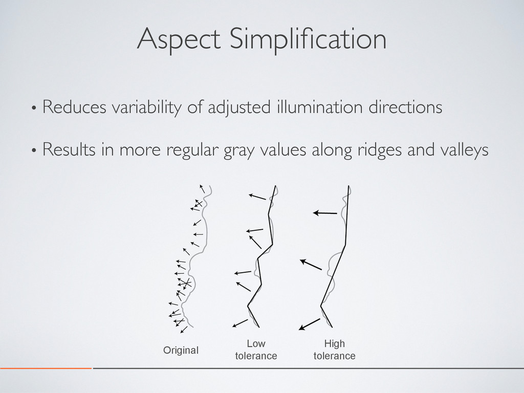
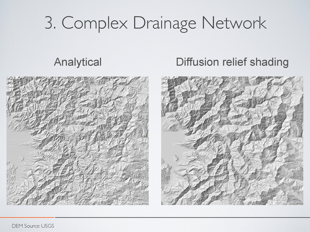
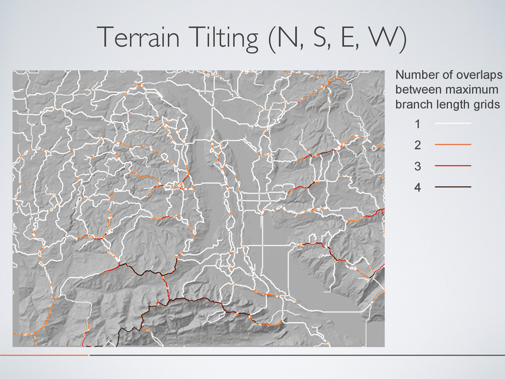
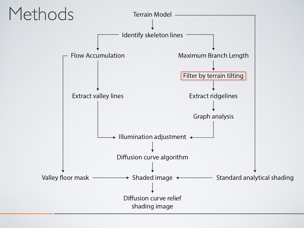
    • Best results in terrain with sharp, clearly defined ridges
    and valleys
    • Tilting removes irrelevant or visually disturbing ridgelines
    • Our method presents alternative to other filter-based
    generalization approaches
    

    View Slide

26. Future Work
    • Incorporate colors modulated by elevation and
    exposure to illumination (Jenny and Hurni 2006)
    • Integrate software applications
    

    View Slide

27. Acknowledgments
    •  Tom Patterson, National Park Service
    •  OSU Cartography and Geovisualization Group
    •  Oregon State University, AAG Cartography Specialty Group,
    Google, ICA Commission on Mountain Cartography, Phi Beta
    Kappa
    

    View Slide

28. Thank you
    Questions?
    

    View Slide

29. Gray value = 255 × cos(α)
    Analytical Relief Shading
    Lambert Shading Algorithm
    

    View Slide

30. Why is manual preferred?
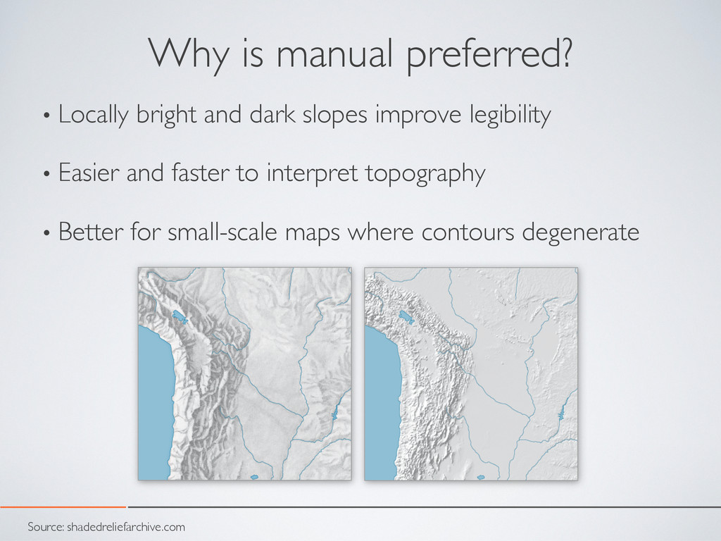
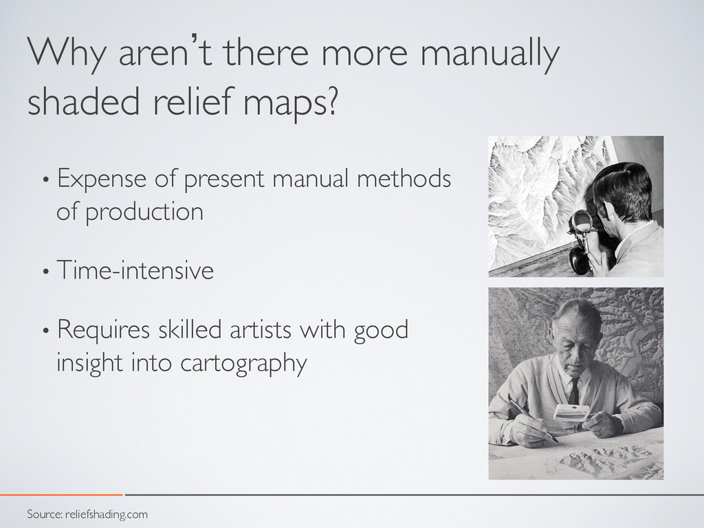
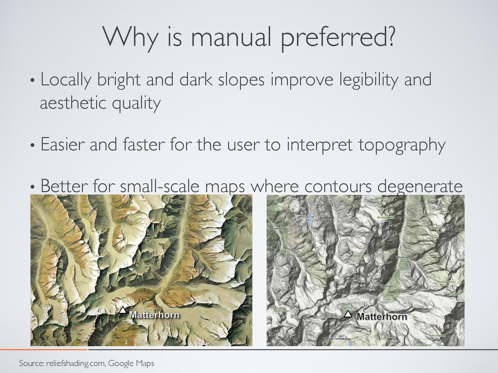
    • Locally bright and dark slopes improve legibility and
    aesthetic quality
    • Easier and faster for the user to interpret topography
    • Better for small-scale maps where contours degenerate
    Source: reliefshading.com, Google Maps
    

    View Slide

31. Why is manual preferred?
    • Better for small-scale maps where contours degenerate
    Source: shadedreliefarchive.com
    

    View Slide

32. Identifying ridgelines

    View Slide

33. Methods
    

    View Slide

34. Diffusion Relief Shading
    E. Imhof manual relief
    shading
    Reproduction using Diffusion
    Curves
    Source: library.ethz.ch
    

    View Slide

35. Graph-based Network Analysis
    • Series of vertices connected by edges
    • Generalizes line geometry and filters out short,
    unimportant ridgelines
    (a) Identify shortest
    leaf edge
    (b) Remove edge (c) Remove degree-
    two vertex
    (d) Connect remaining
    edges
    

    View Slide

36. Methods
    

    View Slide

37. Number of overlaps
    between maximum
    branch length grids
    Terrain Tilting (N, S, E, W)
    1
    2
    3
    4
    

    View Slide

38. Extracting Skeletal Lines
    1. Grayscale 2. Binary and skeletonize
    3. Tracing from branch points 4. Vectors
    

    View Slide

39. Methods
    

    View Slide

40. Illumination Adjustment
    (a) northeast (b) northwest (c) north-south
    Dst
    – β = 0 Dst
    – β = π/2
    Dst
    Dst
    – β = 3π/4
    Dst
    Dst
    Dst
    +
    Dmax
    Dst
    + D
    No adjustment
    

    View Slide

41. Skeletal Line Simplification
    • Line simplification algorithm simplifies diffusion curve
    geometry
    Original Simplified
    

    View Slide

42. Methods
    

    View Slide

43. Methods
    

    View Slide

44. Methods
    

    View Slide

45. Methods
    

    View Slide

46. Methods
    

    View Slide

47. Methods
    

    View Slide