Active subspaces in PDEs with many inputs

Talk at ADMOS2017, Jun 26, Verbania, Italy.

Transcript

1. ACTIVE SUBSPACES in PDEs with many inputs PAUL CONSTANTINE Assistant Professor Department of Computer Science University of Colorado, Boulder activesubspaces.org! @DrPaulynomial! SLIDES AVAILABLE UPON REQUEST DISCLAIMER: These slides are meant to complement the oral presentation. Use out of context at your own risk.
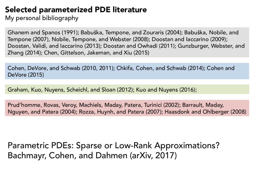
3. Selected parameterized PDE literature My personal bibliography Ghanem and Spanos (1991); Babuška, Tempone, and Zouraris (2004); Babuška, Nobile, and Tempone (2007), Nobile, Tempone, and Webster (2008); Doostan and Iaccarino (2009); Doostan, Validi, and Iaccarino (2013); Doostan and Owhadi (2011); Gunzburger, Webster, and Zhang (2014); Chen, Gittelson, Jakeman, and Xiu (2015) Cohen, DeVore, and Schwab (2010, 2011); Chkifa, Cohen, and Schwab (2014); Cohen and DeVore (2015) Prud’homme, Rovas, Veroy, Machiels, Maday, Patera, Turinici (2002); Barrault, Maday, Nguyen, and Patera (2004); Rozza, Huynh, and Patera (2007); Haasdonk and Ohlberger (2008) Graham, Kuo, Nuyens, Scheichl, and Sloan (2012); Kuo and Nuyens (2016); Parametric PDEs: Sparse or Low-Rank Approximations? Bachmayr, Cohen, and Dahmen (arXiv, 2017)
4. How many dimensions is high dimensions? Goal is to estimate … •  the solution map •  spatially varying statistics •  statistics of output of interest with as few function evaluations as possible.
5. r · (aru) = 1
6. D 1 2 The PDE The coefficients r · (aru) = 1, s 2 D u = 0, s 2 1 n · aru = 0, s 2 2 log(a(s, x)) = m X k=1 p ✓k k(s) xk Cov( s1, s2) = 2 exp ✓ ks1 s2 k1 2 ` ◆ The quantity of interest f( x ) = Z u( s , x ) d 2 •  100-term KL •  Gaussian r.v.’s Rough fields Spatial average over Neumann boundary Constantine, Dow, and Wang (2014)
7. Constantine, Dow, and Wang (2014)
8. Long length scale, ` = 1 log( a (s , x)) u( s , x ) Constantine, Dow, and Wang (2014)
9. Short length scale, log( a (s , x)) u( s , x ) ` = 0.01 Constantine, Dow, and Wang (2014)
10. f( x ) ⇢( x ) rf( x ) PDE solution’s spatial average along the Neumann boundary Standard Gaussian density Gradient computed with adjoint equations Constantine, Dow, and Wang (2014) NOT SOLUTION APPROXIMATION. NO MODEL REDUCTION IN SOLUTION SPACE.
11. C = Z rf( x ) rf( x )T ⇢( x ) d x = W ⇤W T Define the active subspace Consider a function and its gradient vector, The average outer product of the gradient and its eigendecomposition, Partition the eigendecomposition, Rotate and separate the coordinates, ⇤ =  ⇤1 ⇤2 , W = ⇥ W 1 W 2 ⇤ , W 1 2 Rm⇥n x = W W T x = W 1W T 1 x + W 2W T 2 x = W 1y + W 2z active variables inactive variables f = f( x ), x 2 Rm, rf( x ) 2 Rm, ⇢ : Rm ! R + Constantine, Dow, and Wang (2014)
12. i = Z w T i rf( x ) 2 ⇢( x ) d x , i = 1, . . . , m LEMMA Constantine, Dow, and Wang (2014) average, squared, directional derivative along eigenvector eigenvalue i > j | f( x + h wi) f( x ) | > | f( x + h wj) f( x ) | For small , on average, h WHAT DOES IT MEAN?
14. Design a jet nozzle under uncertainty (DARPA SEQUOIA project) 10-parameter engine performance model
15. Index 1 2 3 4 5 6 Eigenvalues 10-13 10-12 10-11 10-10 10-9 10-8 10-7 10-6 Est BI Index 1 2 3 4 5 6 Eigenvalues 10-13 10-12 10-11 10-10 10-9 10-8 10-7 10-6 Index 1 2 3 4 5 6 Eigenvalues 10-13 10-12 10-11 10-10 10-9 10-8 10-7 10-6 Est BI Index 1 2 3 4 5 6 Eigenvalues 10-13 10-12 10-11 10-10 10-9 10-8 10-7 10-6 Long length scale, ` = 1 Short length scale, ` = 0.01 Eigenvalues of Z rf rfT ⇢ d x
16. Parameter index 0 50 100 Eigenvector components -1 -0.5 0 0.5 1 Parameter index 0 50 100 Eigenvector components -1 -0.5 0 0.5 1 First eigenvector of Z rf rfT ⇢ d x Long length scale, ` = 1 Short length scale, ` = 0.01
17. -4 -2 0 2 4 Quantity of interest #10-3 0 1 2 3 4 5 -4 -2 0 2 4 Quantity of interest #10-4 2.4 2.6 2.8 3 3.2 3.4 3.6 3.8 Plotting versus Long length scale, ` = 1 Short length scale, ` = 0.01 f( x ) w T x w T x w T x
18. -4 -2 0 2 4 Quantity of interest 10-10 10-5 100 105 Index 0 2 4 6 Eigenvalues 10-10 100 1010 Est BI Index 0 2 4 6 Eigenvalues 10-10 100 1010 ` = 1, 2 = 1/64 w T x
19. ` = 1, 2 = 1/16 -4 -2 0 2 4 Quantity of interest 10-10 10-5 100 105 Index 0 2 4 6 Eigenvalues 10-10 100 1010 Est BI Index 0 2 4 6 Eigenvalues 10-10 100 1010 w T x
20. -4 -2 0 2 4 Quantity of interest 10-10 10-5 100 105 Index 0 2 4 6 Eigenvalues 10-10 100 1010 Est BI Index 0 2 4 6 Eigenvalues 10-10 100 1010 ` = 1, 2 = 1/4 w T x
21. -4 -2 0 2 4 Quantity of interest 10-10 10-5 100 105 Index 0 2 4 6 Eigenvalues 10-10 100 1010 Est BI Index 0 2 4 6 Eigenvalues 10-10 100 1010 ` = 1, 2 = 1 w T x
22. -4 -2 0 2 4 Quantity of interest 10-10 10-5 100 105 Index 0 2 4 6 Eigenvalues 10-10 100 1010 Est BI Index 0 2 4 6 Eigenvalues 10-10 100 1010 ` = 1, 2 = 4 w T x
23. -4 -2 0 2 4 Quantity of interest 10-10 10-5 100 105 Index 0 2 4 6 Eigenvalues 10-10 100 1010 Est BI Index 0 2 4 6 Eigenvalues 10-10 100 1010 ` = 1, 2 = 16 w T x
24. ` = 1, 2 = 64 -4 -2 0 2 4 Quantity of interest 10-10 10-5 100 105 Index 0 2 4 6 Eigenvalues 10-10 100 1010 Est BI Index 0 2 4 6 Eigenvalues 10-10 100 1010 w T x
25. ` = 0.01, 2 = 1/64 -4 -2 0 2 4 Quantity of interest #10-3 0 0.5 1 1.5 Index 1 2 3 4 5 6 Eigenvalues 10-16 10-14 10-12 10-10 10-8 10-6 Est BI Index 1 2 3 4 5 6 Eigenvalues 10-16 10-14 10-12 10-10 10-8 10-6 w T x
26. ` = 0.01, 2 = 1/16 -4 -2 0 2 4 Quantity of interest #10-3 0 0.5 1 1.5 Index 1 2 3 4 5 6 Eigenvalues 10-16 10-14 10-12 10-10 10-8 10-6 Est BI Index 1 2 3 4 5 6 Eigenvalues 10-16 10-14 10-12 10-10 10-8 10-6 w T x
27. -4 -2 0 2 4 Quantity of interest #10-3 0 0.5 1 1.5 Index 1 2 3 4 5 6 Eigenvalues 10-16 10-14 10-12 10-10 10-8 10-6 Est BI Index 1 2 3 4 5 6 Eigenvalues 10-16 10-14 10-12 10-10 10-8 10-6 ` = 0.01, 2 = 1/4 w T x
28. -4 -2 0 2 4 Quantity of interest #10-3 0 0.5 1 1.5 Index 1 2 3 4 5 6 Eigenvalues 10-16 10-14 10-12 10-10 10-8 10-6 Est BI Index 1 2 3 4 5 6 Eigenvalues 10-16 10-14 10-12 10-10 10-8 10-6 ` = 0.01, 2 = 1 w T x
29. -4 -2 0 2 4 Quantity of interest #10-3 0 0.5 1 1.5 Index 1 2 3 4 5 6 Eigenvalues 10-16 10-14 10-12 10-10 10-8 10-6 Est BI Index 1 2 3 4 5 6 Eigenvalues 10-16 10-14 10-12 10-10 10-8 10-6 ` = 0.01, 2 = 4 w T x
30. -4 -2 0 2 4 Quantity of interest #10-3 0 0.5 1 1.5 Index 1 2 3 4 5 6 Eigenvalues 10-16 10-14 10-12 10-10 10-8 10-6 Est BI Index 1 2 3 4 5 6 Eigenvalues 10-16 10-14 10-12 10-10 10-8 10-6 ` = 0.01, 2 = 16 w T x
31. -4 -2 0 2 4 Quantity of interest #10-3 0 0.5 1 1.5 Index 1 2 3 4 5 6 Eigenvalues 10-16 10-14 10-12 10-10 10-8 10-6 Est BI Index 1 2 3 4 5 6 Eigenvalues 10-16 10-14 10-12 10-10 10-8 10-6 ` = 0.01, 2 = 64 w T x
32. <2 10-2 100 102 ^ 61 =^ 62 101 102 103 104 105 <2 10-2 100 102 ^ 61 =^ 62 100 101 102 103 104 105 Long length scale, ` = 1 Short length scale, ` = 0.01 Plotting versus CONJECTURE: decreases linearly with log( 1/ 2) log( 2 ) log( 2 ) log( 1/ 2)
33. Some numerical evidence that the low- dimensional structure in some common parameterized PDEs looks like active subspaces. TODO: Prove it! PAUL CONSTANTINE Assistant Professor University of Colorado, Boulder activesubspaces.org! @DrPaulynomial! TAKE HOMES Active Subspaces SIAM (2015)