Building Deep Neural Networks & Understanding Stochastic Gradient Descent.pdf

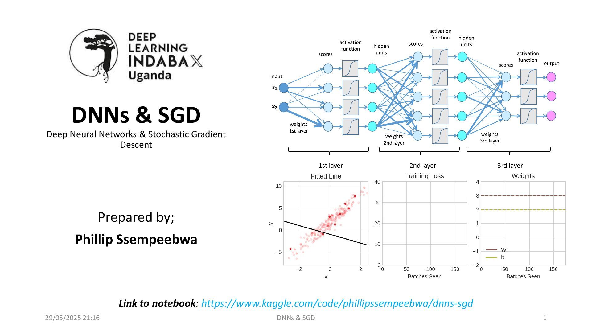
📌 Overview:
This presentation is divided into two core sections, designed to provide a foundational yet practical understanding of modern machine learning techniques: Deep Neural Networks (DNN) and Stochastic Gradient Descent (SGD). Whether you're new to neural networks or looking to strengthen your conceptual grasp, this guide bridges theory and hands-on implementation in an accessible and well-structured manner.

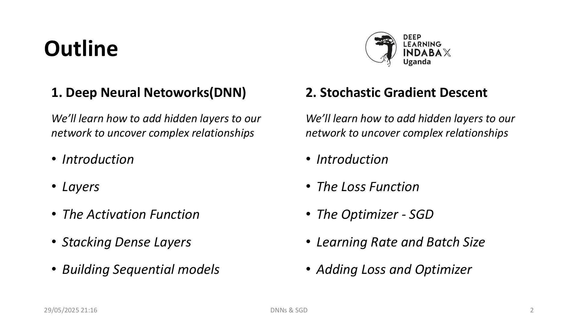
🧠 1. Deep Neural Networks (DNN)
🔍 Objective:
To understand how hidden layers in neural networks help model complex, nonlinear relationships in data.

🧱 Sections Covered:
Introduction
A brief recap of basic neural networks (input → output) and why we need more than one layer.

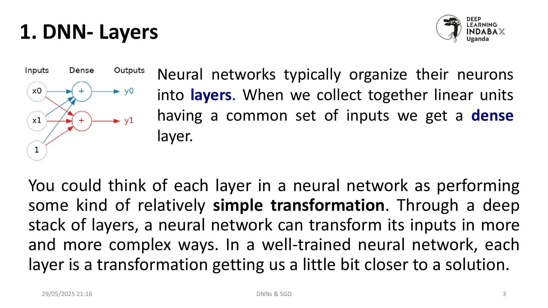
Layers
Explanation of input, hidden, and output layers, with visual representations.

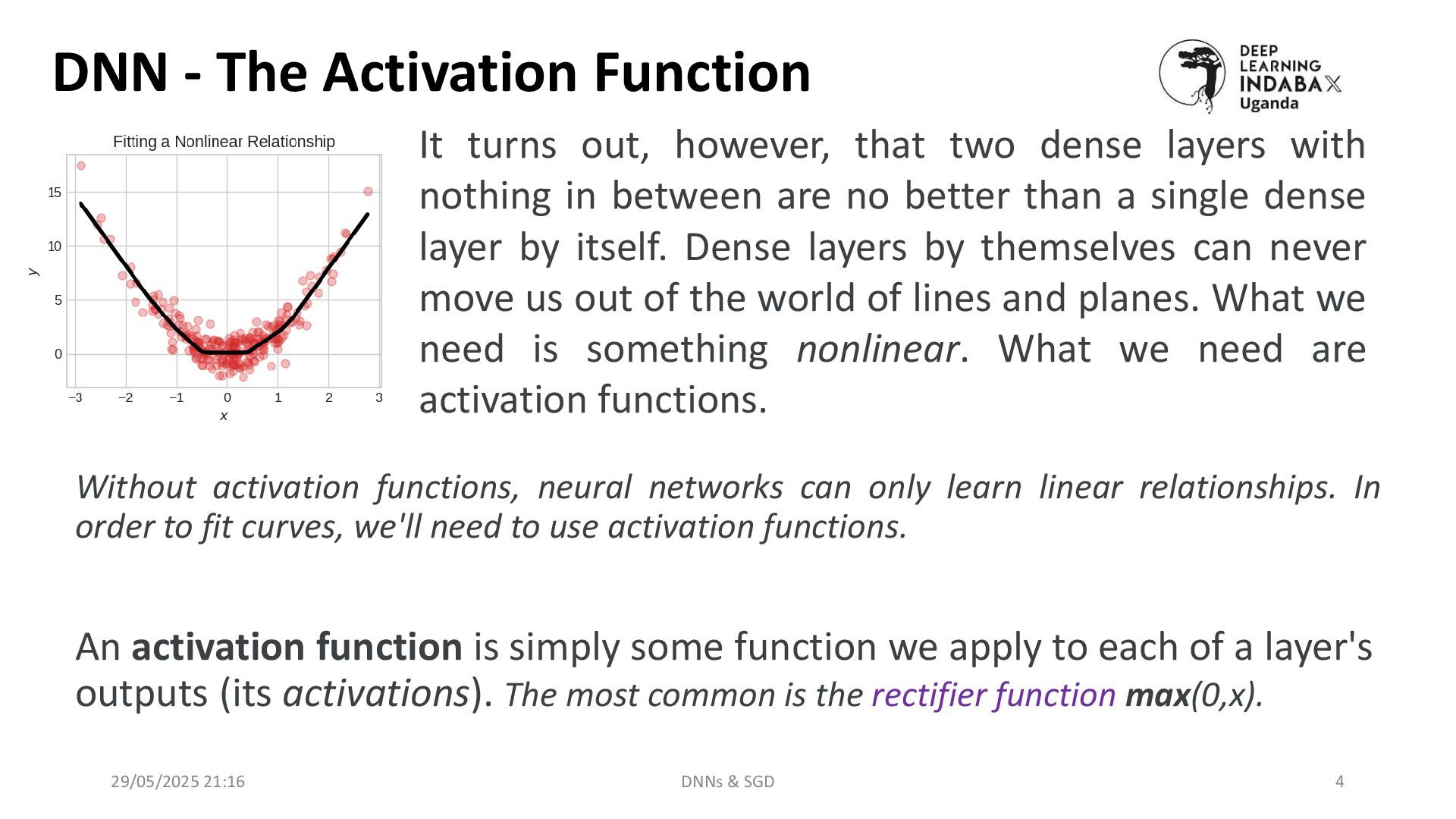
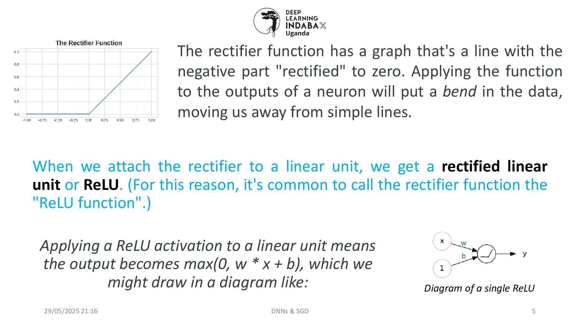
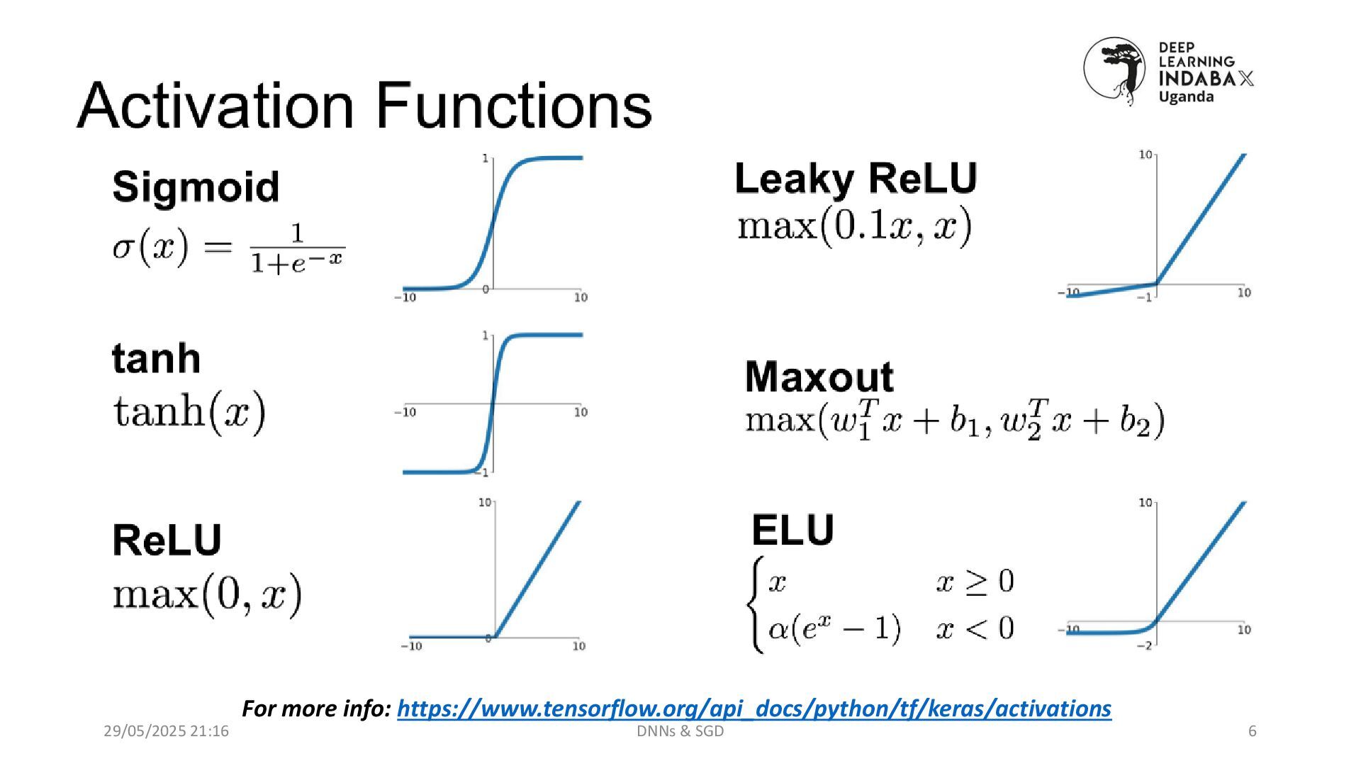
The Activation Function
Introduction to functions like ReLU, Sigmoid, and Tanh that introduce non-linearity, making neural networks powerful.

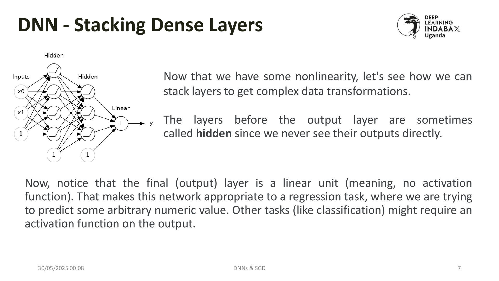
Stacking Dense Layers
How multiple layers (fully connected/dense) improve learning capacity and flexibility. Includes tips on choosing the number of layers and neurons.

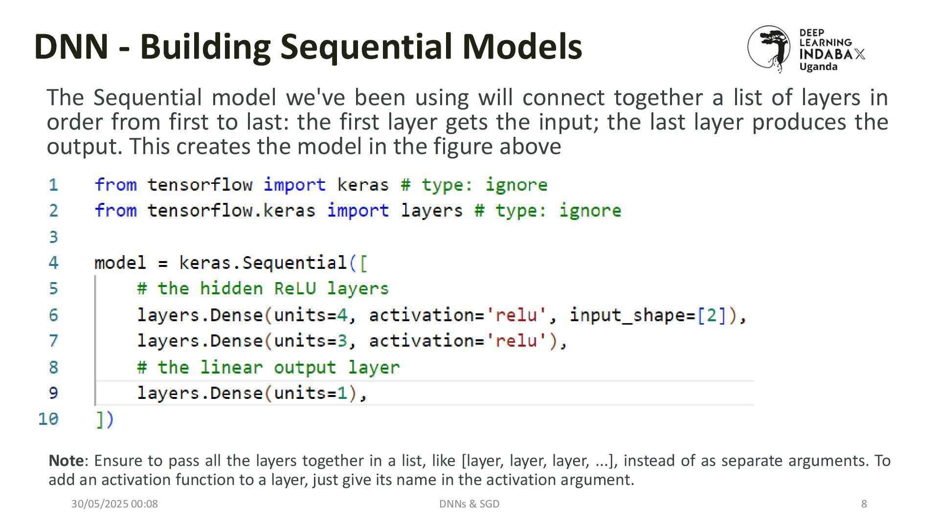
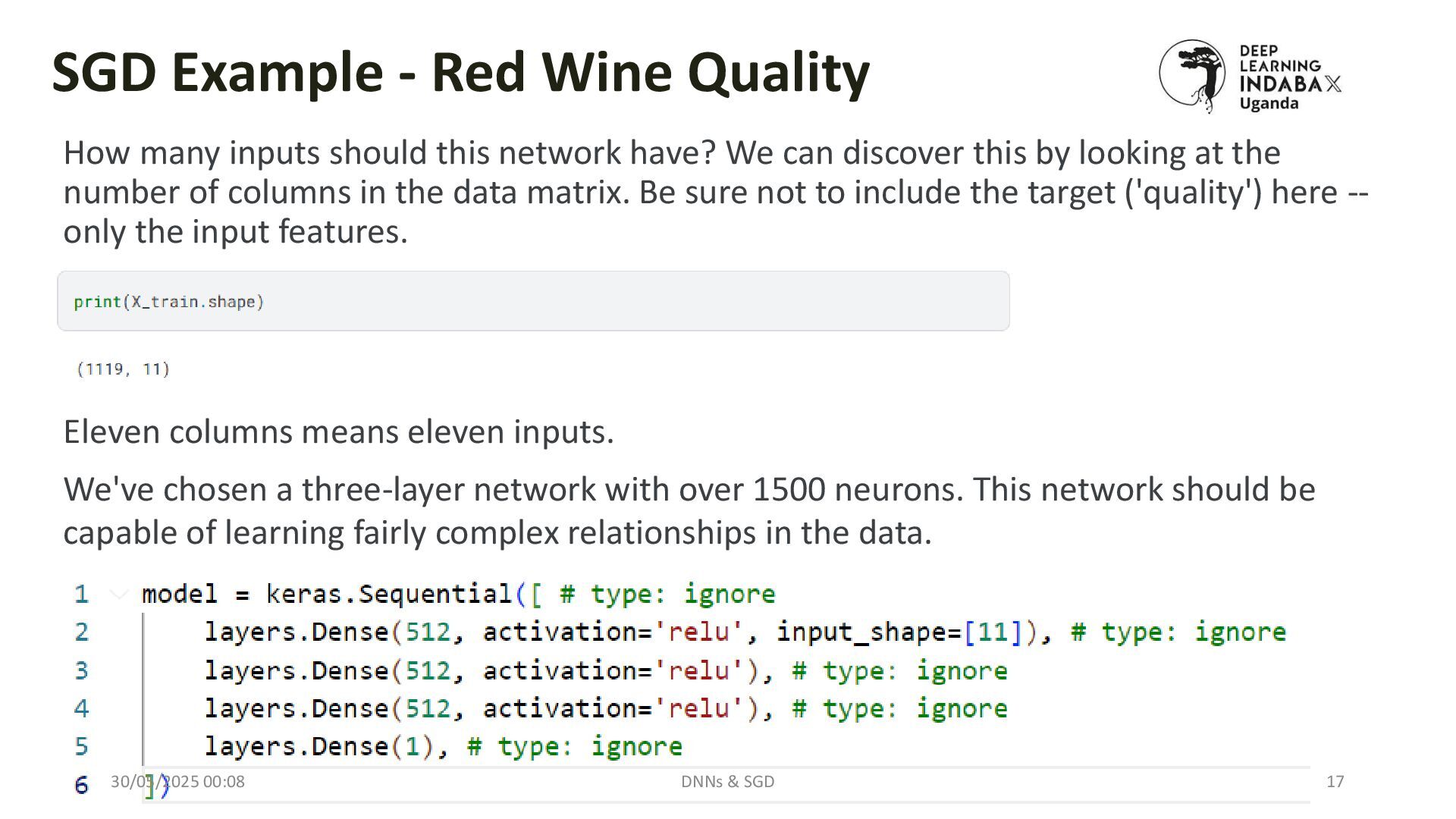
Building Sequential Models
Hands-on approach using tools like Keras/TensorFlow to build networks using the Sequential API. Covers code examples and layer-by-layer breakdowns.

⚙️ 2. Stochastic Gradient Descent (SGD)
🔍 Objective:
To understand how models are trained using loss optimization and how SGD helps reach optimal weights efficiently.

🧱 Sections Covered:
Introduction
Why we need an optimization algorithm and how it fits into the training pipeline.

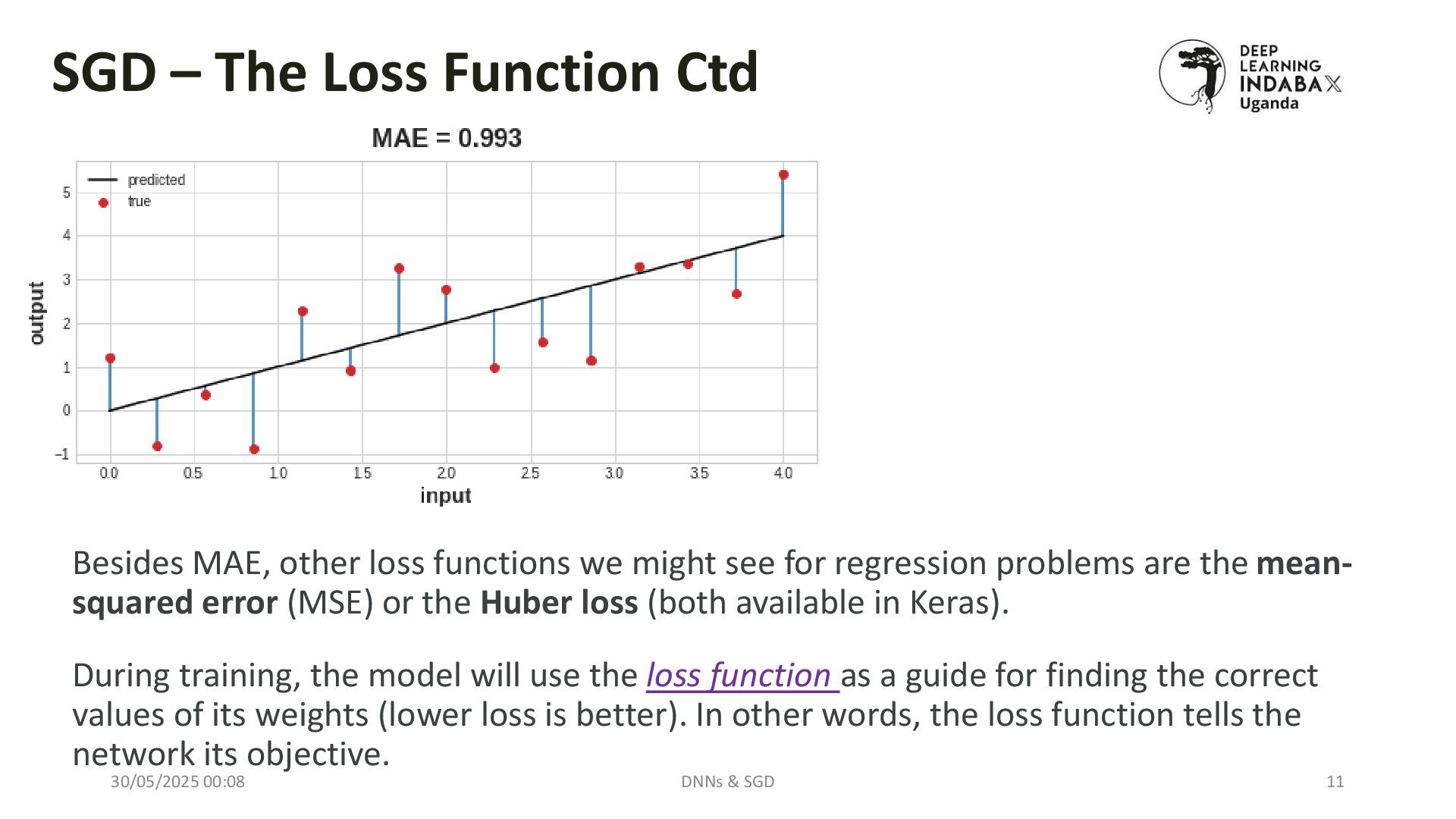
The Loss Function
Discusses how loss (e.g., MSE, CrossEntropy) measures model performance, and why minimizing it matters.

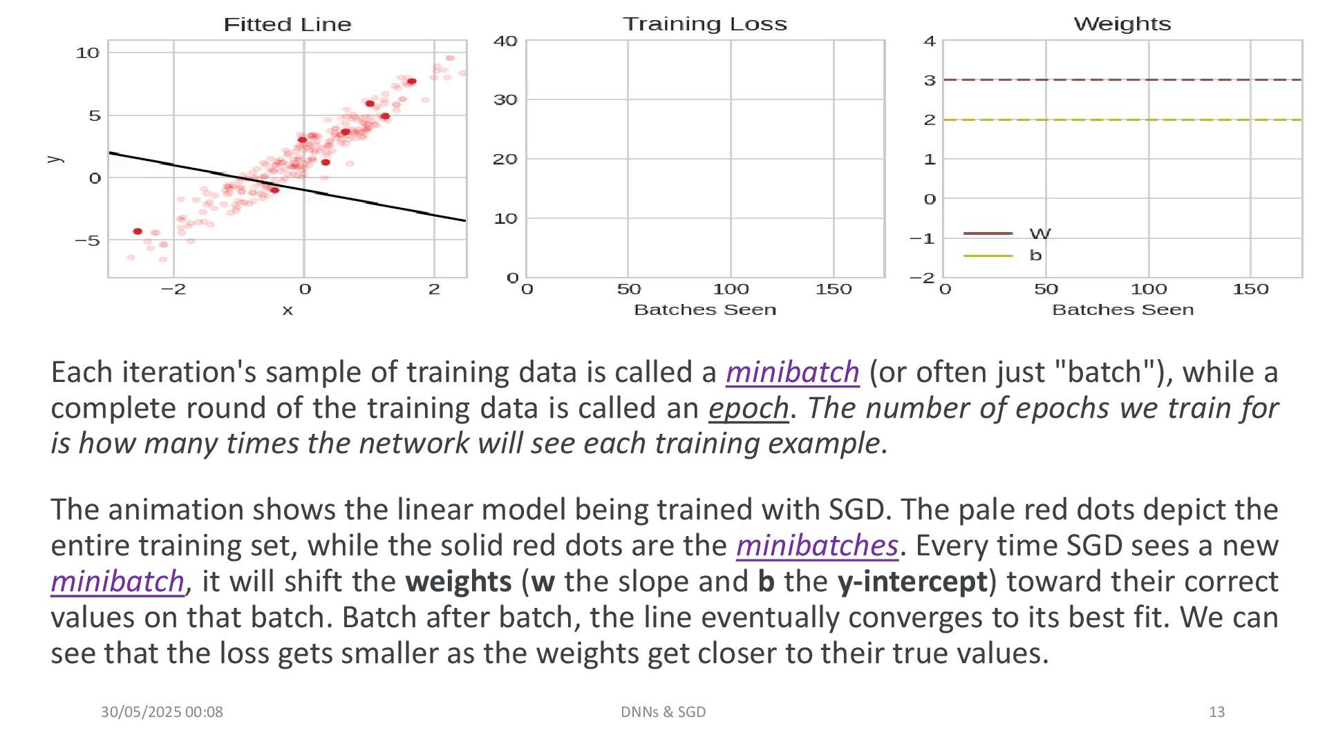
The Optimizer - SGD
In-depth explanation of Stochastic Gradient Descent, how it updates weights using small data samples, and its role in efficient learning.

Learning Rate and Batch Size
Two critical hyperparameters that influence training speed and convergence:

Learning Rate: How big the steps are toward the minimum loss

Batch Size: How many samples are used for each update

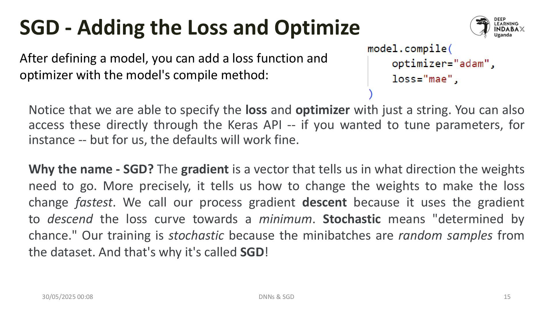
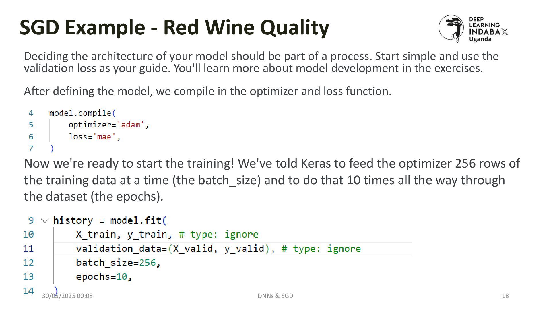
Adding Loss and Optimizer in Code
Demonstration of how to plug the loss function and SGD optimizer into a neural network using a modern ML framework.

🧰 Tools & Frameworks
Python

Keras / TensorFlow

NumPy / Matplotlib for data prep & visualization

📈 Expected Outcomes
By the end of this presentation, you will:

Understand how DNNs model complex relationships through stacked layers and nonlinear activation functions.

Know how SGD efficiently updates weights during training.

Be able to build and train a DNN using real code examples with proper loss functions and optimizers.

📎 References
https://www.tensorflow.org/learn

https://keras.io/guides/sequential_model/

https://cs231n.github.io/neural-networks-1/

https://ml-cheatsheet.readthedocs.io/en/latest/activation_functions.html

Transcript

1. DNNs & SGD Deep Neural Networks & Stochastic Gradient Descent Prepared by; Phillip Ssempeebwa Link to notebook: https://www.kaggle.com/code/phillipssempeebwa/dnns-sgd 29/05/2025 21:16 DNNs & SGD 1
2. Outline 1. Deep Neural Netoworks(DNN) We’ll learn how to add hidden layers to our network to uncover complex relationships • Introduction • Layers • The Activation Function • Stacking Dense Layers • Building Sequential models 2. Stochastic Gradient Descent We’ll learn how to add hidden layers to our network to uncover complex relationships • Introduction • The Loss Function • The Optimizer - SGD • Learning Rate and Batch Size • Adding Loss and Optimizer 29/05/2025 21:16 DNNs & SGD 2
3. 1. DNN- Layers You could think of each layer in a neural network as performing some kind of relatively simple transformation. Through a deep stack of layers, a neural network can transform its inputs in more and more complex ways. In a well-trained neural network, each layer is a transformation getting us a little bit closer to a solution. Neural networks typically organize their neurons into layers. When we collect together linear units having a common set of inputs we get a dense layer. 29/05/2025 21:16 DNNs & SGD 3
4. DNN - The Activation Function Without activation functions, neural networks can only learn linear relationships. In order to fit curves, we'll need to use activation functions. It turns out, however, that two dense layers with nothing in between are no better than a single dense layer by itself. Dense layers by themselves can never move us out of the world of lines and planes. What we need is something nonlinear. What we need are activation functions. An activation function is simply some function we apply to each of a layer's outputs (its activations). The most common is the rectifier function max(0,x). 29/05/2025 21:16 DNNs & SGD 4
5. Applying a ReLU activation to a linear unit means the output becomes max(0, w * x + b), which we might draw in a diagram like: The rectifier function has a graph that's a line with the negative part "rectified" to zero. Applying the function to the outputs of a neuron will put a bend in the data, moving us away from simple lines. When we attach the rectifier to a linear unit, we get a rectified linear unit or ReLU. (For this reason, it's common to call the rectifier function the "ReLU function".) Diagram of a single ReLU 29/05/2025 21:16 DNNs & SGD 5
6. For more info: https://www.tensorflow.org/api_docs/python/tf/keras/activations 29/05/2025 21:16 DNNs & SGD 6
7. DNN - Stacking Dense Layers The layers before the output layer are sometimes called hidden since we never see their outputs directly. Now that we have some nonlinearity, let's see how we can stack layers to get complex data transformations. Now, notice that the final (output) layer is a linear unit (meaning, no activation function). That makes this network appropriate to a regression task, where we are trying to predict some arbitrary numeric value. Other tasks (like classification) might require an activation function on the output. 30/05/2025 00:08 DNNs & SGD 7
8. DNN - Building Sequential Models The Sequential model we've been using will connect together a list of layers in order from first to last: the first layer gets the input; the last layer produces the output. This creates the model in the figure above Note: Ensure to pass all the layers together in a list, like [layer, layer, layer, ...], instead of as separate arguments. To add an activation function to a layer, just give its name in the activation argument. 30/05/2025 00:08 DNNs & SGD 8
9. SGD - Introduction Previously, we learnt how to build fully-connected networks out of stacks of dense layers. When first created, all of the network's weights are set randomly -- the network doesn't "know" anything yet. Now, we're going to see how to train a neural network; we're going to see how neural networks learn. As with all machine learning tasks, we begin with a set of training data. Each example in the training data consists of some features (the inputs) together with an expected target (the output). Training the network means adjusting its weights in such a way that it can transform the features into the target. In the 80 Cereals dataset, for instance, we want a network that can take each cereal's 'sugar', 'fiber', and 'protein' content and produce a prediction for that cereal's 'calories'. If we can successfully train a network to do that, its weights must represent in some way the relationship between those features and that target as expressed in the training data. In addition to the training data, we need two more things: A "loss function" that measures how good the network's predictions are. An "optimizer" that can tell the network how to change its weights. 30/05/2025 00:08 DNNs & SGD 9
10. SGD – The Loss Function We've seen how to design an architecture for a network, but we haven't seen how to tell a network what problem to solve. This is the job of the loss function. The loss function measures the disparity between the the target's true value and the value the model predicts. Different problems call for different loss functions. We have been looking at regression problems, where the task is to predict some numerical value -- calories in 80 Cereals, rating in Red Wine Quality. Other regression tasks might be predicting the price of a house or the fuel efficiency of a car. A common loss function for regression problems is the mean absolute error or MAE. For each prediction y_pred, MAE measures the disparity from the true target y_true by an absolute difference abs(y_true - y_pred). The total MAE loss on a dataset is the mean of all these absolute differences. 30/05/2025 00:08 DNNs & SGD 10
11. SGD – The Loss Function Ctd Besides MAE, other loss functions we might see for regression problems are the mean- squared error (MSE) or the Huber loss (both available in Keras). During training, the model will use the loss function as a guide for finding the correct values of its weights (lower loss is better). In other words, the loss function tells the network its objective. 30/05/2025 00:08 DNNs & SGD 11
12. The Optimizer - Stochastic Gradient Descent So far, we've described the problem we want the network to solve, but now we need to say how to solve it. This is the job of the optimizer. The optimizer is an algorithm that adjusts the weights to minimize the loss. Virtually all of the optimization algorithms used in deep learning belong to a family called stochastic gradient descent. They are iterative algorithms that train a network in steps. One step of training goes like this: ▪ Sample some training data and run it through the network to make predictions. ▪ Measure the loss between the predictions and the true values. ▪ Finally, adjust the weights in a direction that makes the loss smaller. Then just do this over and over until the loss is as small as you like (or until it won't decrease any further.) 30/05/2025 00:08 DNNs & SGD 12
13. Each iteration's sample of training data is called a minibatch (or often just "batch"), while a complete round of the training data is called an epoch. The number of epochs we train for is how many times the network will see each training example. The animation shows the linear model being trained with SGD. The pale red dots depict the entire training set, while the solid red dots are the minibatches. Every time SGD sees a new minibatch, it will shift the weights (w the slope and b the y-intercept) toward their correct values on that batch. Batch after batch, the line eventually converges to its best fit. We can see that the loss gets smaller as the weights get closer to their true values. 30/05/2025 00:08 DNNs & SGD 13
14. SGD - Learning Rate and Batch Size Notice that the line only makes a small shift in the direction of each batch (instead of moving all the way). The size of these shifts is determined by the learning rate. A smaller learning rate means the network needs to see more minibatches before its weights converge to their best values. The learning rate and the size of the minibatches are the two parameters that have the largest effect on how the SGD training proceeds. Their interaction is often subtle and the right choice for these parameters isn't always obvious. Fortunately, for most work it won't be necessary to do an extensive hyperparameter search to get satisfactory results. Adam is an SGD algorithm that has an adaptive learning rate that makes it suitable for most problems without any parameter tuning (it is "self tuning", in a sense). Adam is a great general-purpose optimizer. 30/05/2025 00:08 DNNs & SGD 14
15. SGD - Adding the Loss and Optimize Notice that we are able to specify the loss and optimizer with just a string. You can also access these directly through the Keras API -- if you wanted to tune parameters, for instance -- but for us, the defaults will work fine. Why the name - SGD? The gradient is a vector that tells us in what direction the weights need to go. More precisely, it tells us how to change the weights to make the loss change fastest. We call our process gradient descent because it uses the gradient to descend the loss curve towards a minimum. Stochastic means "determined by chance." Our training is stochastic because the minibatches are random samples from the dataset. And that's why it's called SGD! After defining a model, you can add a loss function and optimizer with the model's compile method: 30/05/2025 00:08 DNNs & SGD 15
16. SGD Example - Red Wine Quality Now we know everything we need to start training deep learning models. So, let's see it in action! We'll use the Red Wine Quality dataset. This dataset consists of physiochemical measurements from about 1600 Portuguese red wines. Also included is a quality rating for each wine from blind taste-tests. How well can we predict a wine's perceived quality from these measurements? We've put all of the data preparation into this next hidden cell. It's not essential to what follows so feel free to skip it. One thing you might note for now though is that we've rescaled each feature to lie in the interval [0,1][0,1]. As we'll discuss more in Lesson 5, neural networks tend to perform best when their inputs are on a common scale. 30/05/2025 00:08 DNNs & SGD 16
17. SGD Example - Red Wine Quality How many inputs should this network have? We can discover this by looking at the number of columns in the data matrix. Be sure not to include the target ('quality') here -- only the input features. Eleven columns means eleven inputs. We've chosen a three-layer network with over 1500 neurons. This network should be capable of learning fairly complex relationships in the data. 30/05/2025 00:08 DNNs & SGD 17
18. SGD Example - Red Wine Quality Deciding the architecture of your model should be part of a process. Start simple and use the validation loss as your guide. You'll learn more about model development in the exercises. After defining the model, we compile in the optimizer and loss function. Now we're ready to start the training! We've told Keras to feed the optimizer 256 rows of the training data at a time (the batch_size) and to do that 10 times all the way through the dataset (the epochs). 30/05/2025 00:08 DNNs & SGD 18
19. SGD Example - Red Wine Quality: model.fit() 30/05/2025 00:08 DNNs & SGD 19
20. You can see that Keras will keep you updated on the loss as the model trains. Often, a better way to view the loss though is to plot it. The fit method in fact keeps a record of the loss produced during training in a History object. We'll convert the data to a Pandas dataframe, which makes the plotting easy. Notice how the loss levels off as the epochs go by. When the loss curve becomes horizontal like that, it means the model has learned all it can and there would be no reason continue for additional epochs. 30/05/2025 00:08 DNNs & SGD 20
21. Thank you Link to notebook: https://www.kaggle.com/code/phillipssempeebwa/dnns-sgd 30/05/2025 00:08 DNNs & SGD 21