Using QPython in smartphones as mobile computational laboratory anywhere, anytime and anyhow by Godfrey Akpojotor

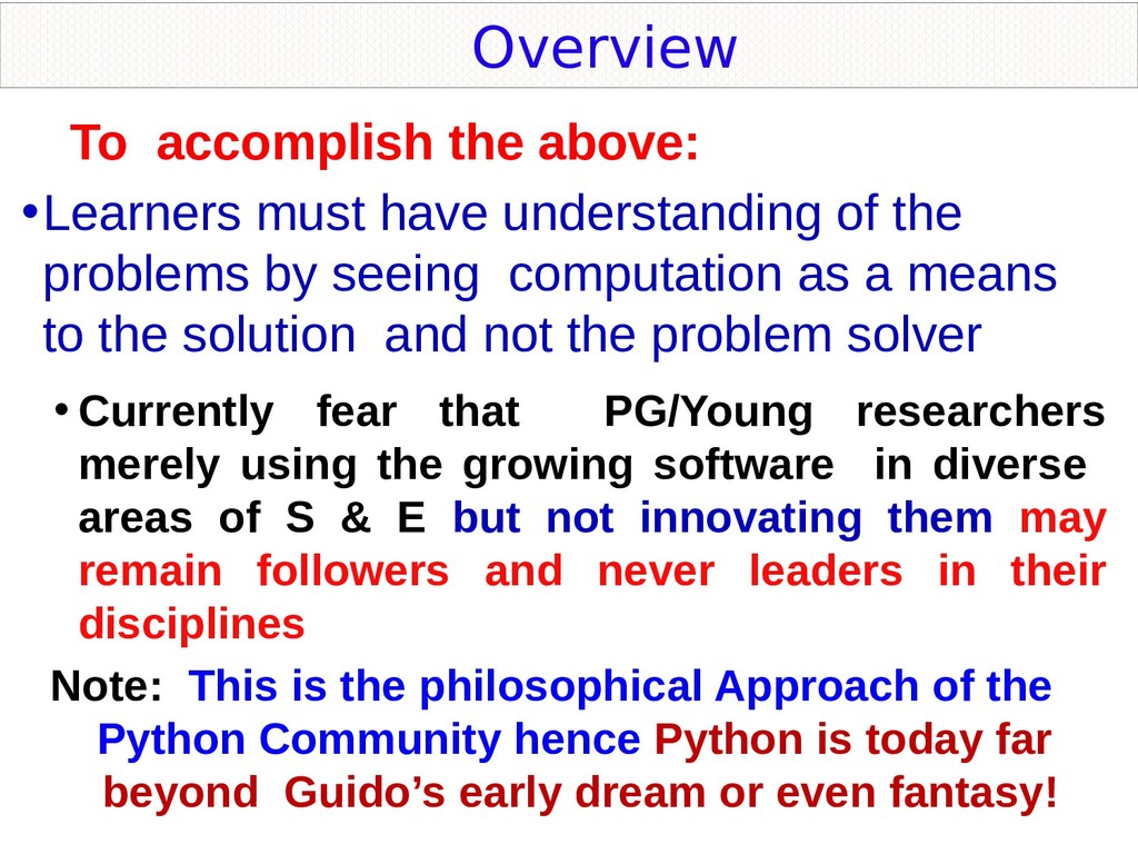
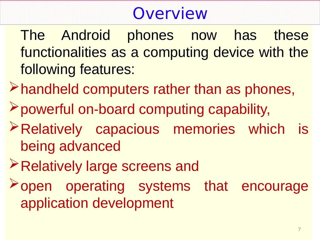
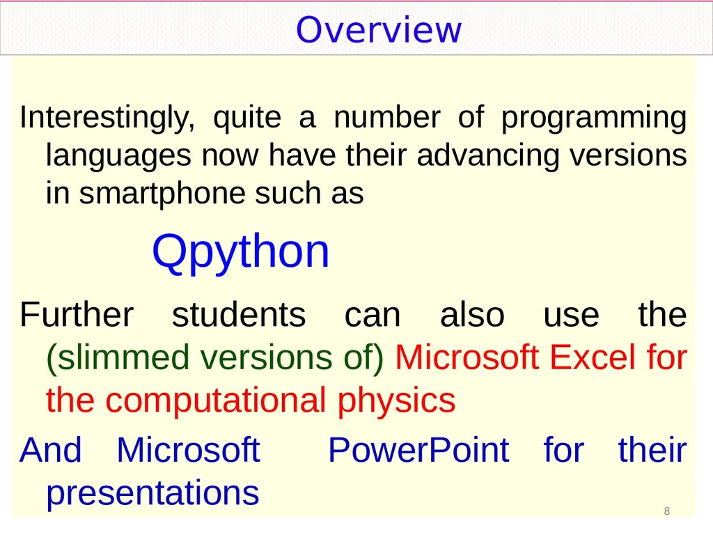
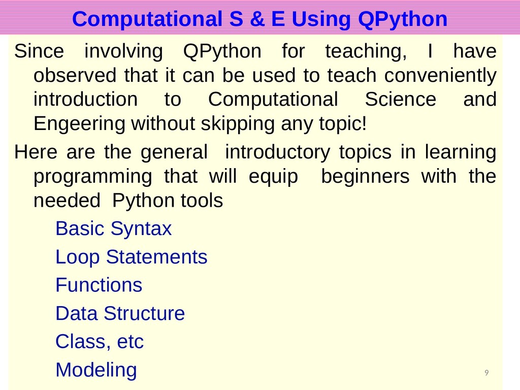
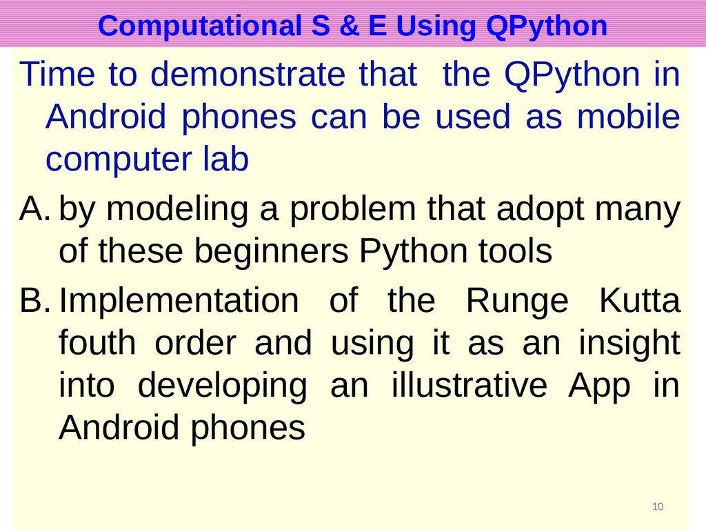
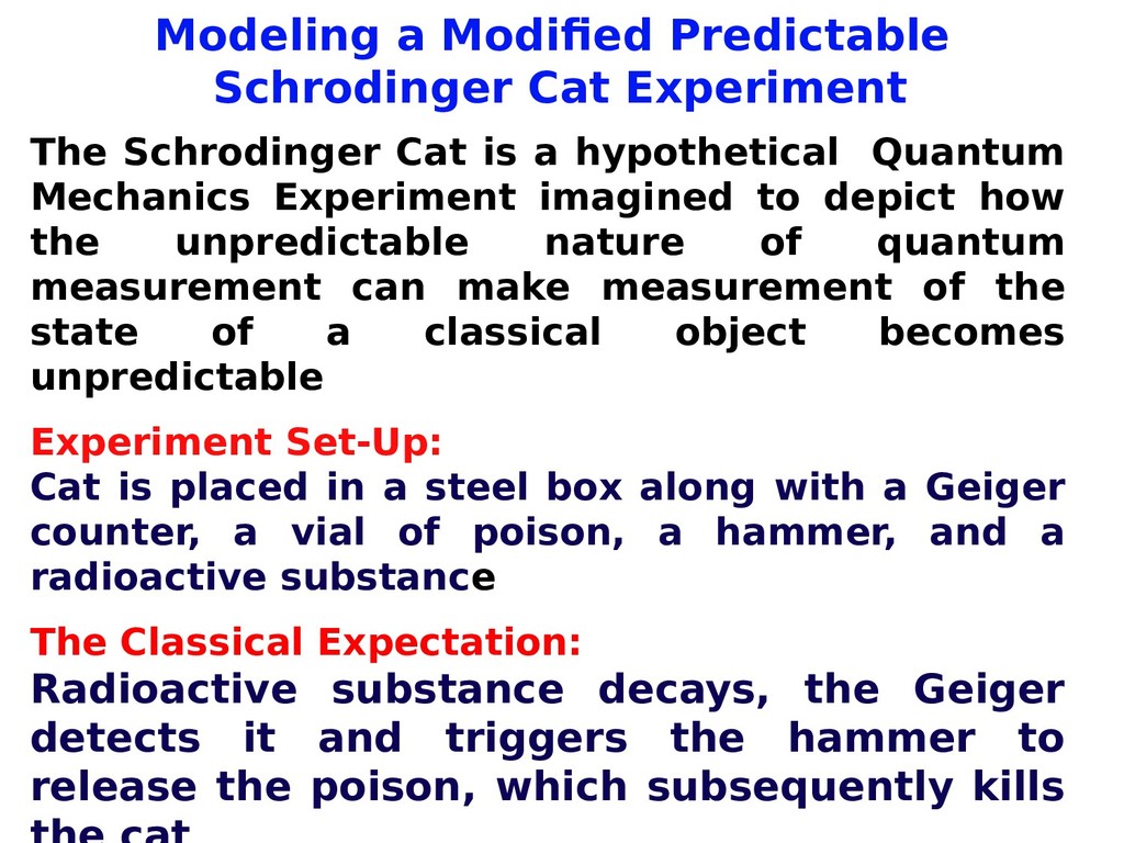
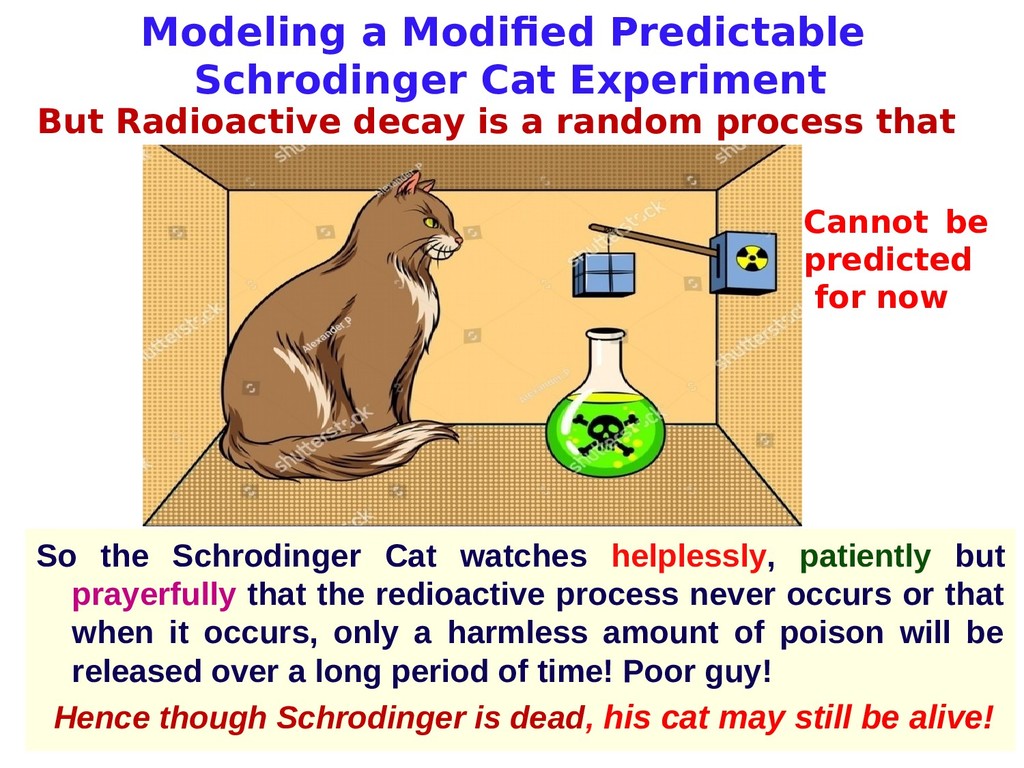
The remarkably continuous penetration of smartphones into Africa and the availability of the free and open source Python programming capabilities as QPython (QP) in smartphones meets the accessibility requirement to make them mobile computational laboratory (MCL). We present here one of our current projects under the Python African Computational Science and Engineering Tour Project (PACSETPro) of using QP as MCL for teaching programming and development of smartphone Apps to students, new beginners as well as expert programmers anywhere, anytime and anyhow.

Transcript

1. Challenges and Prospects of the Python African Computational Science and Engineering Tour Project Godfrey E. Akpojotor Physics Department, Delta State University, Abraka, Nigeria PyConZA 2014 @ Belmont Square Convention Centre, Cape Town, South Africa Thursday, October 04, 2013 Using QPython in smartphones as mobile computational laboratory anywhere, anytime and anyhow Godfrey E. Akpojotor Physics Department, Delta State University, Abraka, Nigeria Thursday, October 10, 2019 PyConZA 2019 @ The Wanderers Club, Johannesburg, South Africa 1
2. A little about me  I teach computational physics and over the years I come to realize that I am actually working in a refinery  Now when we talk about refinery, all your minds go straight to crude oil refinery where this ‘dark gold’ is refined into the various fractions such as premium motor spirit, diesel, etc.  The refinery of an academician is called the university! Delta State University, Abraka and DELSU for short  Delta State Human Refinery, Abraka and DELSHR for short while the University of Johannesburg and UJ for short Human Refinery of Johannesburg and HRJ fo short 2 Overview
3. Now in the beginning, all I wanted was to teach my computational physics course using a language that is • general-purpose to enable the students easily take skills they ;earned outside of physics • multiplatform readily available on all major operating systems • Free and easily accessible • Has many and diverse libraries so that my students are to figure out the desired library to solve diverse problems • I have pursed all these goals over the years and there are publications and my PyCon talks • All these goals motivated the PACSETPro (www.pacsetpro.com) Overview
4. • My basic philosophy: the desire to ease the learners into programming and to give them the opportunity to develop a conceptual model of what a programme is and what it does Overview
5. To accomplish the above: •Learners must have understanding of the problems by seeing computation as a means to the solution and not the problem solver • Currently fear that PG/Young researchers merely using the growing software in diverse areas of S & E but not innovating them may remain followers and never leaders in their disciplines Note: This is the philosophical Approach of the Python Community hence Python is today far beyond Guido’s early dream or even fantasy! Overview
6. * Having more and more learners access to computing devices Now the 4 functionalities of a computing device at a fundamental level: input, output, processing, and storage NEW PERPESPECTIVE Overview
7. The Android phones now has these functionalities as a computing device with the following features: handheld computers rather than as phones, powerful on-board computing capability, Relatively capacious memories which is being advanced Relatively large screens and open operating systems that encourage application development 7 NEW PERPESPECTIVE Overview
8. Interestingly, quite a number of programming languages now have their advancing versions in smartphone such as Qpython Further students can also use the (slimmed versions of) Microsoft Excel for the computational physics And Microsoft PowerPoint for their presentations 8 NEW PERPESPECTIVE OF PACSETPRO Overview
9. Since involving QPython for teaching, I have observed that it can be used to teach conveniently introduction to Computational Science and Engeering without skipping any topic! Here are the general introductory topics in learning programming that will equip beginners with the needed Python tools Basic Syntax Loop Statements Functions Data Structure Class, etc Modeling 9 Computational S & E Using QPython
10. Time to demonstrate that the QPython in Android phones can be used as mobile computer lab A. by modeling a problem that adopt many of these beginners Python tools B. Implementation of the Runge Kutta fouth order and using it as an insight into developing an illustrative App in Android phones 10 Computational S & E Using QPython
11. Modeling a Modified Predictable Schrodinger Cat Experiment The Schrodinger Cat is a hypothetical Quantum Mechanics Experiment imagined to depict how the unpredictable nature of quantum measurement can make measurement of the state of a classical object becomes unpredictable Experiment Set-Up: Cat is placed in a steel box along with a Geiger counter, a vial of poison, a hammer, and a radioactive substance The Classical Expectation: Radioactive substance decays, the Geiger detects it and triggers the hammer to release the poison, which subsequently kills
12. So the Schrodinger Cat watches helplessly, patiently but prayerfully that the redioactive process never occurs or that when it occurs, only a harmless amount of poison will be released over a long period of time! Poor guy! Hence though Schrodinger is dead, his cat may still be alive! Modeling a Modified Predictable Schrodinger Cat Experiment But Radioactive decay is a random process that Cannot be predicted for now
13. Basic Steps of Modeling Modeling is the use of programming language or mathematics applications to create an abstract model of an object, organization or processes (Akpojotor et. al., 2010) •Problem Conceptualization •Problem Formulation •Numerical Implementation •Program Design and Coding •Computation •Validation 13 Modeling a Modified Predictable Schrodinger Cat Experiment
14. Decay of Radioactive substance Detection of Radioactive particle Hammering of vile of poison Hammering of vile of poison Dying Cat Not Predictable Predictable Problem conceptualization is the step whererin a problem is transformed into a physical system Modeling a Modified Predictable Schrodinger Cat Experiment
15. 15 Choose Boundary Conditions Alive state Dead state As the amount of dose is increased from zero, the alive state of the cat will begin to decrease with increase in time but Depending on the mass of the cat . Thus the three parameters to determine the cat actual state are: * Amount of the dose of poison vile, * Time duration of exposure and * Mass of the cat Modeling a Modified Predictable Schrodinger Cat Experiment
16. 16 Heart is a muscular pump that with each heart beat pumps blood around the body. Central to this process is the heart rate because there is function of the heart called cardiac output which is directly related to heart rate and stroke volume which is the amount of blood pumped out with each beat So the heart rate is controlled by Amount of blood flowing through the heart . Modeling a Modified Predictable Schrodinger Cat Experiment
17. 17 General consensus: Cat’s health can be predicted through its heart rate which is the number of times the heart beats in the space of a minute Implication Effect of varying the amount of poison vile with time can be predicted using the heart rate of the cat depending on its mass. . Modeling a Modified Predictable Schrodinger Cat Experiment
18. 18 Interestingly: The heart rate can directly be measured by the heart pulse which in turn can be measured by the fingers to be a vibration that can be conceived simply as a to and fro movement Therefore, movement of the heart of the cat can be considered as a simple harmonic motion (SHO) Thus cat heart will be conceptualized as a SHO Generally: SHO is of great importance in physics because many more complicated systems can be treated to a good approximation as harmonic oscillator Modeling a Modified Predictable Schrodinger Cat Experiment
19. 19 Data: Though cats have many species, Cats have between 140 and 220 beats per minute (bpm) And mass range between 40 – 50 kg . Modeling a Modified Predictable Schrodinger Cat Experiment
20. 20 L n L m y y = 0 Conceptualization of the cat’s heart pulse as a SHO depicted as a mass-spring system Depicting Cat Heart as a mass-spring system
21. 21 *net force acting on the motion which can be considered as the heart beat *damping force from frictional resistance of the bob to a snapshot equivalent: resistance to the bloodflow due to the effect of the poison on heartbeat. Net force causing the simple harmonic motion is determined by Depicting Cat Heart as a mass-spring system
22. 22 The net force acting on the bob motion will be ) ( y L k mg m   where m is the mass of the bob and therefore be considered as the equivalent: mass of the cat by assuming that cat mass  heart mass k is the restoring constant and therefore be considered as the equivalent: All Effects to restore normal blood flow Depicting Cat Heart as a mass-spring system (x)
23. 23 0 2    ky bDy y mD Eq.(XX) can be re-expressed (with D = d/dt) as: which is a homogenous second order differential equation of the heart pulse with constant coefficients: m = mass of cat  heart mass b = damping constant considered as the amount of poison k = pumping of the blood in the heart Combining the two forces responsible for the oscillatory motion of the bob leads to dt dy b ky dt y d m    2 2 (1) Depicting Cat Heart as a mass-spring system (xx)
24. 24 Eq.(1) can then be resolved using the auxiliary equation method to obtain the possible roots as km b m m b D 4 2 1 2 2 1     km b m m b D 4 2 1 2 2 2     Resulting in 3 cases hence 3 different oscillatory motions as we vary the m, b and k: 0 4 2   km b 0 4 2   km b 0 4 2   km b Under dosing Critical dosing Over dosing. (2a) (2b) (3b) (3a) (3c) Depicting Cat Heart as a mass-spring system
25. Underdosing: Cat normal state when amount of poison is zero or very small so that cat heart beat is normal Critical dosing: Cat abnormal state when amount of poison is now large to cause maximum abnormal heart beat Overdosing: Cat death state when amount of poison is too large for the heart to beat 25 Depicting Cat Heart as a mass-spring system
26. Program Design and Coding in QPython • Sort I • Eq.(1) is a Quadratic function hence a polynomial of degree 2 • In Python: can easily use the poly1d function in NumPy but Numpy is not readily stable in Qpython now • So in QPython: use the lambda expression in Math Module to create anonymous functions, • Note: Lambda functions originate from Lambda Calculus and therefore are different from normal Python functions, though we can always replace a lambda function by a Python Function 26
27. Program Design and Coding in QPython • Sort II • sqrt function is in Math Module • But the under dose case (Eq. (3a)): of Eq. (1) will result a complex root. • In Python can use scipy directly or from numpy.lib.scimath import sqrt • In QPython: Use cmath - complex math module which however converts all date type to complex hence: from cmath import* 27 0 4 2   km b
28. Program Design and Coding in QPython 28 Because of good knowledge of Quadratic equation And Simple harmonic oscillator One solution is for time And the second for Energy
29. 29 from math import* import cmath def MsceQuadratic(m,k): for b in range(46, 50, 1): y = lambda x: m*t**2 + b*t + k print ('At m = %g kg, b = %g m/l, k = %g pm'%(m,b,k)) if (b**2 - 4*m*k) < 0: t1 = (-b-cmath.sqrt(b**2-4*m*k))/(2.0*k) T = abs(t1.real) t2 = (-b+cmath.sqrt(b**2-4*m*k))/(2.0*k) E = abs(t2.imag) print ('T = %7f s' %(T)) print ('E = %7f s' %(E)) #print (t2) print ('This is underdosing') elif (b**2 - 4*m*k) == 0: T = (-b-sqrt(b**2-4*m*k))/(2.0*k) E = (-b+sqrt(b**2-4*m*k))/(2.0*k) print ('T = %7f' %(T)) print ('E = %7f' %(E)) print ('critical dosing') elif (b**2 - 4*m*k) > 0: T = abs((-b-sqrt(b**2-4*m*k))/(2.0*k)) E = (-b+sqrt(b**2-4*m*k))/(2.0*k) print ('T = %7f s' %(T)) print ('E = %7f' %(E)) #print (abs(t2)) print ('overdosing')
30. Program Design and Coding • Simple Run 30 >>> MsceQuadratic(4, 140) At m = 4 kg, b = 46 m/l, k = 140 bpm T = 0.164286 s E = 0.039770 s This is underdosing At m = 4 kg, b = 47 m/l, k = 140 bpm T = 0.167857 s E = 0.019885 s This is underdosing At m = 4 kg, b = 48 m/l, k = 140 bpm T = 0.200000 s E = -0.142857 overdosing At m = 4 kg, b = 49 m/l, k = 140 bpm T = 0.220316 s E = -0.129684 overdosing
31. Program Design and Coding 31 Observe that the critical dosing requires us to have float point interval This is where ‘while’ has an edge in math module over ‘for’
32. from math import* import cmath def MsceQuadratic(m,b,k, db): while b <= 48: y = lambda x: m*t**2 + b*t + k - - - - - - - - -- - - - - - -- - - - - - - - - - >>> MsceQuadratic(4, 47, 140,0.5) At m = 4 kg, b = 47 m/l, k = 140 bpm T = 0.167857 s E = 0.0198849 s This is underdosing At m = 4 kg, b = 47.3286 m/l, k = 140 bpm T = 0.169031 s E = -0.169031 s critical dosing At m = 4 kg, b = 47.5 m/l, k = 140 bpm T = 0.184040 s E = -0.155246 s overdosing
33. General trend of the numerical results: As the cat is exposed to the poison with increasing time, Cat goes from normal alive state to critical alive state to dead state With the energy decreasing from normal state to dead state And amount of poison for the 3 states increasing with cat masses which are as expected Numerical Results
34. Quick Glance of Runge Kutta Equation • Obviously, the under dose case (Eq. (XXX)): • in Eq. (XXX) will result a complex root. • In Python, we ca use use the scipy directly or from numpy.lib.scimath import sqrt • Fortunately there is complex module in Qpython: cmath which however converts all date type to complex. • So we cannot use the command • from cmath import* • Instead we have import both the math and cmath modules • from math import* or • import math • Import cmath 34 0 4 2   km b Purpose of study here: Implementation of the Runge Kutta fourth order Equation for first order differential equation (using Radioactive decay equation as an example) and to give an insight into an illustrative App in Android phones
35. Quick Glance of Runge Kunta Equation There are many version of the Runge Kutta equation But all the version and approach here can be applied to them For an initial value problem given by 0 0 ) ( , ) , ( y x y y x f y    where y is an unknown function (scalar or vector) of x, and therefore whose approximate solution we seek. Starting from the initial conditions and 0 x 0 y
36. Quick Glance of Runge Kutta Equation 36 Runge-Kutta fourth order equation: where ) 2 2 ( 6 1 4 3 2 1 1 k k k k y y n n         3 4 2 3 1 2 1 , 2 , 2 2 , 2 ) , ( k y h x hf k k y h x hf k k y h x hf k y x hf k n n n n n n n n                      
37. 37 QPython Impementation of Runge Kutta Equation Radioactive decay First order ODE: Radioactive decay equation N dt dN    time life half sample of quantity 2 ln : where     t T N T 
38. 38 QPython Impementation of Runge Kutta Equation Radioactive decay To implement the Radioactive decay equation We need to modify the equation for that particular problem For: The decay of 0.05g Isotope half life of 2.40 years after half a year and 1 year Input x = 0 y = 0.05. Minimum Range = 0 Maximum Range = 1 (1 year) h = 0.5
39. 39 QPython Impementation of Runge Kutta Equation print("enter x") x = float(input()); print("enter y") y = float(input()); print("enter minrange") minRange = float(input()); print("enter maxrange") maxRange = float(input()); print("enter h") h = float(input()); k1 = 0; k2 = 0; k3 = 0; k4 = 0; print ('x y') #this is the function that holds the question’s formula def f(x,y): #return (‘function to be resolved’) return (-((math.log(2))/5.27)*y)
40. 40 QPython Impementation of Runge Kutta Equation def frange(start, stop, jump): while start < (stop): yield start start += jump for i in frange(minRange, maxRange, h): k1 = h * f(x, y); k2 = h * f(x+(h/2), y+(k1/2)); k3 = h * f(x+(h/2), y+(k2/2)); k4 = h * f(x+h, y+k3); #update the value of x and y x = x + h; #this line increases x to maxrange y = y +(1/6)*(k1 + (2*k2) + (2*k3) + k4); #print out each x, y value in the loop; print("%4.1f %5.5f" % (x, y))
41. 41 QPython Impementation of Runge Kutta Equation def frange(start, stop, jump): while start < (stop): yield start start += jump for i in frange(minRange, maxRange, h): k1 = h * f(x, y); k2 = h * f(x+(h/2), y+(k1/2)); k3 = h * f(x+(h/2), y+(k2/2)); k4 = h * f(x+h, y+k3); #update the value of x and y x = x + h; #this line increases x to maxrange y = y +(1/6)*(k1 + (2*k2) + (2*k3) + k4); #print out each x, y value in the loop; print("%4.1f %5.5f" % (x, y))
42. 42 Numerical Results Element Mass number Half life(yr) Initial mass(g) (0.5)year 1 year Tritium 3 12.26 0.05 0.04861 0.04725 Neon 22 260 0.05 0.04993 0.04987 Silicon 32 700 0.05 0.04998 0.04995 Argon 39 270 0.05 0.04994 0.04987 Argon 42 33 0.05 0.04948 0.04896 Titanium 44 47 0.05 0.04963 0.04927 Iron 55 2.4 0.05 0.04328 0.03746 Cesium 134 2.1 0.05 0.04239 0.03594
43. Insight into Illustrative App • Using the entries is already laying a coding foundation to build an illustrative App which is an (Akpojotor, 2016) • Students are always interested in how to develop Androids Apps using Python and QPython • Problem why I have not extended my study in that direction is that the Physics curriculum is already choke up • But I do lay the foundation using Kivy • 43
44. Thank you 44