Upgrade to Pro — share decks privately, control downloads, hide ads and more …

Statistical Rethinking 2022 Lecture 03

Statistical Rethinking 2022 Lecture 03

Richard McElreath

January 10, 2022
Tweet

More Decks by Richard McElreath

Other Decks in Education

Transcript

  1. Geocentrism • Descriptively accurate • Mechanistically wrong • General method

    of approximation • Known to be wrong Linear Regression • Descriptively accurate • Mechanistically wrong • General method of approximation • Taken too seriously
  2. Simple statistical golems Model of mean and variance of variable

    Mean as weighted sum of other variables Many special cases: ANOVA, ANCOVA, t-test, MANOVA Can also be generative models Linear Regression From Breath of Bones: A Tale of the Golem
  3. Why Normal? Two arguments (1) Generative: Summed fluctuations tend towards

    normal distribution (2) Statistical: For estimating mean and variance, normal distribution is least informative distribution (maxent) Variable does not have to be normally distributed for normal model to be useful
  4. Making Normal Models Goals: (1) Language for representing models (2)

    How to calculate bigger posterior distributions (3) Constructing & understanding linear models
  5. Language for modeling Revisit globe tossing model: outcome “is distributed”

    W ~ Binomial(N, p) p ~ Uniform(0, 1) data distribution (likelihood)
  6. Language for modeling Revisit globe tossing model: outcome parameter
 to

    estimate “is distributed” W ~ Binomial(N, p) p ~ Uniform(0, 1) data distribution (likelihood)
  7. Language for modeling Revisit globe tossing model: outcome parameter
 to

    estimate prior distribution “is distributed” W ~ Binomial(N, p) p ~ Uniform(0, 1) data distribution (likelihood)
  8. Now make it compute — arrange as probability statements W

    p Pr(W|N, p) = Pr(p) = Binomial( Uniform( N, p) 0, 1) | |
  9. Now make it compute — arrange as probability statements W

    p Pr(W|N, p) = Pr(p) = Binomial( Uniform( N, p) 0, 1) | | Pr(p|W, N) ∝ Binomial(W|N, p) Uniform(p|0,1) “proportional to” Posterior distribution
  10. Now make it compute — using code Pr(p|W, N) ∝

    Binomial(W|N, p) Uniform(p|0,1) W <- 6 N <- 9 p <- seq(from=0,to=1,len=1000) PrW <- dbinom(W,N,p) Prp <- dunif(p,0,1) posterior <- PrW * Prp
  11. Linear Regression Drawing the Owl (1) Question/goal/estimand (2) Scientific model

    (3) Statistical model(s) (4) Validate model (5) Analyze data
  12. Linear Regression Drawing the Owl (1) Question/goal/estimand (2) Scientific model

    (3) Statistical model(s) (4) Validate model (5) Analyze data library(rethinking) data(Howell1) 60 80 100 140 180 10 20 30 40 50 60 height (cm) weight (kg)
  13. Linear Regression Drawing the Owl (1) Question/goal/estimand Describe association between

    weight and height library(rethinking) data(Howell1) 60 80 100 140 180 10 20 30 40 50 60 height (cm) weight (kg)
  14. Linear Regression Drawing the Owl (1) Question/goal/estimand Describe association between

    ADULT weight and height data(Howell1) d <- Howell1[Howell1$age>=18,] 140 150 160 170 180 30 35 40 45 50 55 60 height (cm) weight (kg)
  15. Linear Regression (2) Scientific model How does height influence weight?

    140 150 160 170 180 30 35 40 45 50 55 60 height (cm) weight (kg) data(Howell1) d <- Howell1[Howell1$age>=18,] H W W = f(H) “Weight is some function of height”
  16. Generative models Options (1) Dynamic: Incremental growth of organism; both

    mass and height (length) derive from growth pattern; Gaussian variation result of summed fluctuations
  17. Generative models Options (1) Dynamic: Incremental growth of organism; both

    mass and height (length) derive from growth pattern; Gaussian variation result of summed fluctuations (2) Static: Changes in height result in changes in weight, but no mechanism; Gaussian variation result of growth history
  18. y i = α + βx i index intercept slope

    Anatomy of a linear model
  19. μ i = α + βx i y i ∼

    Normal(μ i , σ) expectation standard
 deviation Anatomy of a linear model “Each x value has a different expectation, E(y|x) = µ”
  20. Generative model: H → W μ i = α +

    βH i W i ∼ Normal(μ i , σ) alpha <- 0 beta <- 0.5 sigma <- 5 n_individuals <- 100 H <- runif(n_individuals,130,170) mu <- alpha + beta*H W <- rnorm(n_individuals,mu,sigma)
  21. Generative model: H → W μ i = α +

    βH i W i ∼ Normal(μ i , σ) alpha <- 0 beta <- 0.5 sigma <- 5 n_individuals <- 100 H <- runif(n_individuals,130,170) mu <- alpha + beta*H W <- rnorm(n_individuals,mu,sigma)
  22. Generative model: H → W μ i = α +

    βH i W i ∼ Normal(μ i , σ) alpha <- 0 beta <- 0.5 sigma <- 5 n_individuals <- 100 H <- runif(n_individuals,130,170) mu <- alpha + beta*H W <- rnorm(n_individuals,mu,sigma)
  23. Generative model: H → W μ i = α +

    βH i W i ∼ Normal(μ i , σ) alpha <- 0 beta <- 0.5 sigma <- 5 n_individuals <- 100 H <- runif(n_individuals,130,170) mu <- alpha + beta*H W <- rnorm(n_individuals,mu,sigma)
  24. Generative model: H → W μ i = α +

    βH i W i ∼ Normal(μ i , σ) alpha <- 0 beta <- 0.5 sigma <- 5 n_individuals <- 100 H <- runif(n_individuals,130,170) mu <- alpha + beta*H W <- rnorm(n_individuals,mu,sigma) 130 140 150 160 170 55 60 65 70 75 80 85 90 height (cm) weight (kg) Synthetic people!
  25. Linear Regression Drawing the Owl (1) Question/goal/estimand (2) Scientific model

    (3) Statistical model(s) (4) Validate model (5) Analyze data 140 150 160 170 180 30 35 40 45 50 55 60 height (cm) weight (kg) data(Howell1) d <- Howell1[Howell1$age>=18,]
  26. μ i = α + βx i y i ∼

    Normal(μ i , σ) Anatomy of a linear model α ∼ Normal(0,1) β ∼ Normal(0,1) σ ∼ Uniform(0,1)
  27. Sampling the prior distribution n_samples <- 10 alpha <- rnorm(n_samples,0,1)

    beta <- rnorm(n_samples,0,1) plot(NULL,xlim=c(-2,2),ylim=c(-2,2), xlab="x",ylab="y") for ( i in 1:n_samples ) abline(alpha[i],beta[i],lwd=4,col=2) -2 -1 0 1 2 -2 -1 0 1 2 x y
  28. Statistical model for H → W Structure of statistical model

    similar to generative model, BUT (1) Useful to re-scale variables (2) Must think about priors These two things go together μ i = α + β(H i − ¯ H) W i ∼ Normal(μ i , σ) α ∼ Normal(?, ?) β ∼ Normal(?, ?) σ ∼ Uniform(0,?)
  29. Statistical model for H → W Re-scaling height so that

    the intercept makes sense μ i = α + β(H i − ¯ H) W i ∼ Normal(μ i , σ) H i − ¯ H α value of µ when H i − ¯ H = 0 mean value of H i
  30. Statistical model for H → W Now what are scientifically

    reasonable priors? : average adult weight : kilograms per centimeter μ i = α + β(H i − ¯ H) W i ∼ Normal(μ i , σ) α ∼ Normal(60,10) β ∼ Normal(0,10) σ ∼ Uniform(0,10)
  31. Sampled regression lines n <- 10 alpha <- rnorm(n,60,10) beta

    <- rnorm(n,0,10) Hbar <- 150 Hseq <- seq(from=130,to=170,len=30) plot(NULL,xlim=c(130,170),ylim=c(10,100), xlab="height (cm)",ylab="weight (kg)") for ( i in 1:n ) lines( Hseq , alpha[i] + beta[i]*(Hseq-Hbar) , lwd=3 , col=2 )
  32. Sampled regression lines n <- 10 alpha <- rnorm(n,60,10) beta

    <- rnorm(n,0,10) Hbar <- 150 Hseq <- seq(from=130,to=170,len=30) plot(NULL,xlim=c(130,170),ylim=c(10,100), xlab="height (cm)",ylab="weight (kg)") for ( i in 1:n ) lines( Hseq , alpha[i] + beta[i]*(Hseq-Hbar) , lwd=3 , col=2 )
  33. Sampled regression lines n <- 10 alpha <- rnorm(n,60,10) beta

    <- rnorm(n,0,10) Hbar <- 150 Hseq <- seq(from=130,to=170,len=30) plot(NULL,xlim=c(130,170),ylim=c(10,100), xlab="height (cm)",ylab="weight (kg)") for ( i in 1:n ) lines( Hseq , alpha[i] + beta[i]*(Hseq-Hbar) , lwd=3 , col=2 ) 130 140 150 160 170 20 40 60 80 100 height (cm) weight (kg)
  34. Statistical model for H → W μ i = α

    + β(H i − ¯ H) W i ∼ Normal(μ i , σ) α ∼ Normal(60,10) β ∼ LogNormal(0,1) σ ∼ Uniform(0,10) 0 1 2 3 4 5 0.0 0.5 1.0 1.5 simulated b values Density
  35. Sampled regression lines n <- 10 alpha <- rnorm(n,60,10) beta

    <- rlnorm(n,0,1) Hbar <- 150 Hseq <- seq(from=130,to=170,len=30) plot(NULL,xlim=c(130,170),ylim=c(10,100), xlab="height (cm)",ylab="weight (kg)") for ( i in 1:n ) lines( Hseq , alpha[i] + beta[i]*(Hseq-Hbar) , lwd=3 , col=2 ) 130 140 150 160 170 20 40 60 80 100 height (cm) weight (kg)
  36. Sermon on Priors There are no correct priors, only scientifically

    justifiable priors Justify with information outside the data — like rest of model Priors not so important in simple linear models But need to practice now: simulate, understand, expand 130 140 150 160 170 20 40 60 80 100 height (cm) weight (kg)
  37. Fitting the model Posterior is Pr(α, β, σ|W, H) μ

    i = α + β(H i − ¯ H) W i ∼ Normal(μ i , σ) α ∼ Normal(60,10) β ∼ LogNormal(0,1) σ ∼ Uniform(0,10) Pr(W i |μ i , σ) Pr(α) Pr(β) Pr(σ)
  38. Fitting the model Normal(W|μ, σ) Normal(α|60,10) LogNormal(β|0,1) Uniform(σ|0,10) Pr(α, β,

    σ|W, H) ∝ × × × Grid approximation expensive:
 100 values of each parameter => 1 million calculations See page 85 in book for coded example
  39. Approximate posterior Many posterior distributions are approximately Gaussian Instead of

    grid approximation, Gaussian approximation Sometimes called quadratic or Laplace approximation See page 41 in book for more detail
  40. Linear Regression Drawing the Owl (1) Question/goal/estimand (2) Scientific model

    (3) Statistical model(s) (4) Validate model (5) Analyze data 140 150 160 170 180 30 35 40 45 50 55 60 height (cm) weight (kg) data(Howell1) d <- Howell1[Howell1$age>=18,]
  41. Simulation-Based Validation Bare minimum: Test statistical model with simulated observations

    from scientific model Golem might be broken Even working golems might not deliver what you hoped Strong test: Simulation-Based Calibration Fahrvergnügen
  42. Model formula W ~ dnorm(mu,sigma), mu <- a + b*(H-Hbar),

    a ~ dnorm(60,10), b ~ dlnorm(0,1), sigma ~ dunif(0,10) μ i = α + β(H i − ¯ H) W i ∼ Normal(μ i , σ) α ∼ Normal(60,10) β ∼ LogNormal(0,1) σ ∼ Uniform(0,10)
  43. First validate with simulation alpha <- 70 beta <- 0.5

    sigma <- 5 n_individuals <- 100 H <- runif(n_individuals,130,170) mu <- alpha + beta*(H-mean(H)) W <- rnorm(n_individuals,mu,sigma) dat <- list( H=H , W=W , Hbar=mean(H) ) m_validate <- quap( alist( W ~ dnorm(mu,sigma), mu <- a + b*(H-Hbar), a ~ dnorm(60,10), b ~ dlnorm(0,1), sigma ~ dunif(0,10) ), data=dat ) 130 140 150 160 170 55 60 65 70 75 80 85 H W
  44. First validate with simulation alpha <- 70 beta <- 0.5

    sigma <- 5 n_individuals <- 100 H <- runif(n_individuals,130,170) mu <- alpha + beta*(H-mean(H)) W <- rnorm(n_individuals,mu,sigma) dat <- list( H=H , W=W , Hbar=mean(H) ) m_validate <- quap( alist( W ~ dnorm(mu,sigma), mu <- a + b*(H-Hbar), a ~ dnorm(60,10), b ~ dlnorm(0,1), sigma ~ dunif(0,10) ), data=dat ) 130 140 150 160 170 55 60 65 70 75 80 85 H W
  45. First validate with simulation alpha <- 70 beta <- 0.5

    sigma <- 5 n_individuals <- 100 H <- runif(n_individuals,130,170) mu <- alpha + beta*(H-mean(H)) W <- rnorm(n_individuals,mu,sigma) dat <- list( H=H , W=W , Hbar=mean(H) ) m_validate <- quap( alist( W ~ dnorm(mu,sigma), mu <- a + b*(H-Hbar), a ~ dnorm(60,10), b ~ dlnorm(0,1), sigma ~ dunif(0,10) ), data=dat ) 130 140 150 160 170 55 60 65 70 75 80 85 H W
  46. First validate with simulation alpha <- 70 beta <- 0.5

    sigma <- 5 n_individuals <- 100 H <- runif(n_individuals,130,170) mu <- alpha + beta*(H-mean(H)) W <- rnorm(n_individuals,mu,sigma) dat <- list( H=H , W=W , Hbar=mean(H) ) m_validate <- quap( alist( W ~ dnorm(mu,sigma), mu <- a + b*(H-Hbar), a ~ dnorm(60,10), b ~ dlnorm(0,1), sigma ~ dunif(0,10) ), data=dat ) 130 140 150 160 170 55 60 65 70 75 80 85 H W
  47. Now with the real data data(Howell1) d <- Howell1 d

    <- d[ d$age>=18 , ] dat <- list( W = d$weight, H = d$height, Hbar = mean(d$height) ) m_adults <- quap( alist( W ~ dnorm(mu,sigma), mu <- a + b*(H-Hbar), a ~ dnorm(60,10), b ~ dlnorm(0,1), sigma ~ dunif(0,10) ), data=dat ) μ i = α + β(H i − ¯ H) W i ∼ Normal(μ i , σ) α ∼ Normal(60,10) β ∼ LogNormal(0,1) σ ∼ Uniform(0,10)
  48. Obey The Law First Law of Statistical Interpretation: The parameters

    are not independent of one another and cannot always be independently interpreted Instead: Push out posterior predictions and describe/interpret those
  49. Posterior predictive distribution (1) Plot the sample (2) Plot the

    posterior mean (3) Plot uncertainty of the mean (4) Plot uncertainty of predictions 140 150 160 170 180 30 35 40 45 50 55 60 height (cm) weight (kg)
  50. 140 150 160 170 180 30 35 40 45 50

    55 60 height (cm) weight (kg) Posterior predictive distribution (1) Plot the sample (2) Plot the posterior mean (3) Plot uncertainty of the mean (4) Plot uncertainty of predictions
  51. 140 150 160 170 180 30 35 40 45 50

    55 60 height (cm) weight (kg) Posterior predictive distribution (1) Plot the sample (2) Plot the posterior mean (3) Plot uncertainty of the mean (4) Plot uncertainty of predictions
  52. 140 150 160 170 180 30 35 40 45 50

    55 60 height (cm) weight (kg) Posterior predictive distribution (1) Plot the sample (2) Plot the posterior mean (3) Plot uncertainty of the mean (4) Plot uncertainty of predictions
  53. Posterior predictive distribution # plot sample col2 <- col.alpha(2,0.8) plot(

    d$height , d$weight , col=col2 , lwd=3 , cex=1.2 , xlab="height (cm)" , ylab="weight (kg)" ) # expectation with 99% compatibility interval xseq <- seq(from=130,to=190,len=50) mu <- link(m0,data=list(H=xseq,Hbar=mean(d$height))) lines( xseq , apply(mu,2,mean) , lwd=4 ) shade( apply(mu,2,PI,prob=0.99) , xseq , col=col.alpha(2,0.5) ) # 89% prediction interval W_sim <- sim(m0,data=list(H=xseq,Hbar=mean(d$height))) shade( apply(W_sim,2,PI,prob=0.89) , xseq , col=col.alpha(1,0.3) ) See 4.4.3 starting page 98 in book 140 150 160 170 180 30 35 40 45 50 55 60 height (cm) weight (kg)
  54. Posterior predictive distribution # plot sample col2 <- col.alpha(2,0.8) plot(

    d$height , d$weight , col=col2 , lwd=3 , cex=1.2 , xlab="height (cm)" , ylab="weight (kg)" ) # expectation with 99% compatibility interval xseq <- seq(from=130,to=190,len=50) mu <- link(m0,data=list(H=xseq,Hbar=mean(d$height))) lines( xseq , apply(mu,2,mean) , lwd=4 ) shade( apply(mu,2,PI,prob=0.99) , xseq , col=col.alpha(2,0.5) ) # 89% prediction interval W_sim <- sim(m0,data=list(H=xseq,Hbar=mean(d$height))) shade( apply(W_sim,2,PI,prob=0.89) , xseq , col=col.alpha(1,0.3) ) See 4.4.3 starting page 98 in book 140 150 160 170 180 30 35 40 45 50 55 60 height (cm) weight (kg)
  55. 140 150 160 170 180 30 35 40 45 50

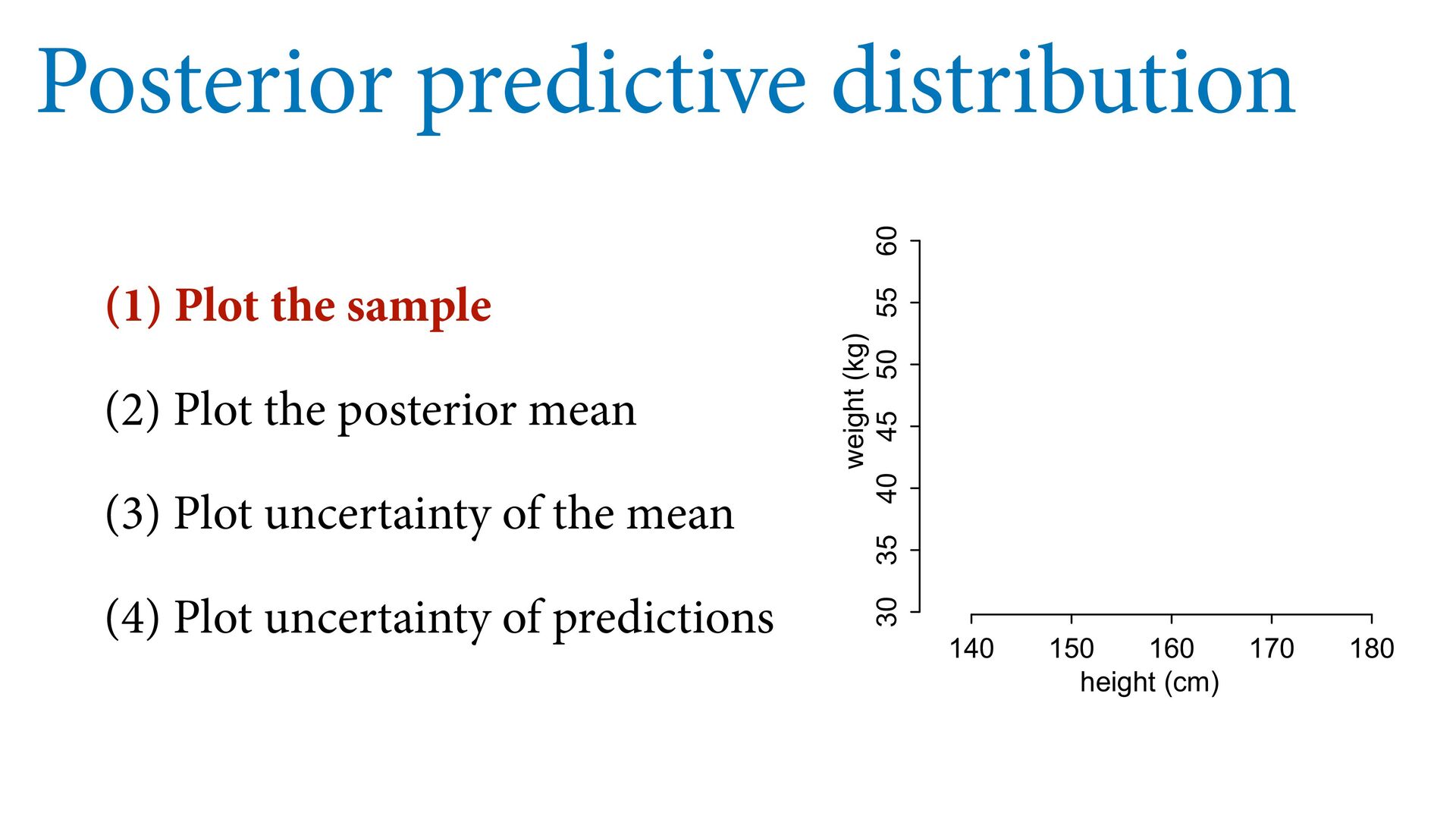
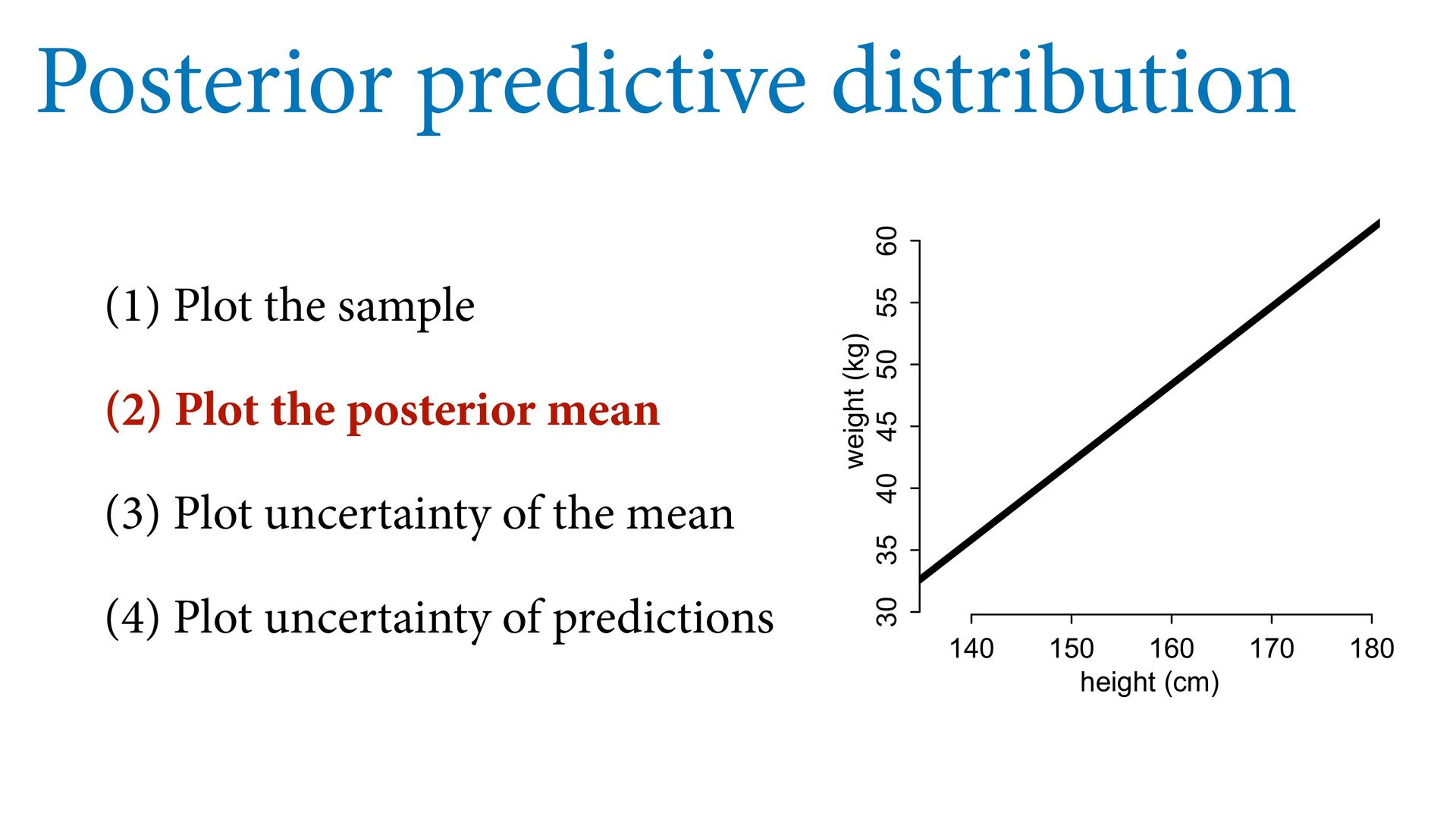
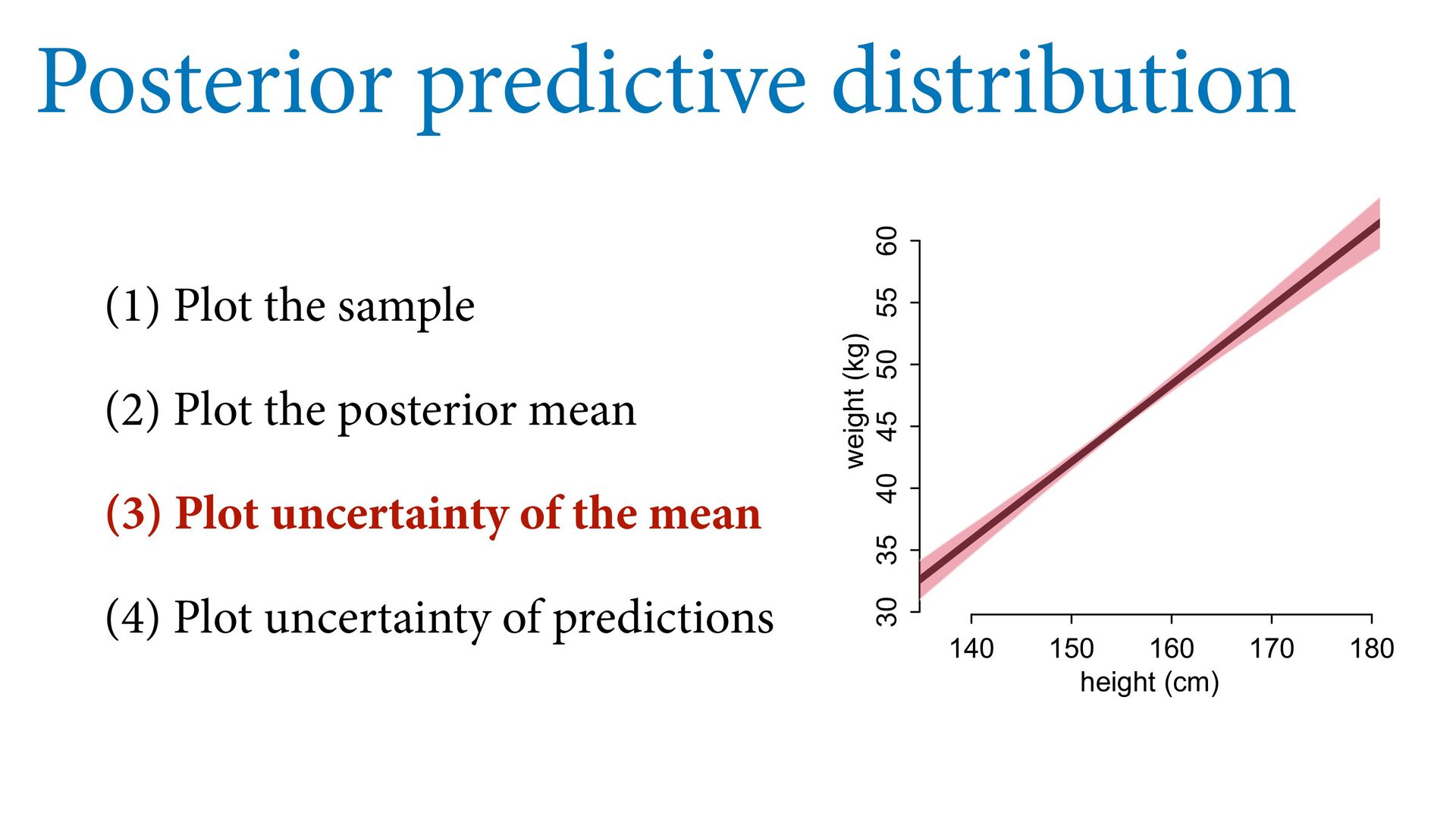
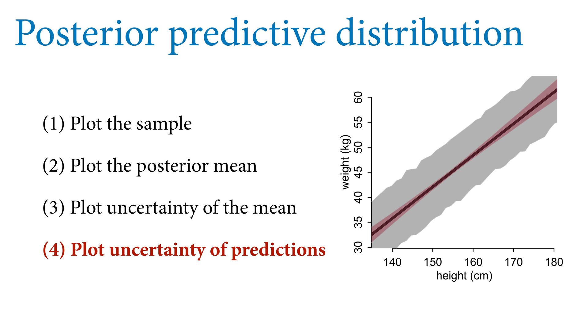
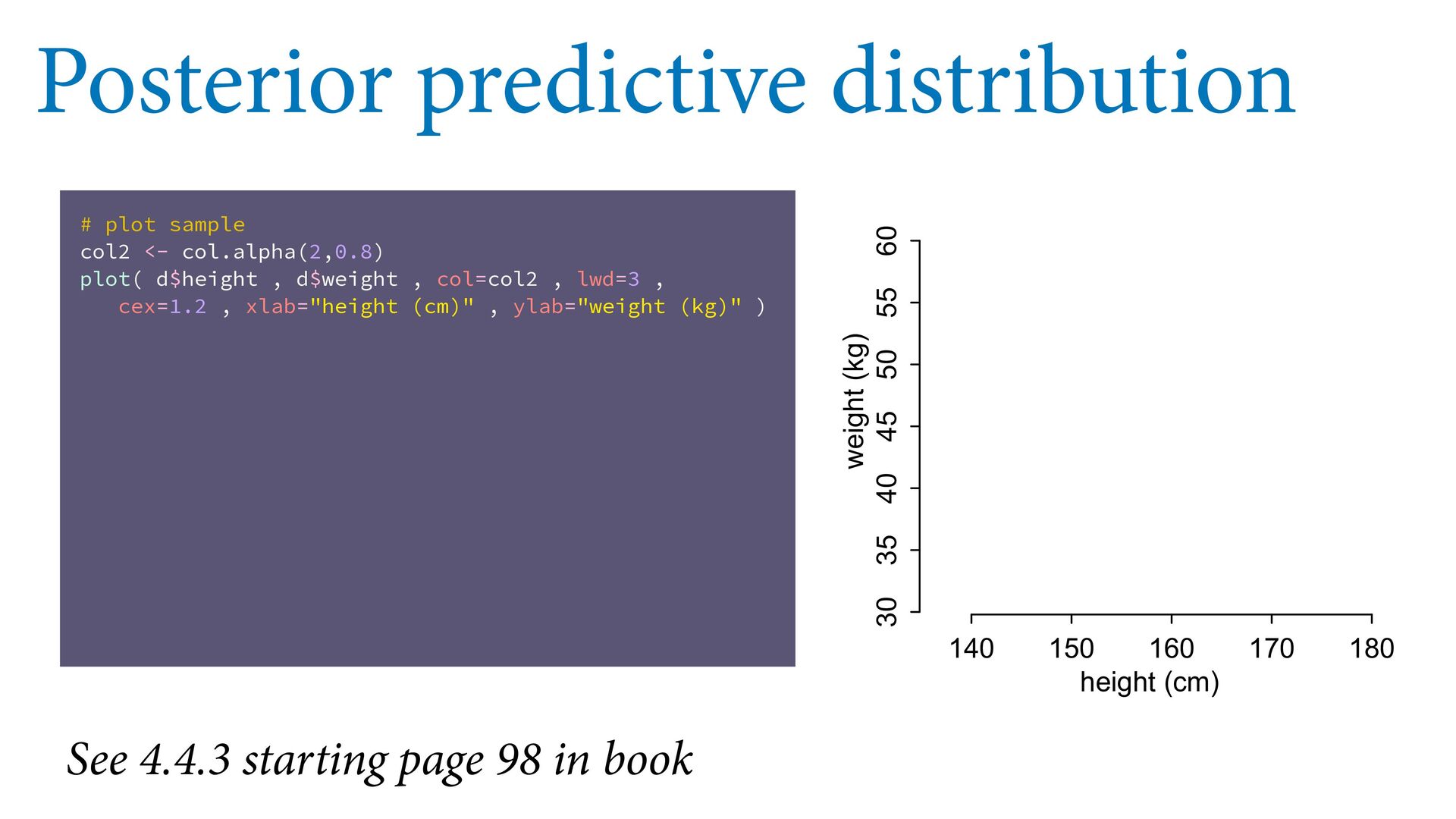
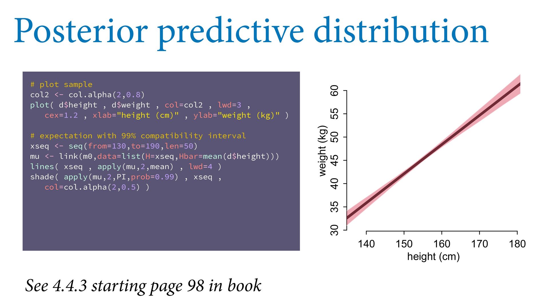
    55 60 height (cm) weight (kg) Posterior predictive distribution # plot sample col2 <- col.alpha(2,0.8) plot( d$height , d$weight , col=col2 , lwd=3 , cex=1.2 , xlab="height (cm)" , ylab="weight (kg)" ) # expectation with 99% compatibility interval xseq <- seq(from=130,to=190,len=50) mu <- link(m0,data=list(H=xseq,Hbar=mean(d$height))) lines( xseq , apply(mu,2,mean) , lwd=4 ) shade( apply(mu,2,PI,prob=0.99) , xseq , col=col.alpha(2,0.5) ) # 89% prediction interval W_sim <- sim(m0,data=list(H=xseq,Hbar=mean(d$height))) shade( apply(W_sim,2,PI,prob=0.89) , xseq , col=col.alpha(1,0.3) ) See 4.4.3 starting page 98 in book
  56. Flexible Linear Thermometers (2) Scientific model How does height influence

    weight? H W W = f(H) “Weight is some function of height” μ i = α + β(H i − ¯ H) W i ∼ Normal(μ i , σ) α ∼ Normal(60,10) β ∼ LogNormal(0,1) σ ∼ Uniform(0,10)
  57. Course Schedule Week 1 Bayesian inference Chapters 1, 2, 3

    Week 2 Linear models & Causal Inference Chapter 4 Week 3 Causes, Confounds & Colliders Chapters 5 & 6 Week 4 Overfitting / Interactions Chapters 7 & 8 Week 5 MCMC & Generalized Linear Models Chapters 9, 10, 11 Week 6 Integers & Other Monsters Chapters 11 & 12 Week 7 Multilevel models I Chapter 13 Week 8 Multilevel models II Chapter 14 Week 9 Measurement & Missingness Chapter 15 Week 10 Generalized Linear Madness Chapter 16 https://github.com/rmcelreath/statrethinking_2022