Statistical Rethinking 2022 Lecture 15

Course materials: https://github.com/rmcelreath/stat_rethinking_2022

Transcript

1. Statistical Rethinking 15: Social Networks 2022
7. What Motivates Sharing? “Up in our country we are human! And since we are human we help each other. We don't like to hear anybody say thanks for that. What I get today you may get tomorrow. Up here we say that by gifts one makes slaves and by whips one makes dogs.” Quoted in Peter Freuchen’s 1961 book about the Inuit Ingrid Vang Nyman
8. data(KosterLeckie) Year of food transfers among 25 households in Arang Dak 25!/(2!(25-2)!) = 300 dyads How much sharing explained by reciprocity? How much by generalized giving? Which dyads? Which households? What Motivates Sharing? Koster & Leckie 2014 Photo: Dr Karl Frost
9. What Motivates Sharing? Koster & Leckie 2014 0 20 40 60 80 100 0 20 40 60 80 100 A gives B B gives A
10. GAB HA HB Household A Household B A gives to B
11. GAB HA HB TAB Household A Household B A gives to B Social “tie” from A to B
12. GAB HA HB TAB Household A Household B Social “tie” from A to B TBA Social “tie” from B to A
13. GAB HA HB TAB Household A Household B Social “tie” from A to B TBA Social “tie” from B to A Wealth A Wealth B Location A Location B Kinship Friendship
14. What Motivates Sharing? TAB and TBA are not observable Social network: Pattern of directed exchange Social networks are abstractions, are not data What is a principled approach? GAB HA HB TAB TBA
15. Figure 1: Dependence structure between Resist Adhockery Hart et al 2021 Common Permutation Methods in Animal Social Network Analysis Do Not Control for Non-independence
16. Drawing the Social Owl (1) Estimand: Reciprocity & what explains it (2) Generative model (3) Statistical model (4) Analyze sample
17. GAB HA HB TAB TBA
18. GAB HA HB TAB TBA Backdoor paths
19. Drawing the Social Owl (1) Estimand: Reciprocity & what explains it (2) Generative model (3) Statistical model (4) Analyze sample
20. GAB HA HB TAB TBA Backdoor paths
21. GAB HA HB TAB TBA
22. # N households N <- 25 dyads <- t(combn(N,2)) N_dyads <- nrow(dyads) # simulate "friendships" in which ties are shared f <- rbern(N_dyads,0.1) # 10% of dyads are friends # now simulate directed ties for all individuals # there can be ties that are not reciprocal alpha <- (-3) # base rate of ties; -3 ~= 0.05 y <- matrix(NA,N,N) # edge list for ( i in 1:N ) for ( j in 1:N ) { if ( i != j ) { # directed tie from i to j ids <- sort( c(i,j) ) the_dyad <- which( dyads[,1]==ids[1] & dyads[,2]==ids[2] ) p_tie <- f[the_dyad] + (1-f[the_dyad])*inv_logit( alpha ) y[i,j] <- rbern( 1 , p_tie ) } }#ij
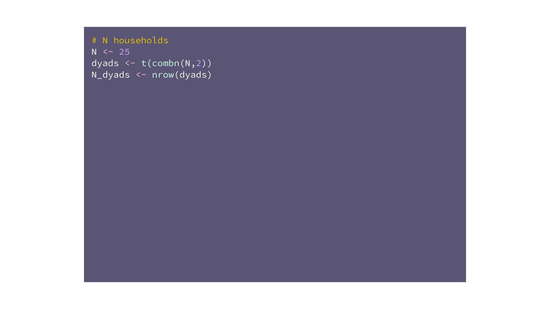
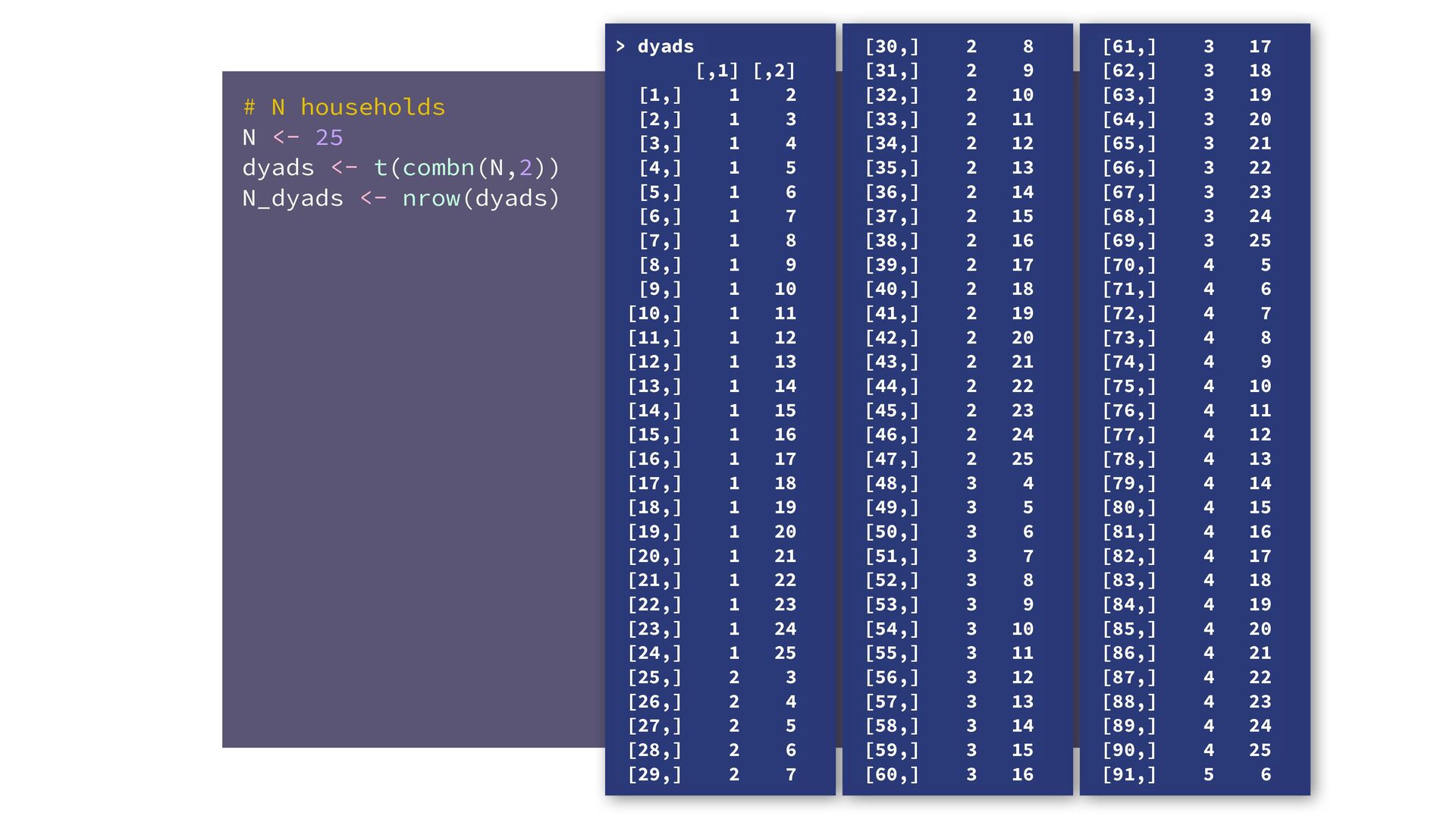
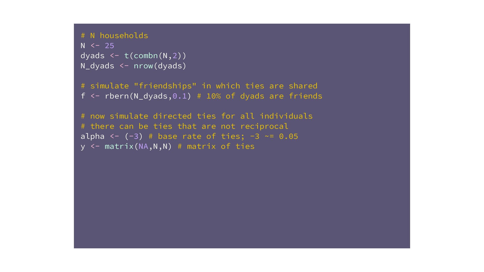
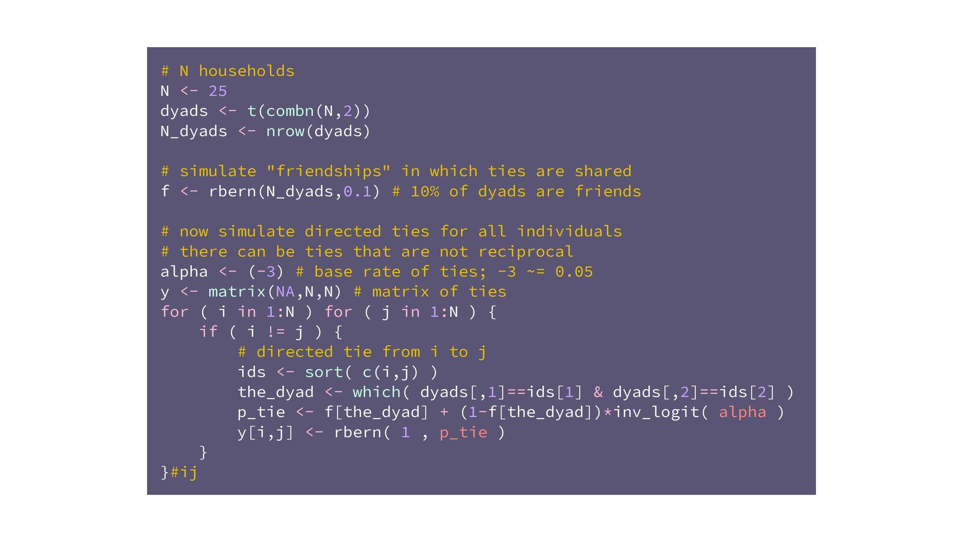
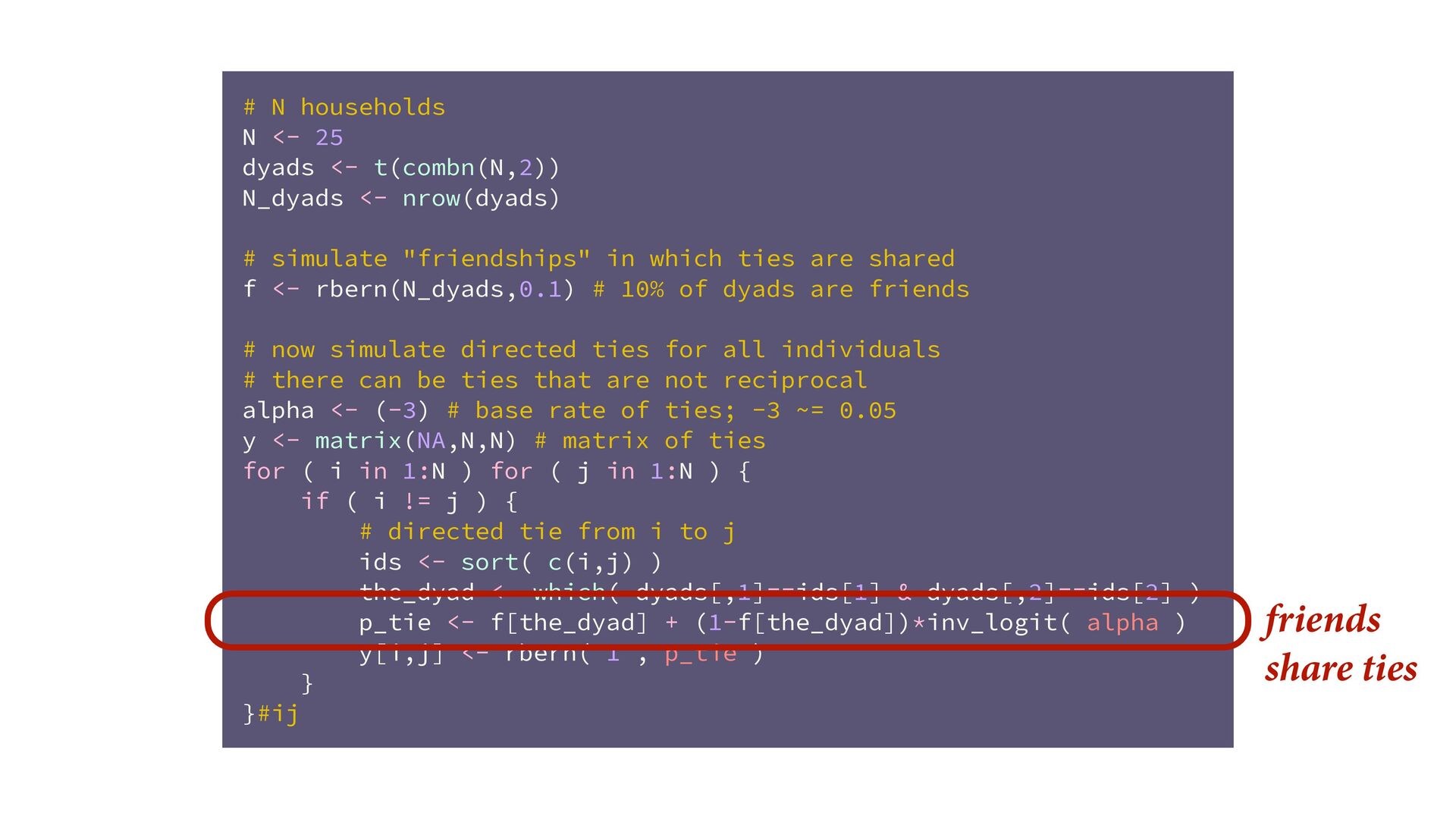
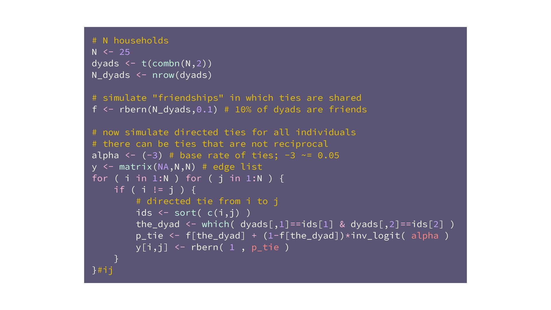
23. # N households N <- 25 dyads <- t(combn(N,2)) N_dyads <- nrow(dyads) # simulate "friendships" in which ties are shared f <- rbern(N_dyads,0.1) # 10% of dyads are friends # now simulate directed ties for all individuals # there can be ties that are not reciprocal alpha <- (-3) # base rate of ties; -3 ~= 0.05 y <- matrix(NA,N,N) # edge list for ( i in 1:N ) for ( j in 1:N ) { if ( i != j ) { # directed tie from i to j ids <- sort( c(i,j) ) the_dyad <- which( dyads[,1]==ids[1] & dyads[,2]==ids[2] ) p_tie <- f[the_dyad] + (1-f[the_dyad])*inv_logit( alpha ) y[i,j] <- rbern( 1 , p_tie ) } }#ij > dyads [,1] [,2] [1,] 1 2 [2,] 1 3 [3,] 1 4 [4,] 1 5 [5,] 1 6 [6,] 1 7 [7,] 1 8 [8,] 1 9 [9,] 1 10 [10,] 1 11 [11,] 1 12 [12,] 1 13 [13,] 1 14 [14,] 1 15 [15,] 1 16 [16,] 1 17 [17,] 1 18 [18,] 1 19 [19,] 1 20 [20,] 1 21 [21,] 1 22 [22,] 1 23 [23,] 1 24 [24,] 1 25 [25,] 2 3 [26,] 2 4 [27,] 2 5 [28,] 2 6 [29,] 2 7 [30,] 2 8 [31,] 2 9 [32,] 2 10 [33,] 2 11 [34,] 2 12 [35,] 2 13 [36,] 2 14 [37,] 2 15 [38,] 2 16 [39,] 2 17 [40,] 2 18 [41,] 2 19 [42,] 2 20 [43,] 2 21 [44,] 2 22 [45,] 2 23 [46,] 2 24 [47,] 2 25 [48,] 3 4 [49,] 3 5 [50,] 3 6 [51,] 3 7 [52,] 3 8 [53,] 3 9 [54,] 3 10 [55,] 3 11 [56,] 3 12 [57,] 3 13 [58,] 3 14 [59,] 3 15 [60,] 3 16 [61,] 3 17 [62,] 3 18 [63,] 3 19 [64,] 3 20 [65,] 3 21 [66,] 3 22 [67,] 3 23 [68,] 3 24 [69,] 3 25 [70,] 4 5 [71,] 4 6 [72,] 4 7 [73,] 4 8 [74,] 4 9 [75,] 4 10 [76,] 4 11 [77,] 4 12 [78,] 4 13 [79,] 4 14 [80,] 4 15 [81,] 4 16 [82,] 4 17 [83,] 4 18 [84,] 4 19 [85,] 4 20 [86,] 4 21 [87,] 4 22 [88,] 4 23 [89,] 4 24 [90,] 4 25 [91,] 5 6
24. # N households N <- 25 dyads <- t(combn(N,2)) N_dyads <- nrow(dyads) # simulate "friendships" in which ties are shared f <- rbern(N_dyads,0.1) # 10% of dyads are friends # now simulate directed ties for all individuals # there can be ties that are not reciprocal alpha <- (-3) # base rate of ties; -3 ~= 0.05 y <- matrix(NA,N,N) # edge list for ( i in 1:N ) for ( j in 1:N ) { if ( i != j ) { # directed tie from i to j ids <- sort( c(i,j) ) the_dyad <- which( dyads[,1]==ids[1] & dyads[,2]==ids[2] ) p_tie <- f[the_dyad] + (1-f[the_dyad])*inv_logit( alpha ) y[i,j] <- rbern( 1 , p_tie ) } }#ij
25. # N households N <- 25 dyads <- t(combn(N,2)) N_dyads <- nrow(dyads) # simulate "friendships" in which ties are shared f <- rbern(N_dyads,0.1) # 10% of dyads are friends # now simulate directed ties for all individuals # there can be ties that are not reciprocal alpha <- (-3) # base rate of ties; -3 ~= 0.05 y <- matrix(NA,N,N) # matrix of ties for ( i in 1:N ) for ( j in 1:N ) { if ( i != j ) { # directed tie from i to j ids <- sort( c(i,j) ) the_dyad <- which( dyads[,1]==ids[1] & dyads[,2]==ids[2] ) p_tie <- f[the_dyad] + (1-f[the_dyad])*inv_logit( alpha ) y[i,j] <- rbern( 1 , p_tie ) } }#ij
26. # N households N <- 25 dyads <- t(combn(N,2)) N_dyads <- nrow(dyads) # simulate "friendships" in which ties are shared f <- rbern(N_dyads,0.1) # 10% of dyads are friends # now simulate directed ties for all individuals # there can be ties that are not reciprocal alpha <- (-3) # base rate of ties; -3 ~= 0.05 y <- matrix(NA,N,N) # matrix of ties for ( i in 1:N ) for ( j in 1:N ) { if ( i != j ) { # directed tie from i to j ids <- sort( c(i,j) ) the_dyad <- which( dyads[,1]==ids[1] & dyads[,2]==ids[2] ) p_tie <- f[the_dyad] + (1-f[the_dyad])*inv_logit( alpha ) y[i,j] <- rbern( 1 , p_tie ) } }#ij
27. # N households N <- 25 dyads <- t(combn(N,2)) N_dyads <- nrow(dyads) # simulate "friendships" in which ties are shared f <- rbern(N_dyads,0.1) # 10% of dyads are friends # now simulate directed ties for all individuals # there can be ties that are not reciprocal alpha <- (-3) # base rate of ties; -3 ~= 0.05 y <- matrix(NA,N,N) # matrix of ties for ( i in 1:N ) for ( j in 1:N ) { if ( i != j ) { # directed tie from i to j ids <- sort( c(i,j) ) the_dyad <- which( dyads[,1]==ids[1] & dyads[,2]==ids[2] ) p_tie <- f[the_dyad] + (1-f[the_dyad])*inv_logit( alpha ) y[i,j] <- rbern( 1 , p_tie ) } }#ij friends share ties
28. # now simulate gifts giftsAB <- rep(NA,N_dyads) giftsBA <- rep(NA,N_dyads) lambda <- log(c(0.5,2)) # rates of giving for y=0,y=1 for ( i in 1:N_dyads ) { A <- dyads[i,1] B <- dyads[i,2] giftsAB[i] <- rpois( 1 , exp( lambda[1+y[A,B]] ) ) giftsBA[i] <- rpois( 1 , exp( lambda[1+y[B,A]] ) ) }
29. # now simulate gifts giftsAB <- rep(NA,N_dyads) giftsBA <- rep(NA,N_dyads) lambda <- log(c(0.5,2)) # rates of giving for y=0,y=1 for ( i in 1:N_dyads ) { A <- dyads[i,1] B <- dyads[i,2] giftsAB[i] <- rpois( 1 , exp( lambda[1+y[A,B]] ) ) giftsBA[i] <- rpois( 1 , exp( lambda[1+y[B,A]] ) ) } # draw network library(igraph) sng <- graph_from_adjacency_matrix(y) lx <- layout_nicely(sng) vcol <- "#DE536B" plot(sng , layout=lx , vertex.size=8 , edge.arrow.size=0.75 , edge.width=2 , edge.curved=0.35 , vertex.color=vcol , edge.color=grau() , asp=0.9 , margin = -0.05 , vertex.label=NA )
30. Drawing the Social Owl (1) Estimand: Reciprocity & what explains it (2) Generative model (3) Statistical model (4) Analyze sample
31. G AB ∼ Poisson(λ AB ) log(λ AB ) = α + T AB Gifts A to B average Tie A to B
32. G AB ∼ Poisson(λ AB ) G BA ∼ Poisson(λ BA ) log(λ AB ) = α + T AB log(λ BA ) = α + T BA Gifts A to B Gifts B to A average Tie A to B Tie B to A
33. G AB ∼ Poisson(λ AB ) G BA ∼ Poisson(λ BA ) log(λ AB ) = α + T AB log(λ BA ) = α + T BA ( T AB T BA ) ∼ MVNormal [ 0 0] , [ σ2 ρσ2 ρσ2 σ2 ] covariance within dyads variance among ties The AB dyad
34. G AB ∼ Poisson(λ AB ) G BA ∼ Poisson(λ BA ) log(λ AB ) = α + T AB log(λ BA ) = α + T BA ( T AB T BA ) ∼ MVNormal [ 0 0] , [ σ2 ρσ2 ρσ2 σ2 ] ρ ∼ LKJCorr(2) σ ∼ Exponential(1) partial pooling for network ties α ∼ Normal(0,1)
35. # dyad model f_dyad <- alist( GAB ~ poisson( lambdaAB ), GBA ~ poisson( lambdaBA ), log(lambdaAB) <- a + T[D,1] , log(lambdaBA) <- a + T[D,2] , a ~ normal(0,1), ## dyad effects transpars> matrix[N_dyads,2]:T <- compose_noncentered( rep_vector(sigma_T,2) , L_Rho_T , Z ), matrix[2,N_dyads]:Z ~ normal( 0 , 1 ), cholesky_factor_corr[2]:L_Rho_T ~ lkj_corr_cholesky( 2 ), sigma_T ~ exponential(1), ## compute correlation matrix for dyads gq> matrix[2,2]:Rho_T <<- Chol_to_Corr( L_Rho_T ) ) mGD <- ulam( f_dyad , data=sim_data , chains=4 , cores=4 , iter=2000 )
36. # dyad model f_dyad <- alist( GAB ~ poisson( lambdaAB ), GBA ~ poisson( lambdaBA ), log(lambdaAB) <- a + T[D,1] , log(lambdaBA) <- a + T[D,2] , a ~ normal(0,1), ## dyad effects transpars> matrix[N_dyads,2]:T <- compose_noncentered( rep_vector(sigma_T,2) , L_Rho_T , Z ), matrix[2,N_dyads]:Z ~ normal( 0 , 1 ), cholesky_factor_corr[2]:L_Rho_T ~ lkj_corr_cholesky( 2 ), sigma_T ~ exponential(1), ## compute correlation matrix for dyads gq> matrix[2,2]:Rho_T <<- Chol_to_Corr( L_Rho_T ) ) mGD <- ulam( f_dyad , data=sim_data , chains=4 , cores=4 , iter=2000 ) ( T AB T BA ) ∼ MVNormal [ 0 0] , [ σ2 ρσ2 ρσ2 σ2 ]
37. n_eff = 6334 T[15,1] n_eff = 9318 T[16,1] n_eff = 9272 T[17,1] n_eff = 9187 T[18,1] n_eff = 8481 T[19,1] n_eff = 7697 T[20,1] n_eff = 8645 T[21,1] n_eff = 8777 T[22,1] n_eff = 7968 T[23,1] n_eff = 7488 T[24,1] n_eff = 7282 T[25,1] n_eff = 7767 T[26,1] n_eff = 8068 T[27,1] n_eff = 9159 T[28,1] n_eff = 9809 T[29,1] n_eff = 8239 T[30,1] n_eff = 8984 T[31,1] n_eff = 8389 T[32,1] n_eff = 6304 T[33,1] n_eff = 8794 T[34,1]
38. Posterior ties no tie tie -0.5 0.0 0.5 1.0 1.5 0 1 2 3 4 posterior mean T Density -1.0 -0.5 0.0 0.5 1.0 0.0 0.5 1.0 1.5 2.0 correlation within dyads Density
39. Posterior ties friends -0.2 0.0 0.2 0.4 0.6 0.8 -0.2 0.2 0.6 1.0 Household A Household B -1.0 -0.5 0.0 0.5 1.0 0.0 0.5 1.0 1.5 2.0 correlation within dyads Density
40. Drawing the Social Owl (1) Estimand: Reciprocity & what explains it (2) Generative model (3) Statistical model (4) Analyze sample -0.2 0.0 0.2 0.4 0.6 0.8 -0.2 0.2 0.6 1.0 Household A Household B
41. # analyze sample kl_data <- list( N_dyads = nrow(kl_dyads), N_households = max(kl_dyads$hidB), D = 1:nrow(kl_dyads), HA = kl_dyads$hidA, HB = kl_dyads$hidB, GAB = kl_dyads$giftsAB, GBA = kl_dyads$giftsBA ) mGDkl <- ulam( f_dyad , data=kl_data , chains=4 , cores=4 , iter=2000 ) precis( mGDkl , depth=3 , pars=c("a","Rho_T","sigma_T") )
42. # analyze sample kl_data <- list( N_dyads = nrow(kl_dyads), N_households = max(kl_dyads$hidB), D = 1:nrow(kl_dyads), HA = kl_dyads$hidA, HB = kl_dyads$hidB, GAB = kl_dyads$giftsAB, GBA = kl_dyads$giftsBA ) mGDkl <- ulam( f_dyad , data=kl_data , chains=4 , cores=4 , iter=2000 ) precis( mGDkl , depth=3 , pars=c("a","Rho_T","sigma_T") ) mean sd 5.5% 94.5% n_eff Rhat4 a 0.55 0.08 0.42 0.68 2246 1.00 Rho_T[1,1] 1.00 0.00 1.00 1.00 NaN NaN Rho_T[1,2] 0.35 0.07 0.24 0.45 1351 1.00 Rho_T[2,1] 0.35 0.07 0.24 0.45 1351 1.00 Rho_T[2,2] 1.00 0.00 1.00 1.00 NaN NaN sigma_T 1.44 0.06 1.35 1.55 1249 1.01 -1.0 -0.5 0.0 0.5 1.0 0 1 2 3 4 5 6 correlation within dyads Density
43. GAB HA HB TAB TBA Backdoor paths
44. PAUSE
45. Drawing the Social Owl (1) Estimand: Reciprocity & what explains it (2) Generative model (3) Statistical model (4) Analyze sample GAB HA HB TAB TBA Effect of ties Effect of general household traits
46. # N households N <- 25 dyads <- t(combn(N,2)) N_dyads <- nrow(dyads) # simulate "friendships" in which ties are shared f <- rbern(N_dyads,0.1) # 10% of dyads are friends # now simulate directed ties for all individuals # there can be ties that are not reciprocal alpha <- (-3) # base rate of ties; -3 ~= 0.05 y <- matrix(NA,N,N) # edge list for ( i in 1:N ) for ( j in 1:N ) { if ( i != j ) { # directed tie from i to j ids <- sort( c(i,j) ) the_dyad <- which( dyads[,1]==ids[1] & dyads[,2]==ids[2] ) p_tie <- f[the_dyad] + (1-f[the_dyad])*inv_logit( alpha ) y[i,j] <- rbern( 1 , p_tie ) } }#ij
47. # simulate wealth W <- rnorm(N) # standardized relative wealth in community bWG <- 0.5 # effect of wealth on giving - rich give more bWR <- (-1) # effect of wealth on receiving - rich get less / poor get more # now simulate gifts giftsAB <- rep(NA,N_dyads) giftsBA <- rep(NA,N_dyads) lambda <- log(c(0.5,2)) # rates of giving for y=0,y=1 for ( i in 1:N_dyads ) { A <- dyads[i,1] B <- dyads[i,2] giftsAB[i] <- rpois( 1 , exp( lambda[1+y[A,B]] + bWG*W[A] + bWR*W[B] ) ) giftsBA[i] <- rpois( 1 , exp( lambda[1+y[B,A]] + bWG*W[B] + bWR*W[A] ) ) }
48. # simulate wealth W <- rnorm(N) # standardized relative wealth in community bWG <- 0.5 # effect of wealth on giving - rich give more bWR <- (-1) # effect of wealth on receiving - rich get less / poor get more # now simulate gifts giftsAB <- rep(NA,N_dyads) giftsBA <- rep(NA,N_dyads) lambda <- log(c(0.5,2)) # rates of giving for y=0,y=1 for ( i in 1:N_dyads ) { A <- dyads[i,1] B <- dyads[i,2] giftsAB[i] <- rpois( 1 , exp( lambda[1+y[A,B]] + bWG*W[A] + bWR*W[B] ) ) giftsBA[i] <- rpois( 1 , exp( lambda[1+y[B,A]] + bWG*W[B] + bWR*W[A] ) ) }
49. G AB ∼ Poisson(λ AB ) G BA ∼ Poisson(λ BA ) log(λ AB ) = α + T AB log(λ BA ) = α + T BA ( T AB T BA ) ∼ MVNormal [ 0 0] , [ σ2 ρσ2 ρσ2 σ2 ] ρ ∼ LKJCorr(2) σ ∼ Exponential(1) α ∼ Normal(0,1)
50. G AB ∼ Poisson(λ AB ) G BA ∼ Poisson(λ BA ) log(λ AB ) = α + T AB log(λ BA ) = α + T BA ( T AB T BA ) ∼ MVNormal [ 0 0] , [ σ2 ρσ2 ρσ2 σ2 ] ρ ∼ LKJCorr(2) σ ∼ Exponential(1) α ∼ Normal(0,1)
51. G AB ∼ Poisson(λ AB ) G BA ∼ Poisson(λ BA ) log(λ AB ) = α + T AB log(λ BA ) = α + T BA ( T AB T BA ) ∼ MVNormal [ 0 0] , [ σ2 ρσ2 ρσ2 σ2 ] ρ ∼ LKJCorr(2) σ ∼ Exponential(1) α ∼ Normal(0,1)
52. log(λ AB ) = α + T AB + G A + R B G AB ∼ Poisson(λ AB ) G BA ∼ Poisson(λ BA ) log(λ AB ) = α + T AB log(λ BA ) = α + T BA ( T AB T BA ) ∼ MVNormal [ 0 0] , [ σ2 ρσ2 ρσ2 σ2 ] ρ ∼ LKJCorr(2) σ ∼ Exponential(1) α ∼ Normal(0,1)
53. log(λ AB ) = α + T AB + G A + R B G AB ∼ Poisson(λ AB ) G BA ∼ Poisson(λ BA ) log(λ BA ) = α + T BA + G B + R A ( T AB T BA ) ∼ MVNormal [ 0 0] , [ σ2 ρσ2 ρσ2 σ2 ] ρ ∼ LKJCorr(2) σ ∼ Exponential(1) α ∼ Normal(0,1)
54. log(λ AB ) = α + T AB + G A + R B G AB ∼ Poisson(λ AB ) G BA ∼ Poisson(λ BA ) log(λ BA ) = α + T BA + G B + R A ( T AB T BA ) ∼ MVNormal [ 0 0] , [ σ2 ρσ2 ρσ2 σ2 ] ρ ∼ LKJCorr(2) σ ∼ Exponential(1) α ∼ Normal(0,1) ( G A R A ) ∼ MVNormal [ 0 0] , [ σ2 G rσ G σ R rσ G σ R σ2 R ]
55. log(λ AB ) = α + T AB + G A + R B G AB ∼ Poisson(λ AB ) G BA ∼ Poisson(λ BA ) log(λ BA ) = α + T BA + G B + R A ( T AB T BA ) ∼ MVNormal [ 0 0] , [ σ2 ρσ2 ρσ2 σ2 ] ρ ∼ LKJCorr(2) σ ∼ Exponential(1) α ∼ Normal(0,1) ( G A R A ) ∼ MVNormal [ 0 0] , [ σ2 G rσ G σ R rσ G σ R σ2 R ] A’s giving & receiving Covariance matrix of household giving & receiving
56. log(λ AB ) = α + T AB + G A + R B G AB ∼ Poisson(λ AB ) G BA ∼ Poisson(λ BA ) log(λ BA ) = α + T BA + G B + R A ( T AB T BA ) ∼ MVNormal [ 0 0] , [ σ2 ρσ2 ρσ2 σ2 ] ρ ∼ LKJCorr(2) σ ∼ Exponential(1) α ∼ Normal(0,1) ( G A R A ) ∼ MVNormal ([ 0 0] , R GR , S GR ) A’s giving & receiving Correlation matrix Standard
 deviations
57. log(λ AB ) = α + T AB + G A + R B G AB ∼ Poisson(λ AB ) G BA ∼ Poisson(λ BA ) log(λ BA ) = α + T BA + G B + R A ( T AB T BA ) ∼ MVNormal [ 0 0] , [ σ2 ρσ2 ρσ2 σ2 ] ρ ∼ LKJCorr(2) σ ∼ Exponential(1) α ∼ Normal(0,1) ( G A R A ) ∼ MVNormal ([ 0 0] , R GR , S GR ) R GR ∼ LKJCorr(2) S GR ∼ Exponential(1)
58. log(λ AB ) = α + T AB + G A + R B G AB ∼ Poisson(λ AB ) G BA ∼ Poisson(λ BA ) log(λ BA ) = α + T BA + G B + R A ( T AB T BA ) ∼ MVNormal [ 0 0] , [ σ2 ρσ2 ρσ2 σ2 ] ρ ∼ LKJCorr(2) σ ∼ Exponential(1) α ∼ Normal(0,1) ( G A R A ) ∼ MVNormal ([ 0 0] , R GR , S GR ) R GR ∼ LKJCorr(2) S GR ∼ Exponential(1) 602 social network parameters 53 household parameters 25 households 
 300 dyads 
 600 gift observations
59. # general model f_general <- alist( GAB ~ poisson( lambdaAB ), GBA ~ poisson( lambdaBA ), log(lambdaAB) <- a + T[D,1] + gr[HA,1] + gr[HB,2], log(lambdaBA) <- a + T[D,2] + gr[HB,1] + gr[HA,2], a ~ normal(0,1), ## dyad effects - non-centered transpars> matrix[N_dyads,2]:T <- compose_noncentered(rep_vector(sigma_T,2),L_Rho_T,Z), matrix[2,N_dyads]:Z ~ normal( 0 , 1 ), cholesky_factor_corr[2]:L_Rho_T ~ lkj_corr_cholesky( 2 ), sigma_T ~ exponential(1), ## gr matrix of varying effects transpars> matrix[N_households,2]:gr <- compose_noncentered( sigma_gr , L_Rho_gr , Zgr ), matrix[2,N_households]:Zgr ~ normal( 0 , 1 ), cholesky_factor_corr[2]:L_Rho_gr ~ lkj_corr_cholesky( 2 ), vector[2]:sigma_gr ~ exponential(1), ## compute correlation matrixes gq> matrix[2,2]:Rho_T <<- Chol_to_Corr( L_Rho_T ), gq> matrix[2,2]:Rho_gr <<- Chol_to_Corr( L_Rho_gr ) ) mGDGR <- ulam(f_general,data=sim_data,chains=4,cores=4,iter=2000) log(λ AB ) = α + T AB + G A + R B G AB ∼ Poisson(λ AB ) G BA ∼ Poisson(λ BA ) log(λ BA ) = α + T BA + G B + R A ( T AB T BA ) ∼ MVNormal [ 0 0] , [ σ2 ρσ2 ρσ2 σ2 ] ρ ∼ LKJCorr(2) σ ∼ Exponential(1) α ∼ Normal(0,1) ( G A R A ) ∼ MVNormal ([ 0 0] , R GR , S GR ) R GR ∼ LKJCorr(2) S GR ∼ Exponential(1)
60. # general model f_general <- alist( GAB ~ poisson( lambdaAB ), GBA ~ poisson( lambdaBA ), log(lambdaAB) <- a + T[D,1] + gr[HA,1] + gr[HB,2], log(lambdaBA) <- a + T[D,2] + gr[HB,1] + gr[HA,2], a ~ normal(0,1), ## dyad effects - non-centered transpars> matrix[N_dyads,2]:T <- compose_noncentered(rep_vector(sigma_T,2),L_Rho_T,Z), matrix[2,N_dyads]:Z ~ normal( 0 , 1 ), cholesky_factor_corr[2]:L_Rho_T ~ lkj_corr_cholesky( 2 ), sigma_T ~ exponential(1), ## gr matrix of varying effects transpars> matrix[N_households,2]:gr <- compose_noncentered( sigma_gr , L_Rho_gr , Zgr ), matrix[2,N_households]:Zgr ~ normal( 0 , 1 ), cholesky_factor_corr[2]:L_Rho_gr ~ lkj_corr_cholesky( 2 ), vector[2]:sigma_gr ~ exponential(1), ## compute correlation matrixes gq> matrix[2,2]:Rho_T <<- Chol_to_Corr( L_Rho_T ), gq> matrix[2,2]:Rho_gr <<- Chol_to_Corr( L_Rho_gr ) ) mGDGR <- ulam(f_general,data=sim_data,chains=4,cores=4,iter=2000) log(λ AB ) = α + T AB + G A + R B G AB ∼ Poisson(λ AB ) G BA ∼ Poisson(λ BA ) log(λ BA ) = α + T BA + G B + R A ( T AB T BA ) ∼ MVNormal [ 0 0] , [ σ2 ρσ2 ρσ2 σ2 ] ρ ∼ LKJCorr(2) σ ∼ Exponential(1) α ∼ Normal(0,1) ( G A R A ) ∼ MVNormal ([ 0 0] , R GR , S GR ) R GR ∼ LKJCorr(2) S GR ∼ Exponential(1)
61. # general model f_general <- alist( GAB ~ poisson( lambdaAB ), GBA ~ poisson( lambdaBA ), log(lambdaAB) <- a + T[D,1] + gr[HA,1] + gr[HB,2], log(lambdaBA) <- a + T[D,2] + gr[HB,1] + gr[HA,2], a ~ normal(0,1), ## dyad effects - non-centered transpars> matrix[N_dyads,2]:T <- compose_noncentered(rep_vector(sigma_T,2),L_Rho_T,Z), matrix[2,N_dyads]:Z ~ normal( 0 , 1 ), cholesky_factor_corr[2]:L_Rho_T ~ lkj_corr_cholesky( 2 ), sigma_T ~ exponential(1), ## gr matrix of varying effects transpars> matrix[N_households,2]:gr <- compose_noncentered( sigma_gr , L_Rho_gr , Zgr ), matrix[2,N_households]:Zgr ~ normal( 0 , 1 ), cholesky_factor_corr[2]:L_Rho_gr ~ lkj_corr_cholesky( 2 ), vector[2]:sigma_gr ~ exponential(1), ## compute correlation matrixes gq> matrix[2,2]:Rho_T <<- Chol_to_Corr( L_Rho_T ), gq> matrix[2,2]:Rho_gr <<- Chol_to_Corr( L_Rho_gr ) ) mGDGR <- ulam(f_general,data=sim_data,chains=4,cores=4,iter=2000) log(λ AB ) = α + T AB + G A + R B G AB ∼ Poisson(λ AB ) G BA ∼ Poisson(λ BA ) log(λ BA ) = α + T BA + G B + R A ( T AB T BA ) ∼ MVNormal [ 0 0] , [ σ2 ρσ2 ρσ2 σ2 ] ρ ∼ LKJCorr(2) σ ∼ Exponential(1) α ∼ Normal(0,1) ( G A R A ) ∼ MVNormal ([ 0 0] , R GR , S GR ) R GR ∼ LKJCorr(2) S GR ∼ Exponential(1)
62. # general model f_general <- alist( GAB ~ poisson( lambdaAB ), GBA ~ poisson( lambdaBA ), log(lambdaAB) <- a + T[D,1] + gr[HA,1] + gr[HB,2], log(lambdaBA) <- a + T[D,2] + gr[HB,1] + gr[HA,2], a ~ normal(0,1), ## dyad effects - non-centered transpars> matrix[N_dyads,2]:T <- compose_noncentered(rep_vector(sigma_T,2),L_Rho_T,Z), matrix[2,N_dyads]:Z ~ normal( 0 , 1 ), cholesky_factor_corr[2]:L_Rho_T ~ lkj_corr_cholesky( 2 ), sigma_T ~ exponential(1), ## gr matrix of varying effects transpars> matrix[N_households,2]:gr <- compose_noncentered( sigma_gr , L_Rho_gr , Zgr ), matrix[2,N_households]:Zgr ~ normal( 0 , 1 ), cholesky_factor_corr[2]:L_Rho_gr ~ lkj_corr_cholesky( 2 ), vector[2]:sigma_gr ~ exponential(1), ## compute correlation matrixes gq> matrix[2,2]:Rho_T <<- Chol_to_Corr( L_Rho_T ), gq> matrix[2,2]:Rho_gr <<- Chol_to_Corr( L_Rho_gr ) ) mGDGR <- ulam(f_general,data=sim_data,chains=4,cores=4,iter=2000) log(λ AB ) = α + T AB + G A + R B G AB ∼ Poisson(λ AB ) G BA ∼ Poisson(λ BA ) log(λ BA ) = α + T BA + G B + R A ( T AB T BA ) ∼ MVNormal [ 0 0] , [ σ2 ρσ2 ρσ2 σ2 ] ρ ∼ LKJCorr(2) σ ∼ Exponential(1) α ∼ Normal(0,1) ( G A R A ) ∼ MVNormal ([ 0 0] , R GR , S GR ) R GR ∼ LKJCorr(2) S GR ∼ Exponential(1)
63. 0.0 0.5 1.0 1.5 2.0 2.5 3.0 0.0 0.5 1.0 1.5 2.0 2.5 3.0 generalized giving generalized receiving Synthetic data (validation) households -1.0 -0.5 0.0 0.5 1.0 0 1 2 3 4 correlation giving-receiving Density give-receive
64. 0.0 0.5 1.0 1.5 2.0 2.5 3.0 0.0 0.5 1.0 1.5 2.0 2.5 3.0 generalized giving generalized receiving Synthetic data (validation) -1.0 0.0 1.0 2.0 0.0 0.5 1.0 1.5 posterior mean T Density -0.5 0.0 0.5 1.0 1.5 -0.5 0.0 0.5 1.0 Household A Household B -1.0 -0.5 0.0 0.5 1.0 0.0 1.0 2.0 correlation within dyads Density -1.0 -0.5 0.0 0.5 1.0 0 1 2 3 4 correlation giving-receiving Density households no tie tie reciprocity give-receive friends
65. 0 2 4 6 0 2 4 6 generalized giving generalized receiving Real data (analysis) households reciprocity give-receive dyadic ties -2 -1 0 1 2 3 -2 -1 0 1 2 3 Household A Household B -1.0 -0.5 0.0 0.5 1.0 0 5 10 15 correlation within dyads Density -1.0 -0.5 0.0 0.5 1.0 0.0 0.5 1.0 1.5 2.0 correlation giving-receiving Density
66. Posterior mean network
67. Posterior mean network Samples from posterior Network is uncertain, so all network statistics are uncertain!
68. Social Networks Don’t Exist Varying effects are placeholders Can model the network ties (using dyad features) Can model the giving/receiving (using household features) Relationships can cause other relationships 0 2 4 6 0 2 4 6 generalized giving generalized receiving
69. log(λ AB ) = α + T AB + G A + R B G AB ∼ Poisson(λ AB ) G BA ∼ Poisson(λ BA ) log(λ BA ) = α + T BA + G B + R A ( T AB T BA ) ∼ MVNormal [ 0 0] , [ σ2 ρσ2 ρσ2 σ2 ] ρ ∼ LKJCorr(2) σ ∼ Exponential(1) α ∼ Normal(0,1) ( G A R A ) ∼ MVNormal ([ 0 0] , R GR , S GR ) R GR ∼ LKJCorr(2) S GR ∼ Exponential(1)
70. log(λ AB ) = α + T AB + G A + R B G AB ∼ Poisson(λ AB ) G BA ∼ Poisson(λ BA ) log(λ BA ) = α + T BA + G B + R A ( T AB T BA ) ∼ MVNormal [ 0 0] , [ σ2 ρσ2 ρσ2 σ2 ] ρ ∼ LKJCorr(2) σ ∼ Exponential(1) α ∼ Normal(0,1) ( G A R A ) ∼ MVNormal ([ 0 0] , R GR , S GR ) R GR ∼ LKJCorr(2) S GR ∼ Exponential(1)
71. log(λ AB ) = α + AB + A + ℛ B G AB ∼ Poisson(λ AB ) G BA ∼ Poisson(λ BA ) log(λ BA ) = α + T BA + G B + R A ( T AB T BA ) ∼ MVNormal [ 0 0] , [ σ2 ρσ2 ρσ2 σ2 ] ρ ∼ LKJCorr(2) σ ∼ Exponential(1) α ∼ Normal(0,1) ( G A R A ) ∼ MVNormal ([ 0 0] , R GR , S GR ) R GR ∼ LKJCorr(2) S GR ∼ Exponential(1) AB = T AB + β A A AB linear model for tie strength AB AB varying effect effect of association between A&B
72. log(λ AB ) = α + AB + A + ℛ B G AB ∼ Poisson(λ AB ) G BA ∼ Poisson(λ BA ) log(λ BA ) = α + T BA + G B + R A ( T AB T BA ) ∼ MVNormal [ 0 0] , [ σ2 ρσ2 ρσ2 σ2 ] ρ ∼ LKJCorr(2) σ ∼ Exponential(1) α ∼ Normal(0,1) ( G A R A ) ∼ MVNormal ([ 0 0] , R GR , S GR ) R GR ∼ LKJCorr(2) S GR ∼ Exponential(1) AB = T AB + β A A AB A = G A + β W,G W A A A linear model for giving varying effect effect of A’s wealth on giving
73. log(λ AB ) = α + AB + A + ℛ B G AB ∼ Poisson(λ AB ) G BA ∼ Poisson(λ BA ) log(λ BA ) = α + T BA + G B + R A ( T AB T BA ) ∼ MVNormal [ 0 0] , [ σ2 ρσ2 ρσ2 σ2 ] ρ ∼ LKJCorr(2) σ ∼ Exponential(1) α ∼ Normal(0,1) ( G A R A ) ∼ MVNormal ([ 0 0] , R GR , S GR ) R GR ∼ LKJCorr(2) S GR ∼ Exponential(1) AB = T AB + β A A AB A = G A + β W,G W A ℛ B = R B + β W,R W B ℛ B ℛ B linear model for receiving varying effect effect of B’s wealth on receiving
74. G AB ∼ Poisson(λ AB ) G BA ∼ Poisson(λ BA ) log(λ AB ) = α + AB + A + ℛ B AB = T AB + β A A AB A = G A + β W,G W A ℛ B = R B + β W,R W B log(λ AB ) = α + BA + B + ℛ A BA = T BA + β A A AB B = G B + β W,G W B ℛ A = R A + β W,R W A
75. G AB ∼ Poisson(λ AB ) G BA ∼ Poisson(λ BA ) log(λ AB ) = α + AB + A + ℛ B AB = T AB + β A A AB A = G A + β W,G W A ℛ B = R B + β W,R W B log(λ AB ) = α + BA + B + ℛ A BA = T BA + β A A AB B = G B + β W,G W B ℛ A = R A + β W,R W A # general model with features f_houses <- alist( GAB ~ poisson( lambdaAB ), GBA ~ poisson( lambdaBA ), # A to B log(lambdaAB) <- a + TAB + GA + RB, TAB <- T[D,1] + bA*A, GA <- gr[HA,1] + bW[1]*W[HA] , RB <- gr[HB,2] + bW[2]*W[HB] , # B to A log(lambdaBA) <- a + TBA + GB + RA, TBA <- T[D,2] + bA*A, GB <- gr[HB,1] + bW[1]*W[HB] , RA <- gr[HA,2] + bW[2]*W[HA] , # priors a ~ normal(0,1), vector[2]:bW ~ normal(0,1), bA ~ normal(0,1),
76. G AB ∼ Poisson(λ AB ) G BA ∼ Poisson(λ BA ) log(λ AB ) = α + AB + A + ℛ B AB = T AB + β A A AB A = G A + β W,G W A ℛ B = R B + β W,R W B log(λ AB ) = α + BA + B + ℛ A BA = T BA + β A A AB B = G B + β W,G W B ℛ A = R A + β W,R W A 0.6 0.8 1.0 1.2 1.4 0 2 4 6 8 standard deviation ties Density without association index with association index
77. G AB ∼ Poisson(λ AB ) G BA ∼ Poisson(λ BA ) log(λ AB ) = α + AB + A + ℛ B AB = T AB + β A A AB A = G A + β W,G W A ℛ B = R B + β W,R W B log(λ AB ) = α + BA + B + ℛ A BA = T BA + β A A AB B = G B + β W,G W B ℛ A = R A + β W,R W A 0.6 0.8 1.0 1.2 1.4 0 2 4 6 8 standard deviation ties Density without association index with association index receiving giving -0.4 -0.2 0.0 0.2 0.4 0.6 0.8 0 1 2 3 4 5 effect of wealth Density
78. Social Networks Don’t Exist Relationships can cause other relationships 
 Triangle closure:
 Block models: Ties more common within certain groups (family, office, Stammtisch) A B C
79. Raw data Posterior mean network
80. Varying effects as technology Social networks try to express regularities of observations Inferred social network is regularized, a structured varying effect Analogous problems: phylogeny, space, heritability, knowledge, personality What happens when the clusters are not discrete but continuous? Age, distance, time, similarity
81. Course Schedule Week 1 Bayesian inference Chapters 1, 2, 3 Week 2 Linear models & Causal Inference Chapter 4 Week 3 Causes, Confounds & Colliders Chapters 5 & 6 Week 4 Overfitting / MCMC Chapters 7, 8, 9 Week 5 Generalized Linear Models Chapters 10, 11 Week 6 Ordered categories & Multilevel models Chapters 12 & 13 Week 7 More Multilevel models Chapters 13 & 14 Week 8 Social Networks & Gaussian Processes Chapter 14 Week 9 Measurement & Missingness Chapter 15 Week 10 Generalized Linear Madness Chapter 16 https://github.com/rmcelreath/stat_rethinking_2022