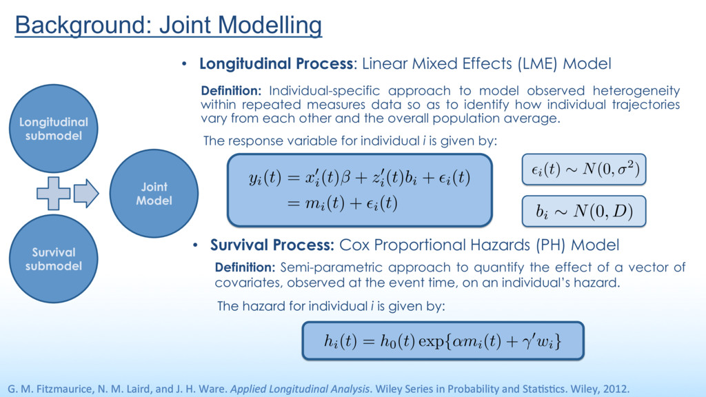
approach to model observed heterogeneity within repeated measures data so as to identify how individual trajectories vary from each other and the overall population average. The response variable for individual i is given by: Longitudinal submodel Survival submodel Joint Model G. M. Fitzmaurice, N. M. Laird, and J. H. Ware. Applied Longitudinal Analysis. Wiley Series in Probability and Sta>s>cs. Wiley, 2012. • Survival Process: Cox Proportional Hazards (PH) Model Definition: Semi-parametric approach to quantify the effect of a vector of covariates, observed at the event time, on an individual’s hazard. The hazard for individual i is given by: yi( t ) = x 0 i ( t ) + z 0 i ( t ) bi + ✏i( t ) = mi( t ) + ✏i( t ) bi ⇠ N(0, D) hi( t ) = h0( t ) exp {↵mi( t ) + 0wi } ✏i(t) ⇠ N(0, 2) Background: Joint Modelling
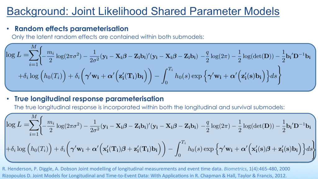
+ ↵0⇣z0 i( Ti) bi ⌘◆ Z Ti 0 h0( s ) exp n 0wi + ↵0⇣z0 i( s ) bi ⌘ods • Random effects parameterisation • True longitudinal response parameterisation Rizopoulos D. Joint Models for Longitudinal and Time-‐to-‐Event Data: With Applica>ons in R. Chapman & Hall, Taylor & Francis, 2012. Background: Joint Likelihood Shared Parameter Models log L = mi 2 log(2 ⇡ 2 ) 1 2 2 ( yi Xi Zibi) 0 ( yi Xi Zibi) q 2 log(2 ⇡ ) 1 2 log(det( D )) 1 2 bi 0D 1bi M X i=1 ( ) log L = mi 2 log(2 ⇡ 2 ) 1 2 2 ( yi Xi Zibi) 0 ( yi Xi Zibi) q 2 log(2 ⇡ ) 1 2 log(det( D )) 1 2 bi 0D 1bi M X i=1 ( Only the latent random effects are contained within both submodels: The true longitudinal response is incorporated within both the longitudinal and survival submodels: R. Henderson, P. Diggle, A. Dobson Joint modelling of longitudinal measurements and event >me data. Biometrics, 1(4):465-‐480, 2000 ) + i log ⇣h0( Ti) ⌘ + i ✓ 0 wi + ↵0⇣ x 0 i(Ti) + z 0 i(Ti)bi ⌘◆ Z Ti 0 h0( s ) exp n 0 wi + ↵0⇣ x 0 i(s) + z 0 i(s)bi ⌘ods
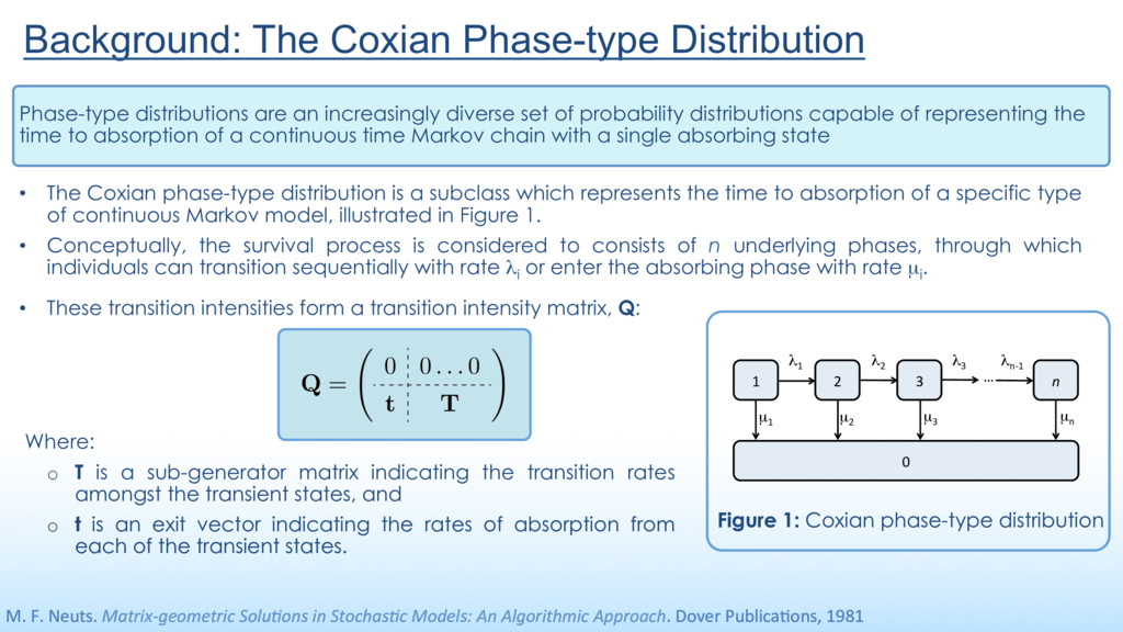
the time to absorption of a specific type of continuous Markov model, illustrated in Figure 1. • Conceptually, the survival process is considered to consists of n underlying phases, through which individuals can transition sequentially with rate λi or enter the absorbing phase with rate µi . • These transition intensities form a transition intensity matrix, Q: Phase-type distributions are an increasingly diverse set of probability distributions capable of representing the time to absorption of a continuous time Markov chain with a single absorbing state M. F. Neuts. Matrix-‐geometric Solu9ons in Stochas9c Models: An Algorithmic Approach. Dover Publica>ons, 1981 1 Background: The Coxian Phase-type Distribution Figure 1: Coxian phase-type distribution 2 3 0 n … λ1 λ2 λ3 λn-‐1 µ1 µ2 µ3 µn Where: o T is a sub-generator matrix indicating the transition rates amongst the transient states, and o t is an exit vector indicating the rates of absorption from each of the transient states.
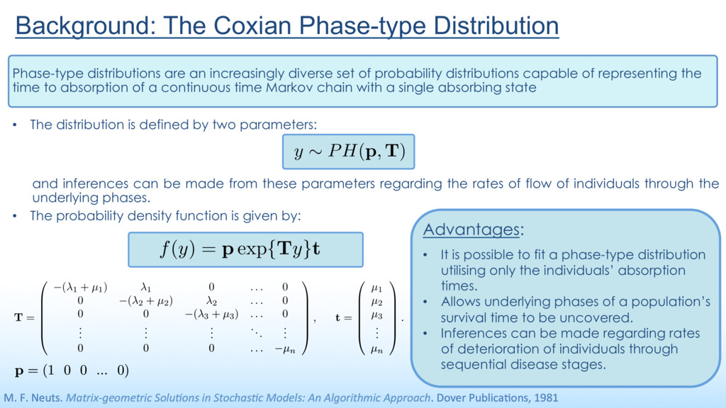
are an increasingly diverse set of probability distributions capable of representing the time to absorption of a continuous time Markov chain with a single absorbing state M. F. Neuts. Matrix-‐geometric Solu9ons in Stochas9c Models: An Algorithmic Approach. Dover Publica>ons, 1981 Background: The Coxian Phase-type Distribution f ( y ) = p exp {Ty}t T = 0 B B B B B @ ( 1 + µ1) 1 0 . . . 0 0 ( 2 + µ2) 2 . . . 0 0 0 ( 3 + µ3) . . . 0 . . . . . . . . . ... . . . 0 0 0 . . . µn 1 C C C C C A , t = 0 B B B B B @ µ1 µ2 µ3 . . . µn 1 C C C C C A . = 0 B B B B B @ ( 1 + µ1) 1 0 . . . 0 0 ( 2 + µ2) 2 . . . 0 0 0 ( 3 + µ3) . . . 0 . . . . . . . . . ... . . . 0 0 0 . . . µn 1 C C C C C A , t = 0 B B B B B @ µ1 µ2 µ3 . . . µn 1 C C C C C A . Advantages: • It is possible to fit a phase-type distribution utilising only the individuals’ absorption times. • Allows underlying phases of a population’s survival time to be uncovered. • Inferences can be made regarding rates of deterioration of individuals through sequential disease stages. • The probability density function is given by: y ⇠ PH(p, T) and inferences can be made from these parameters regarding the rates of flow of individuals through the underlying phases. p = (1 0 0 ... 0)
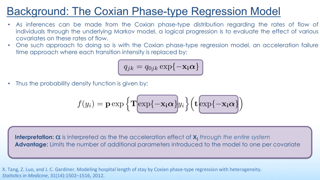
xi through the entire system Advantage: Limits the number of additional parameters introduced to the model to one per covariate X. Tang, Z. Luo, and J. C. Gardiner. Modeling hospital length of stay by Coxian phase-‐type regression with heterogeneity. Sta9s9cs in Medicine, 31(14):1502–1516, 2012. • As inferences can be made from the Coxian phase-type distribution regarding the rates of flow of individuals through the underlying Markov model, a logical progression is to evaluate the effect of various covariates on these rates of flow. • One such approach to doing so is with the Coxian phase-type regression model, an acceleration failure time approach where each transition intensity is replaced by: qjk = q0jk exp { xi↵} f ( yi) = p exp n T exp { xi↵}yi o⇣ t exp { xi↵}⌘ • Thus the probability density function is given by: Background: The Coxian Phase-type Regression Model
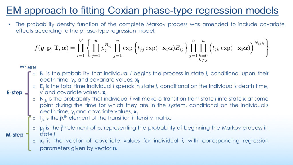
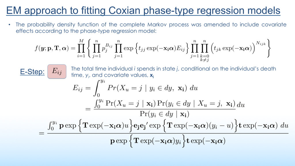
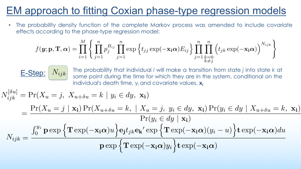
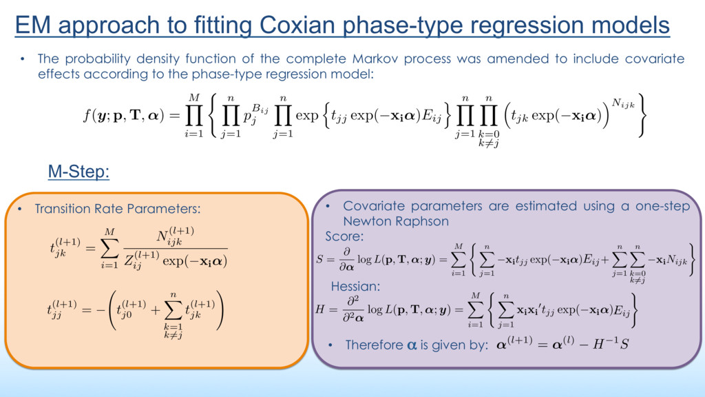
probability density function of the complete Markov process was amended to include covariate effects according to the phase-type regression model: Where o Bij is the probability that individual i begins the process in state j, conditional upon their death time, yi , and covariate values, xi o Eij is the total time individual i spends in state j, conditional on the individual's death time, yi and covariate values, xi o Nijk is the probability that individual i will make a transition from state j into state k at some point during the time for which they are in the system, conditional on the individual's death time, yi and covariate values, xi o tjk is the jkth element of the transition intensity matrix, o pj is the jth element of p, representing the probability of beginning the Markov process in state j o xi is the vector of covariate values for individual i, with corresponding regression parameters given by vector α E-step M-step f ( y ; p , T , ↵ ) = M Y i=1 ( n Y j=1 pBij j n Y j=1 exp ntjj exp( xi↵ ) Eij o n Y j=1 n Y k=0 k6=j ⇣tjk exp( xi↵ ) ⌘Nijk )
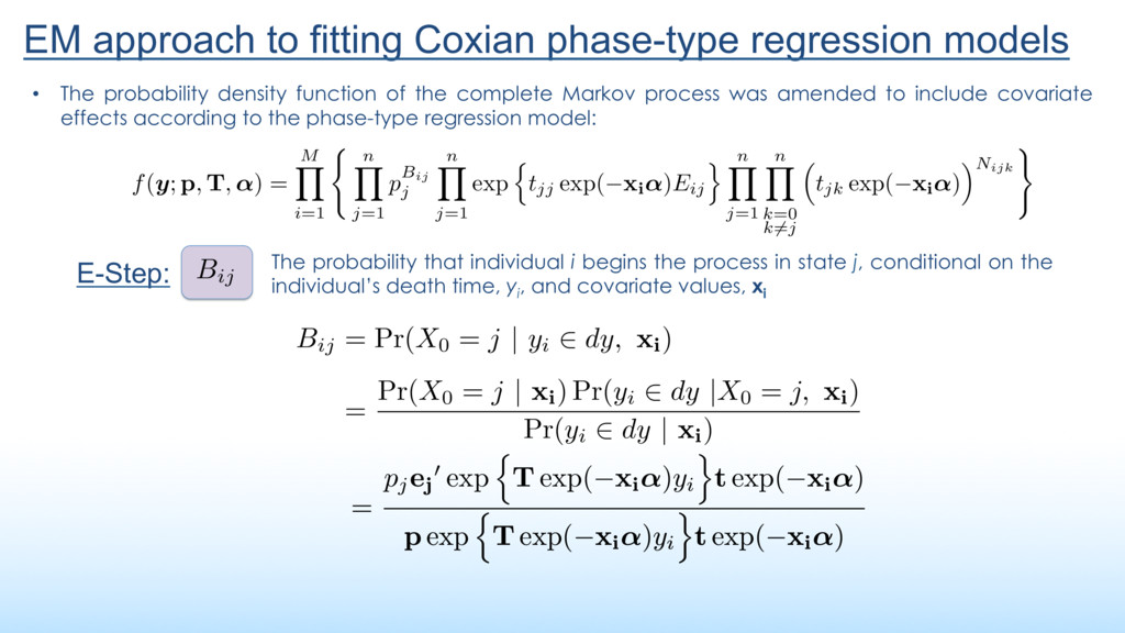
state j, conditional on the individual’s death time, yi , and covariate values, xi Bij = Pr(X0 = j | yi 2 dy, xi) = Pr(X0 = j, yi 2 dy | xi) Pr(yi 2 dy | xi) = Pr(X0 = j | xi) Pr(yi 2 dy |X0 = j, xi) Pr(yi 2 dy | xi) E-Step: Bij = Pr(X0 = j | yi 2 dy, xi) = Pr(X0 = j, yi 2 dy | xi) Pr(yi 2 dy | xi) = Pr(X0 = j | xi) Pr(yi 2 dy |X0 = j, xi) Pr(yi 2 dy | xi) E ⇥B(l+1) ij | yi, xi ⇤ = pjej 0 exp n T exp( xi↵ ) yi o t exp( xi↵ ) p exp n T exp( xi↵ ) yi o t exp( xi↵ ) EM approach to fitting Coxian phase-type regression models • The probability density function of the complete Markov process was amended to include covariate effects according to the phase-type regression model: f ( y ; p , T , ↵ ) = M Y i=1 ( n Y j=1 pBij j n Y j=1 exp ntjj exp( xi↵ ) Eij o n Y j=1 n Y k=0 k6=j ⇣tjk exp( xi↵ ) ⌘Nijk )
conditional on the individual’s death time, yi , and covariate values, xi Zij = Z yi 0 Pr(Xu = j | yi 2 dy, xi) du = R yi 0 Pr(Xu = j | xi) Pr(yi 2 dy | Xu = j, xi) Pr(yi 2 dy | xi) E-Step: = R yi 0 p exp n T exp( xi↵ ) uo ejej 0 exp n T exp( xi↵ )( yi u ) o t exp( xi↵ ) du p exp n T exp( xi↵ ) yi o t exp( xi↵ ) Zij = Z yi 0 Pr(Xu = j | yi 2 dy, xi) du = R yi 0 Pr(Xu = j | xi) Pr(yi 2 dy | Xu = j, xi) Pr(yi 2 dy | xi) = R yi 0 p exp n T exp( xi↵ ) uo ejej 0 exp n T exp( xi↵ )( yi u ) o t exp( xi↵ ) du p exp n T exp( xi↵ ) yi o t exp( xi↵ ) EM approach to fitting Coxian phase-type regression models • The probability density function of the complete Markov process was amended to include covariate effects according to the phase-type regression model: f ( y ; p , T , ↵ ) = M Y i=1 ( n Y j=1 pBij j n Y j=1 exp ntjj exp( xi↵ ) Eij o n Y j=1 n Y k=0 k6=j ⇣tjk exp( xi↵ ) ⌘Nijk ) Eij
state j into state k at some point during the time for which they are in the system, conditional on the individual's death time, yi and covariate values, xi Nijk E-Step: N[ u] ijk = Pr(Xu = j, Xu+ u = k | yi 2 dy, xi) = Pr(Xu = j, Xu+ u = k, yi 2 dy | xi) Pr(yi 2 dy | xi) = Pr(Xu = j | xi) Pr(Xu+ u = k, | Xu = j, yi 2 dy, xi) Pr(yi 2 dy | Xu+ u = k, xi) Pr(yi 2 dy | xi) N[ u] ijk = Pr(Xu = j, Xu+ u = k | yi 2 dy, xi) = Pr(Xu = j, Xu+ u = k, yi 2 dy | xi) Pr(yi 2 dy | xi) = Pr(Xu = j | xi) Pr(Xu+ u = k, | Xu = j, yi 2 dy, xi) Pr(yi 2 dy | Xu+ u = k, xi) Pr(yi 2 dy | xi) = R yi 0 p exp n T exp( xi↵ ) uo ejtjkek 0 exp n T exp( xi↵ )( yi u ) o t exp( xi↵ ) du p exp n T exp( xi↵ ) yi o t exp( xi↵ ) Nijk EM approach to fitting Coxian phase-type regression models • The probability density function of the complete Markov process was amended to include covariate effects according to the phase-type regression model: f ( y ; p , T , ↵ ) = M Y i=1 ( n Y j=1 pBij j n Y j=1 exp ntjj exp( xi↵ ) Eij o n Y j=1 n Y k=0 k6=j ⇣tjk exp( xi↵ ) ⌘Nijk )
= 1 , ..., n and k = 0 , ..., n t(l+1) jj = t(l+1) j0 + n X k=1 k6=j t(l+1) jk ! ↵(l+1) = ↵(l) H 1S • Transition Rate Parameters: • Covariate parameters are estimated using a one-step Newton Raphson Score: H = @2 @2↵ log L (p , T , ↵ ; y ) = M X i=1 ( n X j=1 xixi 0tjj exp( xi↵ ) Zij ) S = @ @↵ log L (p , T , ↵ ; y ) = M X i=1 ( n X j=1 xitjj exp( xi↵ ) Zij + n X j=1 n X k=0 k6=j xiNijk ) Hessian: • Therefore α is given by: EM approach to fitting Coxian phase-type regression models • The probability density function of the complete Markov process was amended to include covariate effects according to the phase-type regression model: t(l+1) jk = M X i=1 N(l+1) ijk Z(l+1) ij exp( xi↵ ) M-Step: f ( y ; p , T , ↵ ) = M Y i=1 ( n Y j=1 pBij j n Y j=1 exp ntjj exp( xi↵ ) Eij o n Y j=1 n Y k=0 k6=j ⇣tjk exp( xi↵ ) ⌘Nijk ) H = @2 @2↵ log L (p , T , ↵ ; y ) = M X i=1 ( n X j=1 xixi 0tjj exp( xi↵ ) Zij ) Eij S = @ @↵ log L (p , T , ↵ ; y ) = M X i=1 ( n X j=1 xitjj exp( xi↵ ) Zij + n X j=1 n X k=0 k6=j xiNijk ) Eij
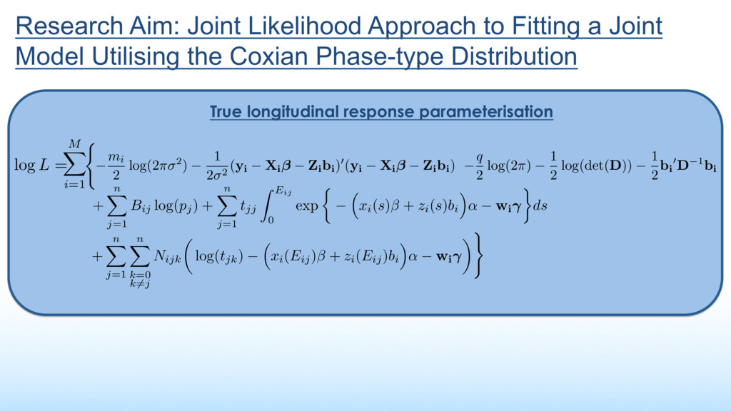
Utilising the Coxian Phase-type Distribution mi 2 log(2 ⇡ 2 ) 1 2 2 ( yi Xi Zibi) 0 ( yi Xi Zibi) q 2 log(2 ⇡ ) 1 2 log(det( D )) 1 2 bi 0D 1bi + n X j=1 Bij log(pj) + n X j=1 tjj Z Eij 0 exp ⇢ ⇣ xi(s) + zi(s)bi ⌘ ↵ wi ds log L = + n X j=1 n X k=0 k6=j Nijk ✓ log(tjk) ⇣ xi(Eij) + zi(Eij)bi ⌘ ↵ wi ◆ M X i=1 ( ) True longitudinal response parameterisation
an individual’s kidney function gradually deteriorates over time, culminating in renal failure and death. The kidneys are responsible for filtering waste products from the body’s blood. • It is commonly observed that anaemia, a condition where the body has a reduced volume of red blood cells, occurs concurrently with CKD patients and that both conditions deteriorate with a similar rate. • Longitudinal biomarker of interest: o Haemoglobin (Hb): a protein found in red blood cells whose volume often decreases as CKD progresses. Aim: To model the repeated measures trajectories of individuals’ Hb levels over time and to incorporate some feature of this trajectory within the Coxian phase-type regression model so as to evaluate its affect on the rates of deterioration of individuals through the underlying phases of the disease. Application to Chronic Kidney Disease
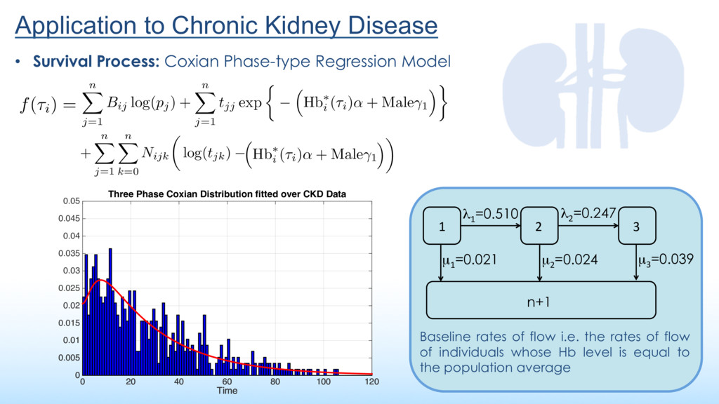
3 µ1 =0.021 µ2 =0.024 λ1 =0.510 λ2 =0.247 µ3 =0.039 • Survival Process: Coxian Phase-type Regression Model n X j=1 Bij log(pj ) + n X j=1 tjj exp ⇢ ⇣ Hb⇤ i (⌧i )↵ + Male 1 + Age 2 ⌘ + n X j=1 n X k=0 Nijk ✓ log(tjk ) ⇣ Hbi (⌧i )↵ + Male 1 + Age 2 ⌘◆ n X j=1 Bij log(pj ) + n X j=1 tjj exp ⇢ ⇣ Hb⇤ i (⌧i )↵ + Male 1 + Age 2 ⌘ + n X j=1 n X k=0 Nijk ✓ log(tjk ) ⇣ Hbi (⌧i )↵ + Male 1 + Age 2 ⌘◆ n X j=1 Bij log(pj ) + n X j=1 tjj exp ⇢ ⇣ Hb⇤ i (⌧i )↵ + Male 1 + Age 2 ⌘ f(⌧i) = Time 0 20 40 60 80 100 120 0 0.005 0.01 0.015 0.02 0.025 0.03 0.035 0.04 0.045 0.05 Three Phase Coxian Distribution fitted over CKD Data Baseline rates of flow i.e. the rates of flow of individuals whose Hb level is equal to the population average
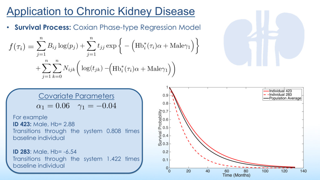
Regression Model n X j=1 Bij log(pj ) + n X j=1 tjj exp ⇢ ⇣ Hb⇤ i (⌧i )↵ + Male 1 + Age 2 ⌘ + n X j=1 n X k=0 Nijk ✓ log(tjk ) ⇣ Hbi (⌧i )↵ + Male 1 + Age 2 ⌘◆ n X j=1 Bij log(pj ) + n X j=1 tjj exp ⇢ ⇣ Hb⇤ i (⌧i )↵ + Male 1 + Age 2 ⌘ + n X j=1 n X k=0 Nijk ✓ log(tjk ) ⇣ Hbi (⌧i )↵ + Male 1 + Age 2 ⌘◆ n X j=1 Bij log(pj ) + n X j=1 tjj exp ⇢ ⇣ Hb⇤ i (⌧i )↵ + Male 1 + Age 2 ⌘ f(⌧i) = Covariate Parameters ↵1 = 0.06 1 = 0.04 For example ID 423: Male, Hb= 2.88 Transitions through the system 0.808 times baseline individual ID 283: Male, Hb= -6.54 Transitions through the system 1.422 times baseline individual Time (Months) 0 20 40 60 80 100 120 140 Survival Probability 0 0.1 0.2 0.3 0.4 0.5 0.6 0.7 0.8 0.9 1 Individual 423 Individual 283 Population Average
![Thank You For Listening Any questions? ? [email protected]](https://files.speakerdeck.com/presentations/a3b5381a1ed0486ab029af081a52fed3/slide_16.jpg)