David Hughes

Transcript

1. Dynamic Longitudinal Discriminant Analysis: Statistical and clinical findings from The DiALog project D. Hughes Introduction Longitudinal Discriminant analysis Credible Intervals Statistical Findings Clinical Findings Dynamic Longitudinal Discriminant Analysis: Statistical and clinical findings from The DiALog project David Hughes 2017
2. Clinical Scenario Time since diagnosis Baseline Data • Age • Sex • Disease Duration • Disease Type • Ethnicity • EEG results • … Follow-up 1 • Blood Tests • Imaging • Questionnaire • … Follow-up 2 • Blood Tests • Imaging • Questionnaire • … Follow-up … • Blood Tests • Imaging • Questionnaire • … OUTCOME • Does patient have the disease or not?
3. Dynamic Longitudinal Discriminant Analysis: Statistical and clinical findings from The DiALog project D. Hughes Introduction Longitudinal Discriminant analysis Credible Intervals Statistical Findings Clinical Findings Some questions... ◮ How can we use changes in longitudinal markers over time to make decisions on clinical outcomes? (eg. Does a patient have drug resistant epilepsy?) ◮ How can we model correlation between repeated measures of multiple markers. ◮ Are predictions equally sure for all patients?
4. Dynamic Longitudinal Discriminant Analysis: Statistical and clinical findings from The DiALog project D. Hughes Introduction Longitudinal Discriminant analysis Credible Intervals Statistical Findings Clinical Findings Longitudinal discriminant analysis (LoDA) ◮ Discriminant analysis models changes in different groups of patients (whose status is known) separately ◮ Predictions of group membership are made to assess which group a new patient is most similar to. ◮ In LoDA, these predictions are calculated using a patient’s longitudinal history.
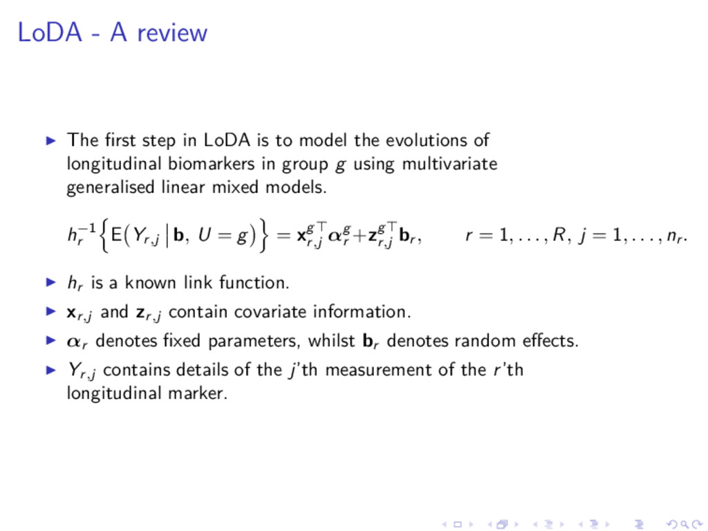
5. LoDA - A review ◮ The first step in LoDA is to model the evolutions of longitudinal biomarkers in group g using multivariate generalised linear mixed models. h−1 r E Yr , j b, U = g = xg⊤ r , j αg r +zg⊤ r , j br , r = 1, . . . , R, j = 1, . . . , nr . ◮ hr is a known link function. ◮ xr , j and zr , j contain covariate information. ◮ αr denotes fixed parameters, whilst br denotes random effects. ◮ Yr , j contains details of the j’th measurement of the r’th longitudinal marker.
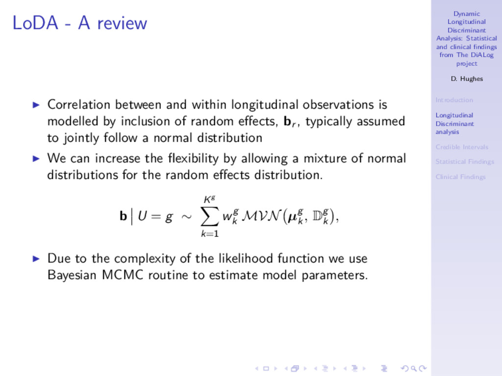
6. Dynamic Longitudinal Discriminant Analysis: Statistical and clinical findings from The DiALog project D. Hughes Introduction Longitudinal Discriminant analysis Credible Intervals Statistical Findings Clinical Findings LoDA - A review ◮ Correlation between and within longitudinal observations is modelled by inclusion of random effects, br , typically assumed to jointly follow a normal distribution ◮ We can increase the flexibility by allowing a mixture of normal distributions for the random effects distribution. b U = g ∼ Kg k=1 wg k MVN µg k , Dg k , ◮ Due to the complexity of the likelihood function we use Bayesian MCMC routine to estimate model parameters.
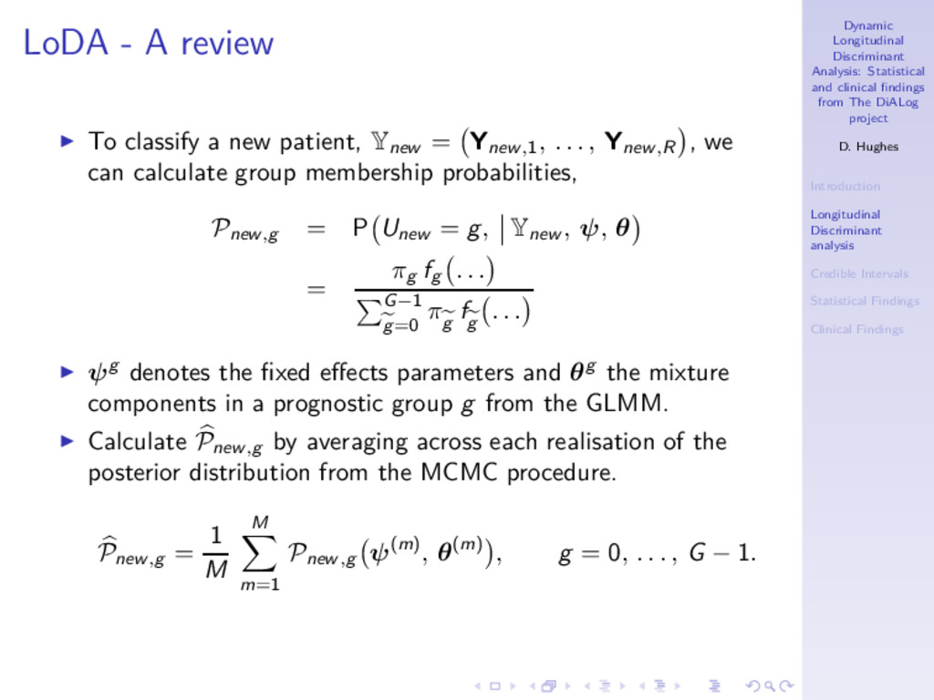
7. Dynamic Longitudinal Discriminant Analysis: Statistical and clinical findings from The DiALog project D. Hughes Introduction Longitudinal Discriminant analysis Credible Intervals Statistical Findings Clinical Findings LoDA - A review ◮ To classify a new patient, Ynew = Ynew , 1, . . . , Ynew , R , we can calculate group membership probabilities, Pnew , g = P Unew = g, Ynew , ψ, θ = πg fg . . . G−1 g=0 πg f g . . . ◮ ψg denotes the fixed effects parameters and θg the mixture components in a prognostic group g from the GLMM. ◮ Calculate Pnew , g by averaging across each realisation of the posterior distribution from the MCMC procedure. Pnew , g = 1 M M m=1 Pnew , g ψ(m) , θ(m) , g = 0, . . . , G − 1.
8. 3 ways to choose the predictive density ◮ Marginal Prediction f marg g y1, . . . , yR ; ψg , θg = f cond g y1, . . . , yR b; ψg f ranef g b; θg db, ◮ Conditional Prediction f cond g y1, . . . , yR b; ψg = R r=1 nr j=1 pr yr , j b; ψg , ◮ Random Effects f ranef g b; θg = Kg k=1 wg k ϕ(b; µg k , Dg k ) ◮ ψg denotes the fixed effects parameters and θg the mixture components in a prognostic group g from the GLMM.
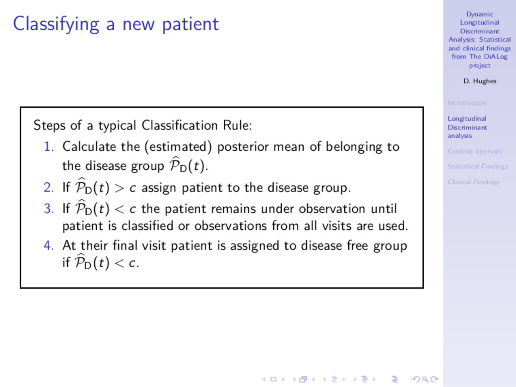
9. Dynamic Longitudinal Discriminant Analysis: Statistical and clinical findings from The DiALog project D. Hughes Introduction Longitudinal Discriminant analysis Credible Intervals Statistical Findings Clinical Findings Classifying a new patient Steps of a typical Classification Rule: 1. Calculate the (estimated) posterior mean of belonging to the disease group PD (t). 2. If PD (t) > c assign patient to the disease group. 3. If PD (t) < c the patient remains under observation until patient is classified or observations from all visits are used. 4. At their final visit patient is assigned to disease free group if PD (t) < c.
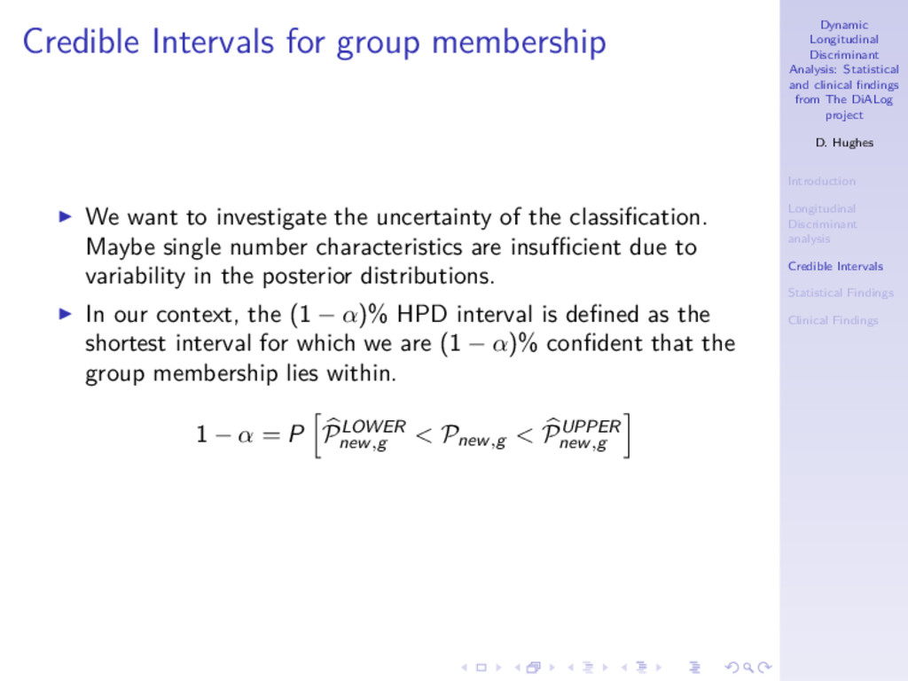
10. Dynamic Longitudinal Discriminant Analysis: Statistical and clinical findings from The DiALog project D. Hughes Introduction Longitudinal Discriminant analysis Credible Intervals Statistical Findings Clinical Findings Credible Intervals for group membership ◮ We want to investigate the uncertainty of the classification. Maybe single number characteristics are insufficient due to variability in the posterior distributions. ◮ In our context, the (1 − α)% HPD interval is defined as the shortest interval for which we are (1 − α)% confident that the group membership lies within. 1 − α = P PLOWER new , g < Pnew , g < PUPPER new , g
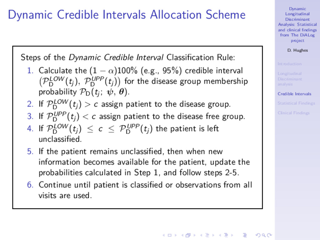
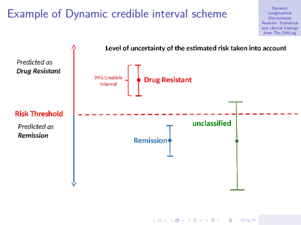
11. Dynamic Longitudinal Discriminant Analysis: Statistical and clinical findings from The DiALog project D. Hughes Introduction Longitudinal Discriminant analysis Credible Intervals Statistical Findings Clinical Findings Dynamic Credible Intervals Allocation Scheme Steps of the Dynamic Credible Interval Classification Rule: 1. Calculate the (1 − α)100% (e.g., 95%) credible interval PLOW D (tj ), PUPP D (tj ) for the disease group membership probability PD (tj ; ψ, θ). 2. If PLOW D (tj ) > c assign patient to the disease group. 3. If PUPP D (tj ) < c assign patient to the disease free group. 4. If PLOW D (tj ) ≤ c ≤ PUPP D (tj ) the patient is left unclassified. 5. If the patient remains unclassified, then when new information becomes available for the patient, update the probabilities calculated in Step 1, and follow steps 2-5. 6. Continue until patient is classified or observations from all visits are used.
12. Dynamic Longitudinal Discriminant Analysis: Statistical and clinical findings from The DiALog project D. Hughes Introduction Longitudinal Discriminant analysis Credible Intervals Statistical Findings Clinical Findings Benefits of using credible intervals ◮ Ideal aim is that false positives and false negatives from the original single number prediction are now left unclassified. ◮ More sure about patients predicted as having disease, so more confident of proposing alternative treatment. ◮ Unclassified patients represent hard to predict ones so we wait longer for these patients to decide on their status. ◮ In some scenarios the unclassified group could represent a group to be sent for more expensive tests to diagnose disease status. Cheap diagnostic tool identifies some patients we are sure about to save using expensive/intrusive tests on all patients.
13. Dynamic Longitudinal Discriminant Analysis: Statistical and clinical findings from The DiALog project D. Hughes Introduction Longitudinal Discriminant analysis Credible Intervals Statistical Findings Clinical Findings Statistical Findings for LoDA ◮ We illustrate some findings using data from the SANAD study. ◮ Main goal is to identify patients with drug resistant epilepsy as soon as possible. ◮ 1577 patients achieved 12-month remission within five years of randomisation, 175 did not (drug resistant!) ◮ Longitudinal variables: Seizures since last visit (Yes/No), total seizures since last vist, number of adverse events ◮ Plus baseline covariates . . . ◮ More details in papers referred to.
14. Dynamic Longitudinal Discriminant Analysis: Statistical and clinical findings from The DiALog project D. Hughes Introduction Longitudinal Discriminant analysis Credible Intervals Statistical Findings Clinical Findings Example of Dynamic credible interval scheme
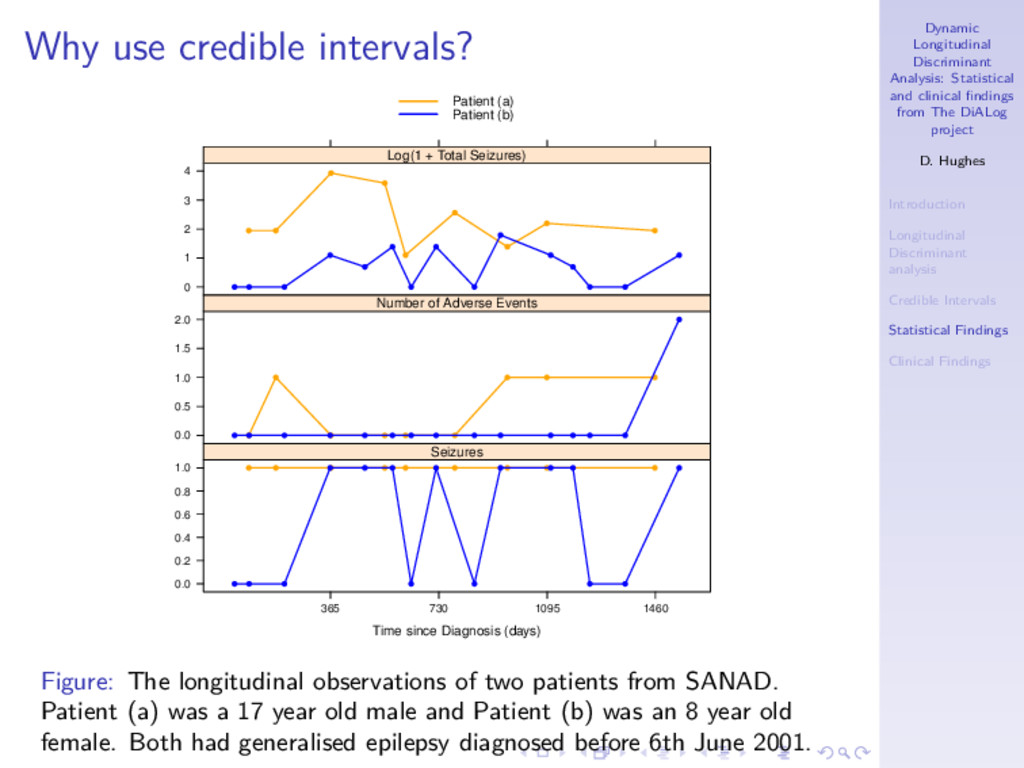
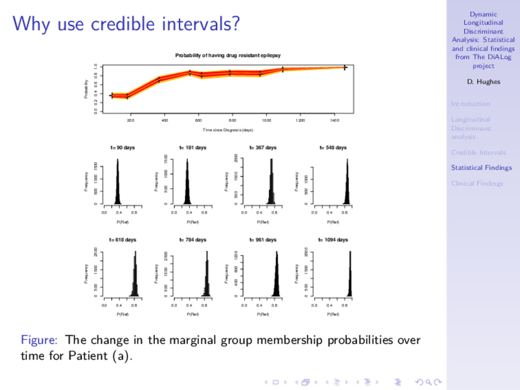
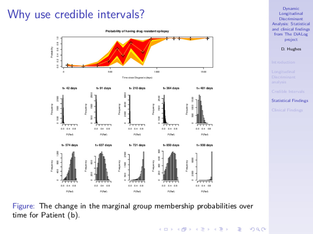
15. Dynamic Longitudinal Discriminant Analysis: Statistical and clinical findings from The DiALog project D. Hughes Introduction Longitudinal Discriminant analysis Credible Intervals Statistical Findings Clinical Findings Why use credible intervals? Time since Diagnosis (days) 0.0 0.2 0.4 0.6 0.8 1.0 365 730 1095 1460 Seizures 0.0 0.5 1.0 1.5 2.0 Number of Adverse Events 0 1 2 3 4 Log(1 + Total Seizures) Patient (a) Patient (b) Figure: The longitudinal observations of two patients from SANAD. Patient (a) was a 17 year old male and Patient (b) was an 8 year old female. Both had generalised epilepsy diagnosed before 6th June 2001.
16. Dynamic Longitudinal Discriminant Analysis: Statistical and clinical findings from The DiALog project D. Hughes Introduction Longitudinal Discriminant analysis Credible Intervals Statistical Findings Clinical Findings Why use credible intervals? + + + + + + + + + 200 400 600 800 1000 1200 1400 0.0 0.2 0.4 0.6 0.8 1.0 Probability of having drug resistant epilepsy Time since Diagnosis (days) Probability + + + + + + + + + t= 90 days P(Ref) Frequency 0.0 0.4 0.8 0 500 1000 1500 t= 181 days P(Ref) Frequency 0.0 0.4 0.8 0 500 1000 1500 t= 367 days P(Ref) Frequency 0.0 0.4 0.8 0 500 1500 2500 t= 548 days P(Ref) Frequency 0.0 0.4 0.8 0 500 1000 t= 618 days P(Ref) Frequency 0.0 0.4 0.8 0 500 1500 2500 t= 784 days P(Ref) Frequency 0.0 0.4 0.8 0 500 1500 2500 t= 961 days P(Ref) Frequency 0.0 0.4 0.8 0 400 800 1200 t= 1094 days P(Ref) Frequency 0.0 0.4 0.8 0 500 1500 2500 Figure: The change in the marginal group membership probabilities over time for Patient (a).
17. Dynamic Longitudinal Discriminant Analysis: Statistical and clinical findings from The DiALog project D. Hughes Introduction Longitudinal Discriminant analysis Credible Intervals Statistical Findings Clinical Findings Why use credible intervals? ++ + + + + + + + + + + + + + 0 500 1000 1500 0.0 0.2 0.4 0.6 0.8 1.0 Probability of having drug resistant epilepsy Time since Diagnosis (days) Probability ++ + + + + + + + + + + + + + t= 42 days P(Ref) Frequency 0.0 0.4 0.8 0 500 1500 2500 t= 91 days P(Ref) Frequency 0.0 0.4 0.8 0 500 1500 2500 t= 210 days P(Ref) Frequency 0.0 0.4 0.8 0 2000 4000 6000 t= 364 days P(Ref) Frequency 0.0 0.4 0.8 0 500 1500 2500 t= 481 days P(Ref) Frequency 0.0 0.4 0.8 0 500 1000 1500 t= 574 days P(Ref) Frequency 0.0 0.4 0.8 0 400 800 1200 t= 637 days P(Ref) Frequency 0.0 0.4 0.8 0 200 600 t= 721 days P(Ref) Frequency 0.0 0.4 0.8 0 500 1500 2500 t= 850 days P(Ref) Frequency 0.0 0.4 0.8 0 200 400 600 800 t= 938 days P(Ref) Frequency 0.0 0.4 0.8 0 2000 6000 Figure: The change in the marginal group membership probabilities over time for Patient (b).
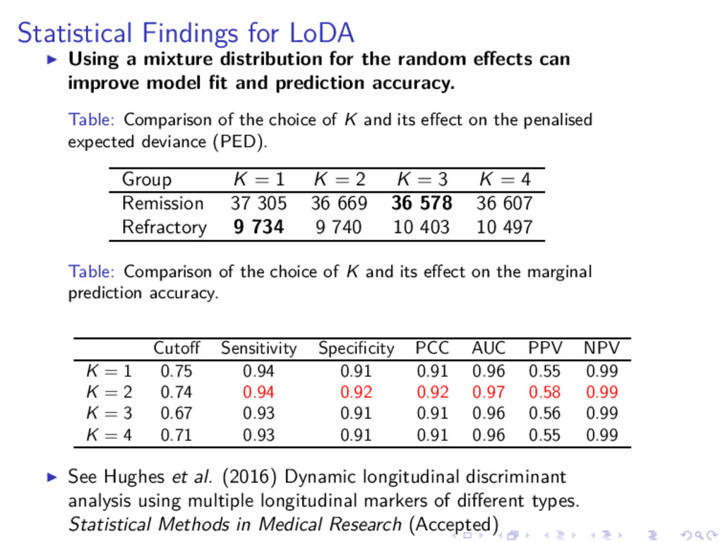
18. Statistical Findings for LoDA ◮ Using a mixture distribution for the random effects can improve model fit and prediction accuracy. Table: Comparison of the choice of K and its effect on the penalised expected deviance (PED). Group K = 1 K = 2 K = 3 K = 4 Remission 37 305 36 669 36 578 36 607 Refractory 9 734 9 740 10 403 10 497 Table: Comparison of the choice of K and its effect on the marginal prediction accuracy. Cutoff Sensitivity Specificity PCC AUC PPV NPV K = 1 0.75 0.94 0.91 0.91 0.96 0.55 0.99 K = 2 0.74 0.94 0.92 0.92 0.97 0.58 0.99 K = 3 0.67 0.93 0.91 0.91 0.96 0.56 0.99 K = 4 0.71 0.93 0.91 0.91 0.96 0.55 0.99 ◮ See Hughes et al. (2016) Dynamic longitudinal discriminant analysis using multiple longitudinal markers of different types. Statistical Methods in Medical Research (Accepted)
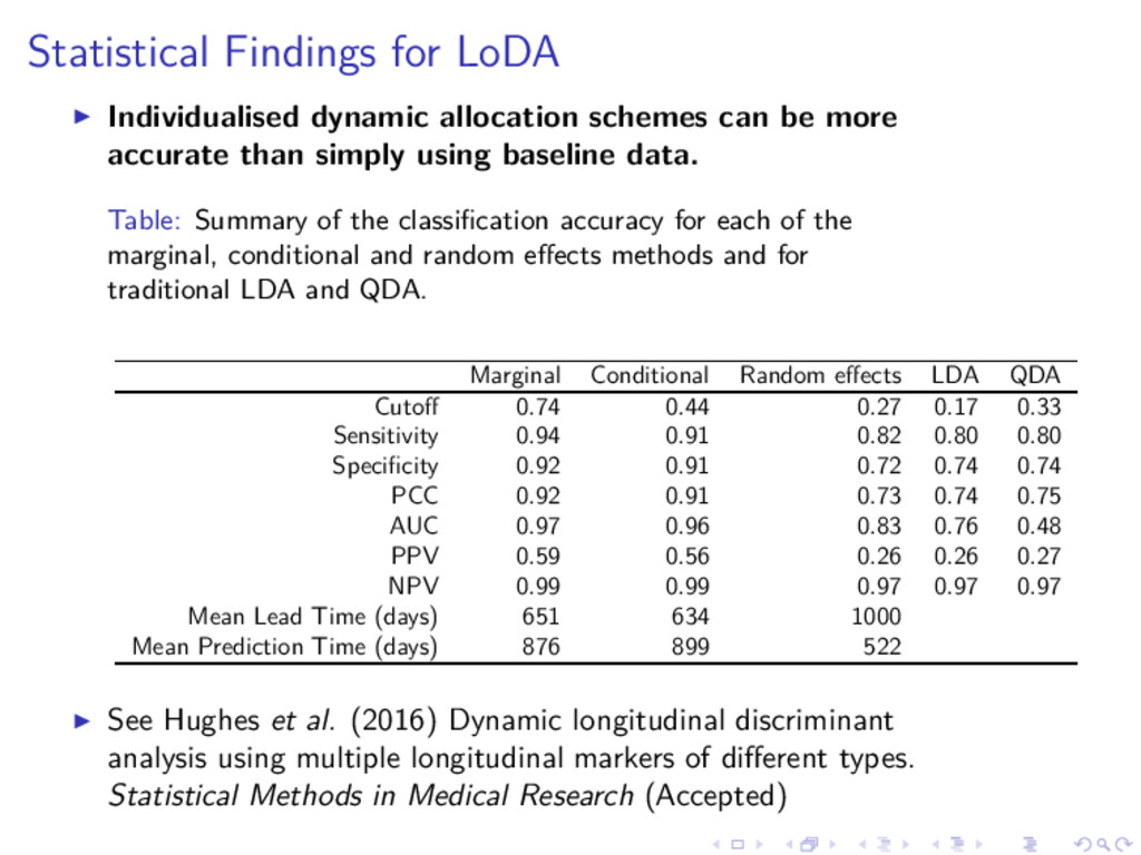
19. Statistical Findings for LoDA ◮ Individualised dynamic allocation schemes can be more accurate than simply using baseline data. Table: Summary of the classification accuracy for each of the marginal, conditional and random effects methods and for traditional LDA and QDA. Marginal Conditional Random effects LDA QDA Cutoff 0.74 0.44 0.27 0.17 0.33 Sensitivity 0.94 0.91 0.82 0.80 0.80 Specificity 0.92 0.91 0.72 0.74 0.74 PCC 0.92 0.91 0.73 0.74 0.75 AUC 0.97 0.96 0.83 0.76 0.48 PPV 0.59 0.56 0.26 0.26 0.27 NPV 0.99 0.99 0.97 0.97 0.97 Mean Lead Time (days) 651 634 1000 Mean Prediction Time (days) 876 899 522 ◮ See Hughes et al. (2016) Dynamic longitudinal discriminant analysis using multiple longitudinal markers of different types. Statistical Methods in Medical Research (Accepted)
20. Statistical Findings for LoDA ◮ Using a credible interval scheme can reduce the number of false positives (increasing PPV). Table: A comparison of the prediction accuracy using dynLoDA and dynCI schemes. The sensitivities and specificities highlighted in bold are calculated without considering the unclassified patients. dynLoDA dynCI dynCI dynCI dynCI 99% HPDCI 95% HPDCI 90% HPDCI 50% HPDCI Cutoff 0.83 0.83 0.83 0.83 0.83 Sensitivity (Classified Data) 0.93 0.95 0.95 0.94 0.93 Sensitivity 0.93 0.86 0.89 0.89 0.93 Specificity (Classified Data) 0.92 0.95 0.94 0.93 0.91 Specificity 0.92 0.91 0.91 0.91 0.90 PCC (Classified Data) 0.92 0.95 0.94 0.93 0.91 PCC 0.92 0.90 0.90 0.90 0.90 AUC 0.97 0.98 0.98 0.97 0.97 PPV 0.56 0.69 0.63 0.61 0.55 NPV 0.99 0.99 0.99 0.99 0.99 Proportion Unclassified 0.00 0.05 0.04 0.03 0.01 Mean Lead Time (days) 675 565 595 614 661 Mean Prediction Time (days) 857 972 942 918 872 ◮ See Hughes et al. (2017) Dynamic classification using credible intervals in longitudinal discriminant analysis Statistics in Medicine (Accepted)
21. Dynamic Longitudinal Discriminant Analysis: Statistical and clinical findings from The DiALog project D. Hughes Introduction Longitudinal Discriminant analysis Credible Intervals Statistical Findings Clinical Findings Statistical Findings for LoDA ◮ The conditional prediction approach offers little benefit over the marginal or random effects prediction methods. ◮ The random effects approach doesn’t work well when the measurement error is thought to be larger than the variation between individuals. ◮ Hughes, El Saeti & Garc´ ıa-Fi˜ nana (2017), A comparison of group prediction approaches in longitudinal discriminant analysis (Biometrical Journal (Accepted))
22. Externally validated prediction model for drug resistant epilepsy. Table: Summary of the predictive accuracy for SANAD, MESS and NGPSE. Dataset Sensitivity Specificity PCC PPV % Unclassified Mean Prediction Time (days) SANAD 0.95 0.97 0.97 0.76 0.055 1112 MESS 0.91 0.97 0.97 0.34 0.005 1291 NGPSE 0.93 0.98 0.98 0.76 0.010 1301
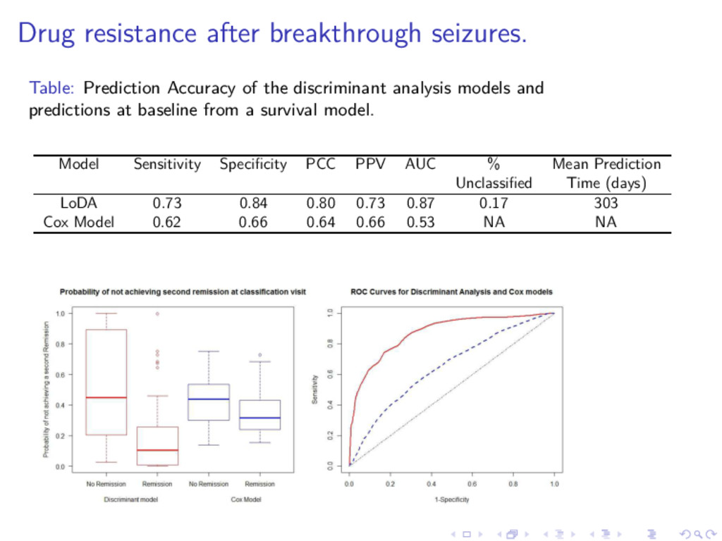
23. Drug resistance after breakthrough seizures. Table: Prediction Accuracy of the discriminant analysis models and predictions at baseline from a survival model. Model Sensitivity Specificity PCC PPV AUC % Mean Prediction Unclassified Time (days) LoDA 0.73 0.84 0.80 0.73 0.87 0.17 303 Cox Model 0.62 0.66 0.64 0.66 0.53 NA NA
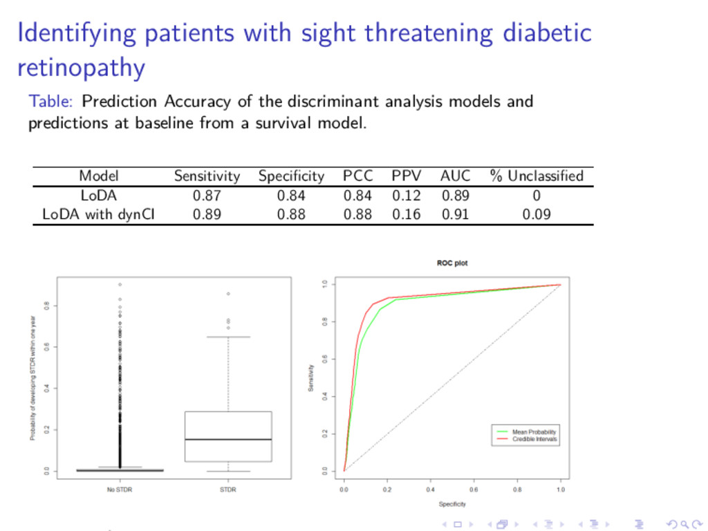
24. Identifying patients with sight threatening diabetic retinopathy Table: Prediction Accuracy of the discriminant analysis models and predictions at baseline from a survival model. Model Sensitivity Specificity PCC PPV AUC % Unclassified LoDA 0.87 0.84 0.84 0.12 0.89 0 LoDA with dynCI 0.89 0.88 0.88 0.16 0.91 0.09
25. Dynamic Longitudinal Discriminant Analysis: Statistical and clinical findings from The DiALog project D. Hughes Introduction Longitudinal Discriminant analysis Credible Intervals Statistical Findings Clinical Findings Acknowledgements ◮ Joint work with Arnoˇ st Kom´ arek (Charles University in Prague), Gabriela Czanner, Laura Bonnett, Tony Marson, Simon Harding, Chris Cheyne and Marta Garc´ ıa-Fi˜ nana. ◮ We acknowledge support from the Medical Research Council (Research project MR/L010909/1). ◮ Garc´ ıa-Fi˜ nana M, Czanner G, Cox T, Bonnett L, Harding S, Marson T. Discriminant Function Analysis for Longitudinal Data: Applications in Medical Research (2014–2017) funded by MRC.