Peter Diggle

Transcript

1. Modelling repeated measurement data with longer-than-Gaussian tails Peter J Diggle combining health information, computation and statistics CHICAS Based on joint work with: Ozgur Asar (Istanbul); David Bolin (Gothenberg); Ines Sousa (Braga); David Taylor-Robinson (Liverpool); Jonas Wallin (Lund)
2. The linear (Gaussian) mixed effects model Yij = x ij β + d ij Ui + Wi (tij ) + Zij Examples Repeated measures ANOVA ??? Random intercept and slope 1982 Random intercept and stationary process 1988
3. An RCT with longitudinal follow-up: schizophrenia 0 2 4 6 8 40 60 80 100 120 140 160 week PANSS
4. An RCT with longitudinal follow-up: schizophrenia 0 2 4 6 8 40 60 80 100 120 140 160 week PANSS
5. An RCT with longitudinal follow-up: schizophrenia 0 2 4 6 8 40 60 80 100 120 140 160 week PANSS
6. RCT results 0 2 4 6 8 70 75 80 85 90 95 100 weeks PANSS haloperidol placebo risperidone
7. Danish cohort study: cystic fibrosis 20:55
8. Danish cohort study: cystic fibrosis 20:48
9. Danish cohort study: cystic fibrosis 20:49
10. CF data: modelling within-subject variation 21 September 2014 20:29
11. CF data: modelling within-subject variation 21 September 2014 20:51
12. CF data: modelling within-subject variation 21 September 2014 20:28
13. A surveillance problem: kidney failure Data from Salford Integrated Records System Number Mean age (SE) all patients 161,781 49.4 (18.6) primary care patients 22,910 65.4 (15.1) irregular time-sequences of eGFR measurements: i = 1, ..., m = 22, 910 primary care patients ni ≤ 654 measurements per patient explanatory variables: age; sex; diabetes; albuminuria
14. Sample log(eGFR) traces 55 60 65 70 75 80 3.0 3.5 4.0 4.5 age (years) log(eGFR)
15. Is the Gaussian assumption critical? For estimating mean response profiles Probably not For predicting individual response profiles Probably For spotting extreme behaviour Almost certainly
16. Extending the Gaussian linear model Yij = x ij β + d ij Ui + Wi (tij ) + Zij any or all of the stochastic terms non-Gaussian continuous-time interpretation for Wi (t) Distributional family Y = µT + √ TΣ1/2Z, µ = E[Y] Σ = var(Y) T ∼ generalized inverse Gaussian distribution (GIG) Z ∼ N(0, I).
17. Non-Gaussian noise Yij = x ij β + d ij Ui + Wi (tij ) + Zij Zij = τ Tij Z∗ ij Tij ∼ iid GIG Z∗ ij ∼ iidN(0, 1).
18. Non-Gaussian random effects Yij = x ij β + d ij Ui + Wi (tij ) + Zij Ui = Ti U∗ i Ti ∼ iid GIG U∗ i ∼ iidN(0, V).
19. Non-Gaussian stochastic process Yij = x ij β + d ij Ui + Wi (tij ) + Zij DWi (t) = dLi (t), D = differential operator dLi ∼ continuous-time white noise (⇒ Wi (t) at least continuous) Integrated random walk: D = ∂2 ∂t2 Matérn: D = ( ∂2 ∂t2 − κ)α/2
20. Low-rank approximation Yij = x ij β + d ij Ui + Wi (tij ) + Zij W(t) = m j=1 φj (t)Wj Wj = Tj W∗ j Tj ∼ iid GIG W∗ j ∼ iidN(0, V) φ1 (t), ..., φm (t) : solution of discretised differential equation
21. Danish CF dataset • Patients seen monthly • 70,448 measures on 497 patients between 1969 and 2010 • Median follow up 10.5 years • 6500 person-years follow-up
22. Analysing the CF cohort data Twin objectives estimate covariate effects individual-level prediction to inform clinical decisions Linear mixed effects model Yij = xij β + Ui + Wi (tij ) + Zij , Gaussian and non-Gaussian variants Ui , Wi (tij ), Zij
23. CF data: empirical variogram and fitted Gaussian model
24. CF data: model simulations and data
25. CF data: residuals vs fitted values
26. CF data: Gaussian model OK? Comparing predictive inferences Distribution Results Process Random Effects Noise MAE Coverage Width None Normal Normal 8.9 94.3 45.2 None GIG GIG 8.6 94.6 45.8 Normal Normal Normal 5.6 94.1 30.0 GIG GIG GIG 5.6 93.9 29.5
27. CF data: mean response parameter estimates Adjusted for age-by-cohort interactions Parameter Estimate 95% CI Intercept at age 5 years 66.02 61.13 70.92 Diabetes -2.47 -3.58 -1.37 Age -0.26 -0.49 -0.03 Pancreatic sufficiency 2.78 -10.43 15.99 Pseudomonas aeruginosa infection -0.51 -0.72 -0.29
28. CF data: prediction for one patient 21 September 2014 20:28
29. Kidney failure: diagnosis, treatment and survival Diagnosis Serum creatinine ⇒ estimated glomerular filtration rate eGFR = 186 × SCr 88.4 −1.154 × age−0.203(×0.742 if female) progression can be asymptomatic for many years SCr easy to measure from blood-sample (but noisy) Treatment and survival aggressive control of blood-pressure renal replacement therapy: dialysis and transplantation early diagnosis and intervention can slow rate of progression Survival rate (%) to year 1 2 5 10 Dialysis 79.3 64.7 33.6 10.2 Transplant (living) 98.4 96.5 90.0 76.0
30. Royal Salford Hospital, NW England Clinical guideline Loss of > 5% eGFR per year ⇒ refer to secondary care Data measurements Yij = log eGFR at times tij , explanatory variables xi (age, sex) i = 1, ..., m = 22, 910 “at-risk” primary care patients j = 1, ..., ni ≤ 305 (median ni = 12) 0 ≤ 10.02 years follow-up (median 4.46) Hi (t) = {xi , (tij , yij ) : tij ≤ t} Statistical objective P d dt log GFR < −0.05|Hi (t) = ?
31. Data: all cross-sectional and selected longitudinal
32. Dynamic regression model subjects i = 1, ..., n observed at times tij , j = 1, ...ni Yij = log(eGFR) expected value of Yij linear in initial age and time since recruitment rate of progression varies randomly: between subjects: random effect Ui within subjects: random effect Ci (tij )
33. Dynamic Regression Model Yij = α0 + α1 × I(female) + β1 × agei1 + β2 × (ageij − agei1 ) + β3 × max(0, ageij − 56.5) + Ui + Ci (tij ) + Zij Zij : measurement error, N(0, τ2) Ui : between-subject random intercept, N(0, ω2) Ci (t): within-subject stochastic process Model Ci (t) as integrated Brownian motion Ci (t) = t 0 Bi (u)du Bi (u)|Bi (s) ∼ N Bi (u), (u − s)σ2 Bi (u) is rate of progression for subject i at time t
34. Maximum likelihood estimates of model parameters RE(%)= 100(exp( ˆ β) − 1) corresponds to estimated annual percentage change in renal function Parameter Estimate SE RE(%) α0 intercept 4.6006 0.0203 α1 female -0.0877 0.0048 -8.4 β1 age on entry -0.0048 0.0004 -0.5 β2 follow-up -0.0232 0.0011 -2.3 β3 age>56.5 -0.0075 0.0006 -0.6 ω2 intercept 0.1111 0.0012 σ2 signal 0.0141 0.0002 τ2 noise 0.0469 0.0001
35. Modelling progression 55 60 65 70 75 80 3.0 3.5 4.0 4.5 age (years) log(eGFR)
36. Modelling progression 55 60 65 70 75 80 3.0 3.5 4.0 4.5 age (years) log(eGFR)
37. Modelling progression 55 60 65 70 75 80 3.0 3.5 4.0 4.5 age (years) log(eGFR) Predicting rate of change in GFR
38. Kidney failure data: Gaussian model OK? Comparing predictive inferences Distribution Results Process Random Effects Noise MAE Coverage Width None Normal Normal 0.175 93.80 1.020 None GIG Normal 0.178 93.86 1.014 None GIG GIG 0.182 92.79 0.971 Normal Normal Normal 0.168 93.82 0.990 Normal Normal GIG 0.126 94.95 0.910 GIG Normal Normal 0.119 96.13 0.794 GIG GIG Normal 0.169 92.37 0.847 GIG GIG GIG 0.115 95.63 0.801
39. Prediction: classic progression pattern q q q q q q q q q q q q q q q qq q q q q q q q 0.0 0.5 1.0 1.5 2.0 2.5 3.0 3.5 Follow−up time (in years) log(eGFR) 0.0 0.5 1.0 1.5 2.0 −0.8 −0.6 −0.4 −0.2 0.0 0.2 Follow−up time (in years) B ~ 0.0 0.5 1.0 1.5 2.0 0.0 0.2 0.4 0.6 0.8 1.0 Follow−up time (in years) Probability
40. Prediction: AKI (Acute Kidney Injury) recovery q q q q q q q q q q q q q q q q q q q q q q q q q q q q q q q q q q q q q q 0 1 2 3 4 5 3.8 4.0 4.2 4.4 4.6 4.8 5.0 Follow−up time (in years) log(eGFR) 0 1 2 3 4 5 −0.4 −0.2 0.0 0.2 0.4 Follow−up time (in years) B ~ 0 1 2 3 4 5 0.0 0.2 0.4 0.6 0.8 1.0 Follow−up time (in years) Probability
41. Prediction: non-recovery from AKI q q q q q q q q q q q q q q q q q q q q q q q q q q q q q q q q q q q q q q q q q q q q q q q q q q q q q q q q q q q q q q q q q q q q q q q q q q q q q q q q q q q q q q 0.0 0.5 1.0 1.5 2.0 2.5 2.5 3.0 3.5 4.0 Follow−up time (in years) log(eGFR) 0.0 0.5 1.0 1.5 2.0 2.5 −1.0 −0.5 0.0 0.5 Follow−up time (in years) B ~ 0.0 0.5 1.0 1.5 2.0 2.5 0.0 0.2 0.4 0.6 0.8 1.0 Follow−up time (in years) Probability
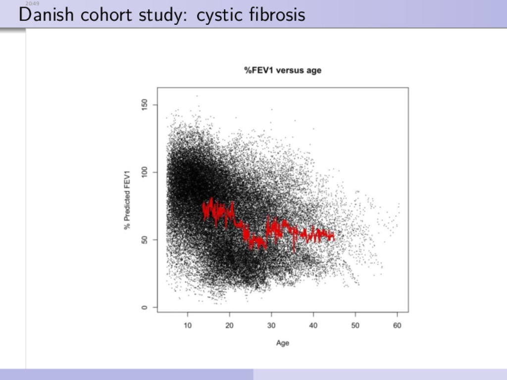
42. References RCT case-study Diggle, P.J. (1998). Dealing with missing values in longitudinal studies. In Recent Advances in the Statistical Analysis of Medical Data, ed. B.S. Everitt and G. Dunn, 203-28. London : Arnold. Cystic fibrosis case-study Taylor-Robinson,D., Whitehead,M., Diderichsen, F., Olesen, H.V., Pressler, T., Smyth, R.L. and Diggle, P. (2012). Understanding the natural progression in %FEV1 decline in patients with cystic fibrosis: a longitudinal study. Thorax, 67, 860–866. doi 10.1136/thoraxjnl-2011-200953 Kidney failure case-study Diggle, P.J., Sousa, I. and Asar, O. (2015). Real-time monitoring of progression towards renal failure in primary care patients. Biostatistics, 16, 522–536 Non-Gaussian modelling Asar, O., Bolin, D., Diggle, P.J. and Wallin, J. (2017). Analysis of non-Gaussian repeated measurement data. In preparation