Gerrit Toenges

Transcript

1. Recurrent event analysis in the presence of an associated terminal event: Bias of marginal model estimates Gerrit Toenges Institute of Medical Biostatistics, Epidemiology and Informatics (IMBEI) University Medical Center Mainz July 4th 2017
2. Motivation: Val-HeFT-trial Valsartan Heart Failure Trial1 (Val-HeFT) Randomised clinical trial on the efficacy of Valsartan in chronic heart failure (HF): Treatment group (n = 2511): Standard therapy + Valsartan Control group (n = 2499) : Standard therapy + Placebo Endpoints: 1. Mortality (time to death) 2. Morbidity (time to recurrent hospitalisations) Pat. 1 Pat. 2 Randomisation End of study = Hospitalisation = Death = Censoring (administrative) 1 Cohn, J.R. et al. (2001): A Randomized Trial of the Angiotensin-Receptor Blocker Valsartan in Chronic Heart Failure. N Engl J Med; 345:1667-1675 2
3. Modelling approaches λ1 (t) = Hospitalisation rate of survivors λ2 (t) = Mortality rate of survivors → Poisson-assumption: Both rates independent of event history 0 H1 H2 H3 ... D D D ... λ1 (t) λ2 (t) λ1 (t) λ2 (t) λ1 (t) λ2 (t) λ1 (t) λ2 (t) time t H = Hosp. D = Death Marginal Models (Conditional independent processes) λ1 (t|x) = λ10 (t) exp(βT 1 x) λ2 (t|x) = λ20 (t) exp(βT 2 x) Joint Frailty Model (Associated processes) λ1 (t|Z, x) = Zλ10 (t) exp(βT 1 x) λ2 (t|Z, x) = Zλ20 (t) exp(βT 2 x) 3
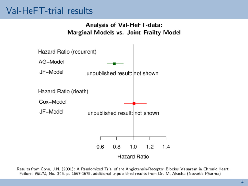
4. Val-HeFT-trial results Analysis of Val-HeFT-data: Marginal Models vs. Joint Frailty Model 0.6 0.8 1.0 1.2 1.4 unpublished result: not shown unpublished result: not shown Hazard Ratio (recurrent) AG−Model JF−Model Hazard Ratio (death) Cox−Model JF−Model Hazard Ratio Results from Cohn, J.N. (2001): A Randomized Trial of the Angiotensin-Receptor Blocker Valsartan in Chronic Heart Failure. NEJM, No. 345, p. 1667-1675, additional unpublished results from Dr. M. Akacha (Novartis Pharma) 4
5. Question: Bias of misspecified marginal model estimates True data-generating model: Joint Frailty Model Hospitalisations : λ1 (t|Z, x) = Zλ10 (t) exp(βT 1 x) Mortality : λ2 (t|Z, x) = Zλ20 (t) exp(βT 2 x) Analysis by misspecified marginal models Hospitalisations : λ1 (t|x) = λ10 (t) exp(βT 1 x) → Andersen-Gill model Mortality : λ2 (t|x) = λ20 (t) exp(βT 2 x) → Cox model Maximum partial likelihood estimation: βAG 1 = argmax β∈Rp n i=1 j:Tij <min{Ci ,Di } exp(βT Xi ) k∈R(Tij ) exp(βT Xk ) 5
6. Marginal properties of the Joint Frailty Model Non-proportional marginal hospitalisation-hazards Gamma-Frailty, exp(β2) = 0.61, exp(β1) = 0.74 λ10(t) = const1, λ20(t) = const2 0.0 0.5 1.0 1.5 2.0 2.0 2.5 3.0 a Marginaler Hazard Control (x=0) Treatment (x=1) 0.0 0.5 1.0 1.5 2.0 a 0.74 0.76 0.78 0.80 time Marginal Hazard Ratio Marginal Hazard Marginal Hazard λ1(t|x) = λ10(t) exp(β1x) E(Z|x, D > t) decreasing in t Marginal Hazard Ratio λ1(t|x = 1) λ1(t|x = 0) = exp(β1) E(Z|x = 1, D > t) E(Z|x = 0, D > t) 6
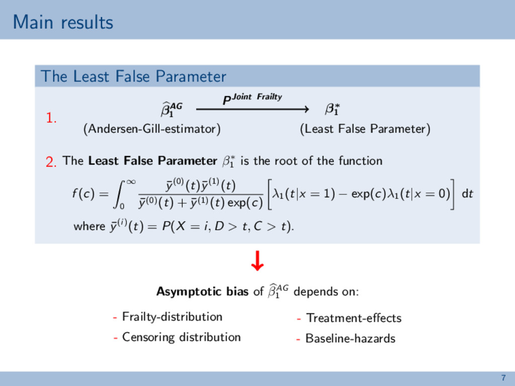
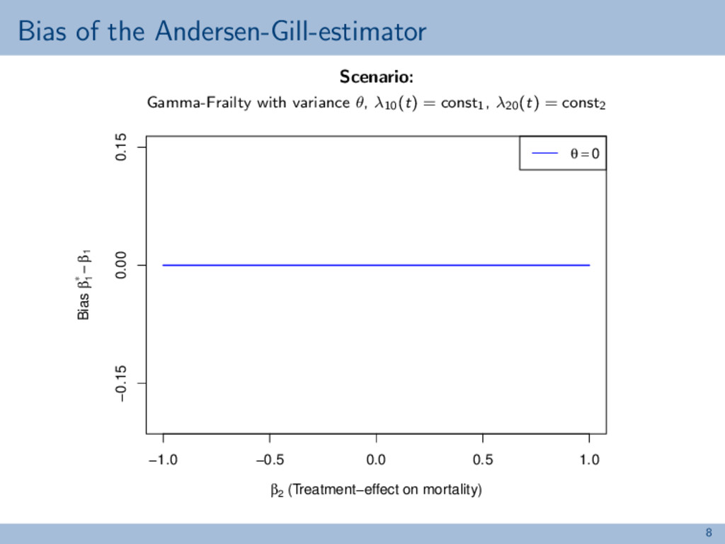
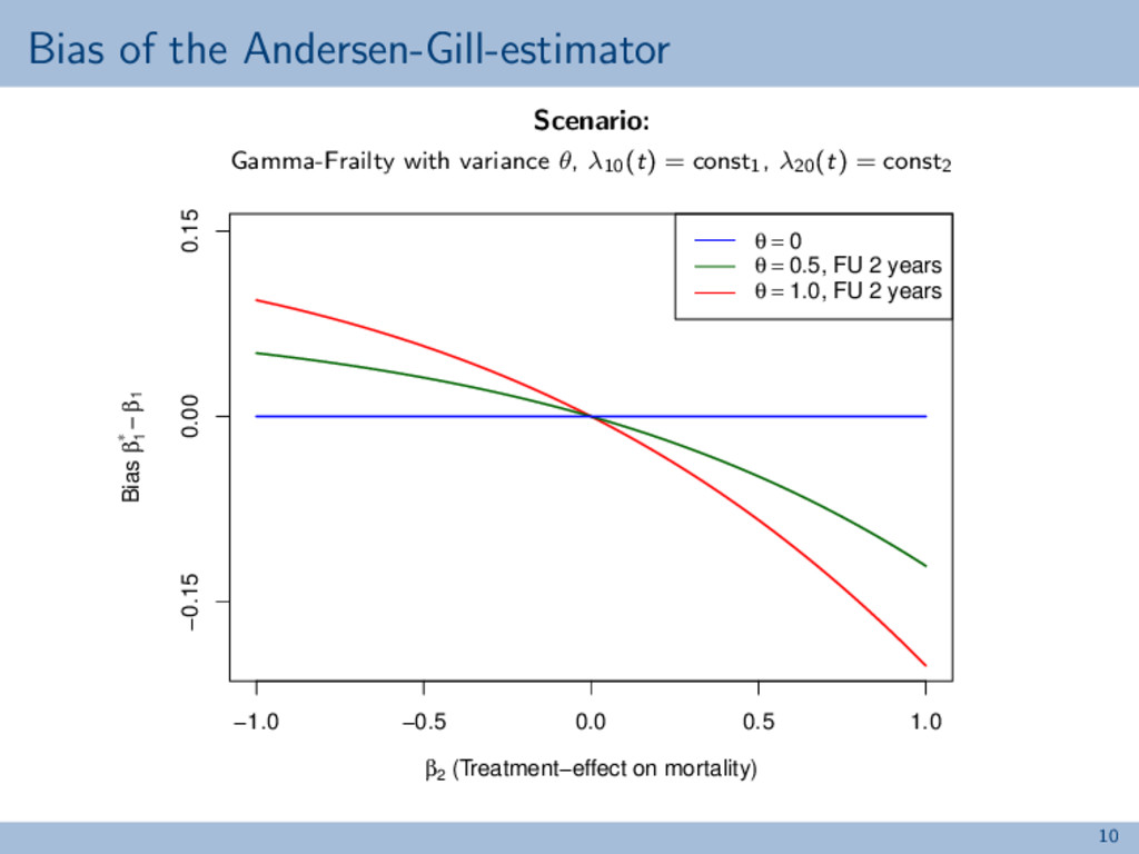
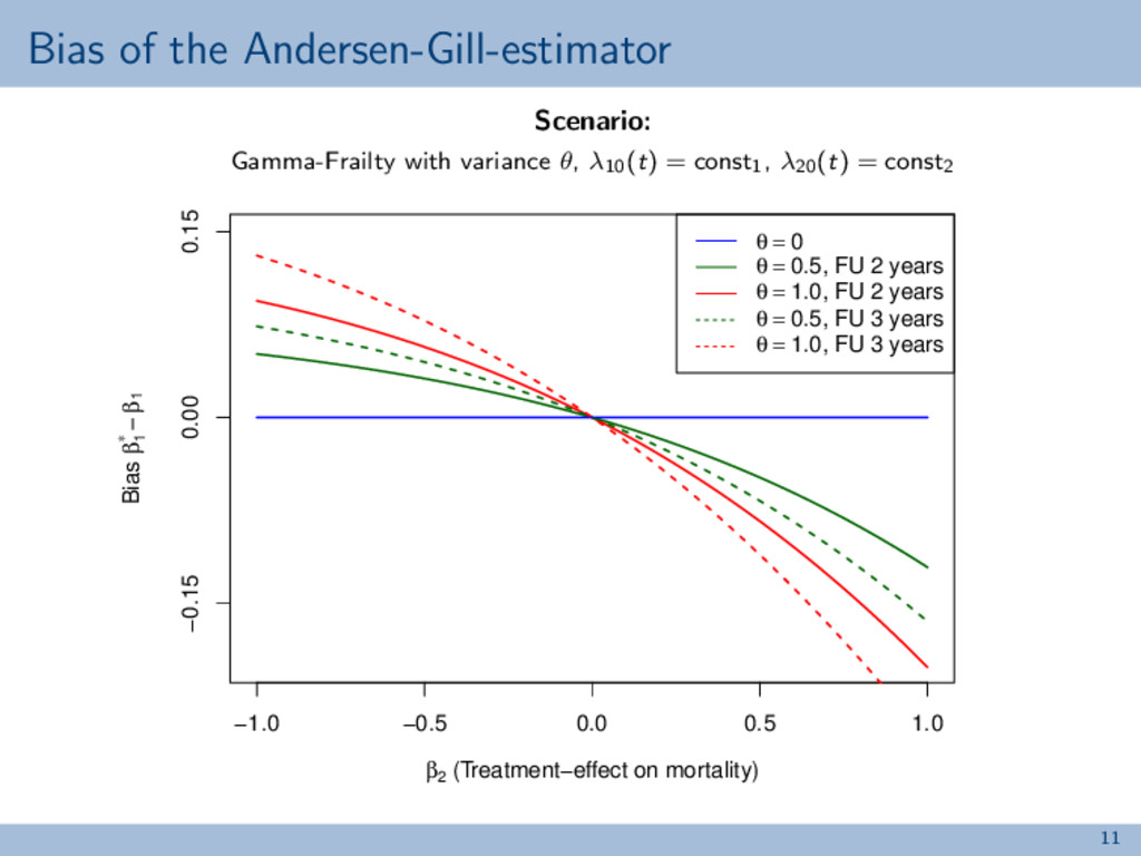
7. Main results The Least False Parameter βAG 1 β∗ 1 (Andersen-Gill-estimator) (Least False Parameter) PJoint Frailty 1. 2. The Least False Parameter β∗ 1 is the root of the function f (c) = ∞ 0 ¯ y(0)(t)¯ y(1)(t) ¯ y(0)(t) + ¯ y(1)(t) exp(c) λ1 (t|x = 1) − exp(c)λ1 (t|x = 0) dt where ¯ y(i)(t) = P(X = i, D > t, C > t). Asymptotic bias of βAG 1 depends on: - Frailty-distribution - Censoring distribution - Treatment-effects - Baseline-hazards 7
8. Bias of the Andersen-Gill-estimator Scenario: Gamma-Frailty with variance θ, λ10(t) = const1, λ20(t) = const2 −1.0 −0.5 0.0 0.5 1.0 β2 (Treatment−effect on mortality) Bias β 1 ∗ − β1 −0.15 0.00 0.15 θ = 0 8
9. Bias of the Andersen-Gill-estimator Scenario: Gamma-Frailty with variance θ, λ10(t) = const1, λ20(t) = const2 −1.0 −0.5 0.0 0.5 1.0 β2 (Treatment−effect on mortality) Bias β 1 ∗ − β1 −0.15 0.00 0.15 θ = 0 θ = 0.5, FU 2 years 9
10. Bias of the Andersen-Gill-estimator Scenario: Gamma-Frailty with variance θ, λ10(t) = const1, λ20(t) = const2 −1.0 −0.5 0.0 0.5 1.0 β2 (Treatment−effect on mortality) Bias β 1 ∗ − β1 −0.15 0.00 0.15 θ = 0 θ = 0.5, FU 2 years θ = 1.0, FU 2 years 10
11. Bias of the Andersen-Gill-estimator Scenario: Gamma-Frailty with variance θ, λ10(t) = const1, λ20(t) = const2 −1.0 −0.5 0.0 0.5 1.0 β2 (Treatment−effect on mortality) Bias β 1 ∗ − β1 −0.15 0.00 0.15 θ = 0 θ = 0.5, FU 2 years θ = 1.0, FU 2 years θ = 0.5, FU 3 years θ = 1.0, FU 3 years 11
12. Val-HeFT-trial results Analysis of Val-HeFT-data: Marginal Models vs. Joint Frailty Model 0.6 0.8 1.0 1.2 1.4 unpublished result: not shown unpublished result: not shown Hazard Ratio (recurrent) AG−Model JF−Model Hazard Ratio (death) Cox−Model JF−Model Hazard Ratio Results from Cohn, J.N. (2001): A Randomized Trial of the Angiotensin-Receptor Blocker Valsartan in Chronic Heart Failure. NEJM, No. 345, p. 1667-1675, additional unpublished results from Dr. M. Akacha (Novartis Pharma) 12
13. Summary Direction of treatment-effect on mortality (β2 ) Bias-Direction of marginal recurrent effect estimator (βAG 1 ) β2 < 0 β∗ 1 > β1 (Bias positive) β2 = 0 β∗ 1 = β1 (No bias) β2 > 0 β∗ 1 < β1 (Bias negative) = Analytically shown for Gamma-Frailty = Analytically shown for every Frailty-distribution 13