Christopher Cheyne

Transcript

1. Improving prognostic accuracy of diabetic retinopathy using multivariate techniques Christopher P Cheyne*, David M Hughes, Arnošt Komárek, Deborah M Broadbent, Amu Wang, Mehrdad Mobayen-Rahni, Ayesh Alshukri, Irene M Stratton, Anthony C Fisher, Jiten Vora, Marta García-Fiñana, Simon P Harding *Department of Biostatistics, University of Liverpool, UK. SAM 2017
2. Contents • Clinical motivation • Dynamic longitudinal discriminant approach • Application to diabetic retinopathy data • Future work
3. Clinical Motivation
4. Diabetic Retinopathy Screening • Patients with diabetes are at risk of developing STDR • Screened annually at a considerable cost to the NHS • Important to identify patients with a higher risk in order to tailor the screening intervals • Patients with higher risk should be screened more often than once per year • The low risk group (the majority) could be screened less frequently than annually • Benefits: Personalised approach, reduction of NHS costs and a decreased burden on patients and clinicians
5. ISDR • NIHR 2014-2019: Introducing personalised risk based intervals in Screening for Diabetic Retinopathy (ISDR), PI: Prof. Harding • Data collected over 7 years (2009-2015) from about 21000 patients with diabetes • Demographic, clinical and ocular risk factors recorded over time (longitudinal markers of different type)
6. Data Sources: Flowchart ISDR Data Ware- house EMIS web (CCG) DIABOLOS (Screening Programme) 1991- Demographic and systemic risk factors Demographic and retinopathy grading (photography) Visual acuity Demographic and retinopathy grading (photography, biomicroscopy) Visual acuity Laboratory test results Risk factors IPM Opt-out Appointments, attendance, Treatment episodes Death Patient opt-out from ISDR Health economics analysis Risk Calculation Engine RCT Web-based grading capture (Hospital Eye Service) 2013- Clinical data validation (inc. query management) internal validation ICE Retinopathy grading (biomicroscopy) Visual acuity, cause of visual impairment Observational cohort study Demographic data Appointments HE dataset Validation dataset Full dataset Risk covariates and outcomes Randomisation Inclusion / exclusion OptoMize (Screening Programme) 2013- ORION (Screening Programme) 1995-2013
7. Data Sources: Example Variables EMIS • Gender • Date of Birth • Earliest Date of Diagnosis of Diabetes • Latest Diagnosis of Diabetes (Type) • Ethnicity • Height • GP Code • HbA1c • Total Cholesterol • LDL Cholesterol • HDL Cholesterol • Diastolic Blood Pressure • Systolic Blood Pressure • eGFR • Triglycerides • ACR • Smoking Status • Weight • Lipid Lowering Treatment (YT/N) • Anti-diabetic treatment (Y/N) • Insulin Treatment (Y/N) • … OptoMize • Screening Appointment Date • Retinopathy Score (R0/1/2/3) – Left Eye – Right Eye • Maculopathy Score (M0/1) – Left Eye – Right Eye • Attendance at screening appointment • … DIABOLOS • Biomicroscopy Date • Best Visual Acuity – Left Eye – Right Eye • Feature Specific Grading – Left Eye – Right Eye • Retinopathy Level – Left Eye – Right Eye • Maculopathy Level – Left Eye – Right Eye • Laser (PRP, Focal or Grid) – Left Eye – Right Eye • …
8. Data Challenges • Input errors • Inconsistency across databases • Data from patients deceased prior to the start of the study not accessible • Accuracy of duration of diabetes • Code errors • STDR event date unknown (interval censored data) • Missingness • …
9. Data Sources: Timeline Covariate Information 1991 2016 2009 Cohort Study Data Timeframe to 2016 EMIS Screening Information OptoMize 2013 2005 DIABOLOS 1995 Biomicroscopy Information DIABOLOS Estimated Numbers screened 100 1000 6000 15000 18000 1994 2001 2005 SOLID LINE: In Data Warehouse ORION Some Data in OptoMize DOTTED LINE : Not In Data Warehouse KEY:
10. Data Linkage: Patient Timelines 2006 2009 2012 2007 2008 2010 2011 2013 2014 Attended Screening Appointment (OptoMize) Biomicroscopy (DIABOLOS) KEY: GP-Recorded Covariate (EMIS): Length of arrow represents the number of distinct, different dates over a 3-month period (Jan-Mar/Apr-Jun/Jul-Sep/ Oct-Dec) 1 2 3 4 5 6 7 Non-attended Screening Appointment (OptoMize/ORION)
11. Different Ways to Merge the Data Key questions to ask: • What should each row represent? • What are the key ‘event’ dates? This should relate to your research questions and how you want to best answer them. Some possibilities: (1) Each row is a screening episode/biomicroscopy/DR treatment and time-varying covariates are attached using the value recorded closest to each of those dates. (2) Same as (1), but assign an average value for each covariate within 1 year prior to se/bio/treatment. (3) Every GP visit date is also included as a separate row. This would require some linkage to se/bio/treatment (e.g. no. of days prior to next se/bio/treatment). ISDR
12. Data Linkage: One Example Patient ID Date Ret_L Mac_L Ret_R Mac_R 1539 10/09/2013 R0 M0 R0 M0 1539 25/11/2014 R1 M0 R1 M0 1539 06/01/2016 R2 M0 R1 M0 1539 30/03/2016 NA NA NA NA Sex Age M 53 M 54 M 55 M 55 … … … SBP HbA1c HDL 132 87 1 112 81 1 122 67 1 122 67 1 … … … LEVABEST REVABEST STDR NA NA NA NA NA NA NA NA NA 0 -0.08 Y … … … Optomize: Screening Data EMIS: Static (non-time varying) GP Data EMIS: Time varying GP Data DIABOLOS: Biomicroscopy Data
13. Data Linkage: Screening Episode
14. Dynamic Longitudinal Approach
15. DiALog MRC 2014-2017: Discriminant Function Analysis for Longitudinal Data, PI: M. García-Fiñana • Discriminant approach using multiple longitudinal markers of different types • Current discriminant approaches based on – a single longitudinal marker – multiple continuous markers using multivariate mixed models – continuous and binary markers but normality of the random effects assumed
16. Definitions • We consider G ≥ 2 groups, R ≥ 1 markers and N patients. • The time points at which biomarkers are measured may be different between biomarkers • Yr,j is the observation of the rth marker on a particular patient at time tr;j ; j = 1, … , nr . • Distribution of each marker may depend on covariates (time, age, sex, etc.)
17. Multivariate Generalized Linear Mixed Model • To allow for different types we model each marker using a generalised linear mixed model ℎ" #$ Y",( |b, = = x ",( /0 " / + z ",( /0 b" (1) • hr is a link function used depending on the type of longitudinal marker. • αr is a vector of fixed parameters for marker r. • br is a vector of random effects for marker r (i.e subjectspecific parameters). • x ",( /0 and z ",( /0 are covariate vectors used in the model for group g
18. Joint Distribution of the Random Effects • The dependence between markers is captured by the joint distribution of the random effects br • The most common assumption is that the random effects follow a Normal distribution: b | = ~ , D (2) • This assumption can be difficult to verify and additional flexibility can be achieved by allowing a mixture of Normal distributions: b | = ~ ∑ ; / <= ;>$ ; /, D; / (3)
19. Longitudinal Discriminant Analysis • Fit MGLMM to data in each prognostic group g, g = 0, ... , G–1 to obtain MCMC parameter estimates. • Use the fitted models to derive the discriminant rule that assigns a new patient to a group. • The probability that the new patient with Yi is from group g is: • The prior probability of being in group g is denoted πg . • Assign new patients to the STDR group if: @ , = E= G =,HIJ ∑ EK G K,HIJ LMN KOP (4) @ , >
20. Application to Diabetic Retinopathy Data
21. Diabetic Retinopathy Example • We included 15,601 patients who were screened between February 2009 and April 2015 for diabetic retinopathy • 6 longitudinal markers considered (HbA1c, cholesterol, retinopathy grading R/L, eGFR, SBP) • 479 patients had STDR within the observation period. • 70% of the patients in each group to train MGLMMs (one for each group). • 30% of patients to test the classification accuracy.
23. Profile of Longitudinal Markers
24. Profile of Longitudinal Markers (cont’d)
25. Work in Progress... • An implementation of the methods described here have now been added to the package mixAK (Komárek and Komárková, 2014) of the R software
26. Future Work
27. Future Work • Identification of the most accurate discriminant model (including external validation) • Can we identify the ideal timing of the next screening interval? • Inclusion of categorical longitudinal markers within this framework • ...
28. Acknowledgements • We are grateful for the support of the ISDR team • We are grateful to the patients involved in ISDR • MRC Dialog Research project MR/L010909/1 • NIHR ISDR Research project RP-DG-1210-12016
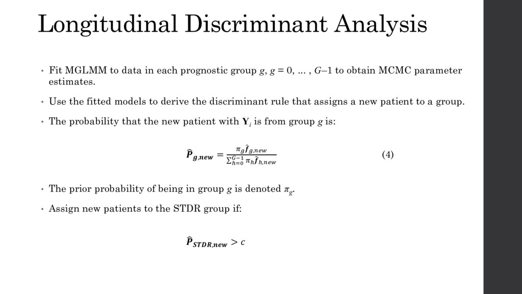
29. References • Brant, L.J., Sheng S.L., Morrell, C.H., Verbeke, G. N., Lesaffre, E. and Carter, H. B. (2003) Screening for prostate cancer by using random-effects models. Journal of the Royal Statistical Society: Series A, 166(1):51–62 • Fieuws, S., Verbeke, G., Maes, B., and Vanrenterghem, Y. (2008) Predicting renal graft failure using multivariate longitudinal profiles. Biostatistics, 9(3):419–431 • Komárek, A., Hansen, B.E., Kuiper, E.M.M., van Buuren, H.R., and Lesaffre, E. (2010) Discriminant analysis using a multivariate linear mixed model with a normal mixture in the random effects distribution. Statistics in medicine, 29(30):3267–3283. • Lix, L.M., and Sajobi, T.T. (2010) Discriminant analysis for repeated measures data: a review. Frontiers in psychology, 1, Article 146. • Marshall, G., De la Cruz-Mesía, R., Quintana, F.A., and Baron, A.E. (2009) Discriminant Analysis for Longitudinal Data with Multiple Continuous Responses and Possibly Missing Data. Biometrics 65:69–80. • Morrell, C.H., Brant, L.J., Sheng, S.L., and Metter, E. J. (2012) Screening for prostate cancer using multivariate mixed-effects models. Journal of applied statistics, 39(6):1151– 1175. • Tomasko, L., Helms, R.W. and Snapinn, S.M. (1999) A discriminant analysis extension to mixed models. Statistics in medicine, 18(10):1249–1260. • Wernecke, K-D., Kalb, G., Schink T., and Wegner, B. (2004) A mixed model approach to discriminant analysis with longitudinal data. Biometrical journal, 46(2):246–254.