Hannah Lennon

Transcript

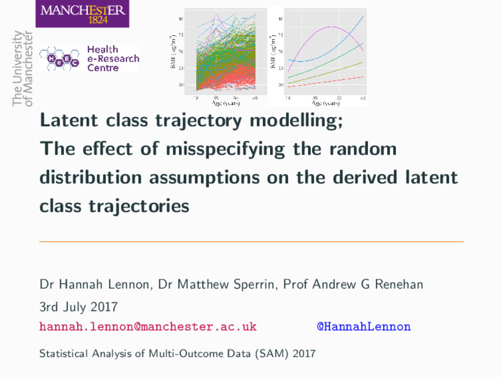
1. Latent class trajectory modelling; The effect of misspecifying the random distribution assumptions on the derived latent class trajectories Dr Hannah Lennon, Dr Matthew Sperrin, Prof Andrew G Renehan 3rd July 2017 hannah.lennon@manchester.ac.uk @HannahLennon Statistical Analysis of Multi-Outcome Data (SAM) 2017
2. Introduction to latent class linear mixed models 1/14
3. Introduction to latent class linear mixed models 1/14
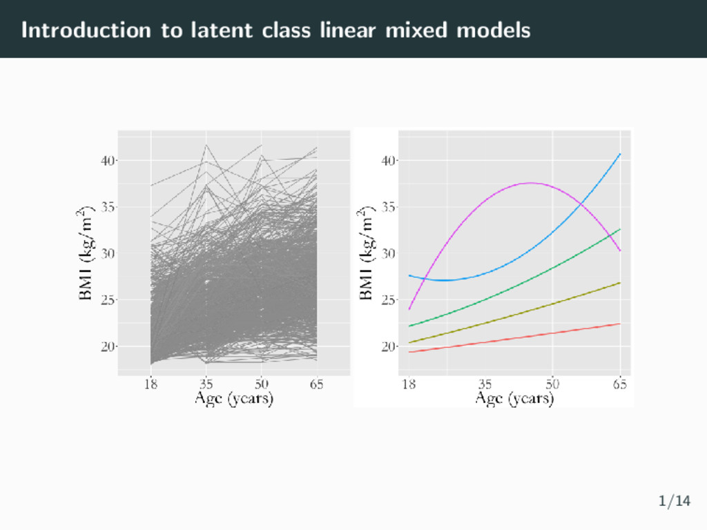
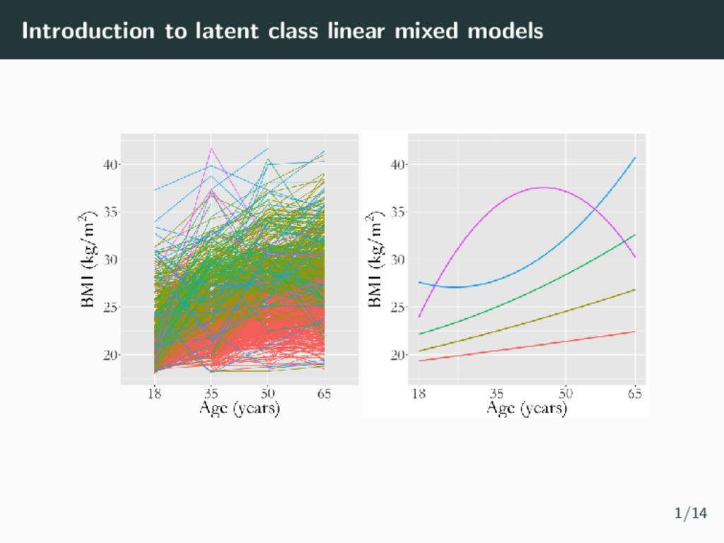
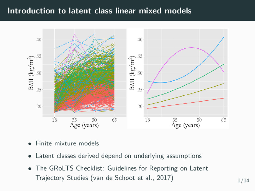
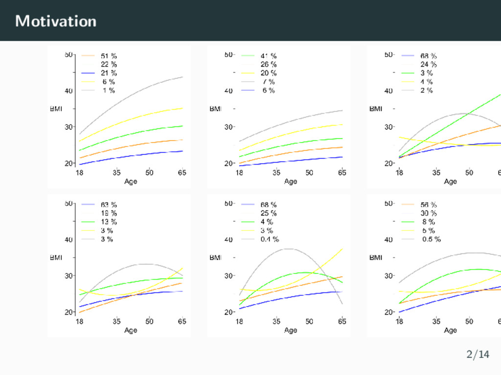
4. Introduction to latent class linear mixed models • Finite mixture models • Latent classes derived depend on underlying assumptions • The GRoLTS Checklist: Guidelines for Reporting on Latent Trajectory Studies (van de Schoot et al., 2017) 1/14
5. Motivation 2/14
6. Structure of Talk Introduction Methods Study I Study II Take Home Messages 3/14
7. Structure of Talk Introduction to latent class linear mixed models Methods A simulation study under various variance-covariance matrix scenarios Simulation Study I Varying DGP (sample sizes and class proportions) under one model fit Simulation Study II Varying models: under one DGP Take Home Messages 3/14
8. Introduction
9. The latent class linear mixed model The model is an extension of the linear mixed model of Laird & Ware (1982) for individuals i = 1, . . . , N at times j = 1, . . . , T, for k = 1, . . . , K classes Yij|ci =k = Xi (tij )βk + Zik (tij )uik + wk (tij ) + εijk , (1) εij iid ∼ N(0, R). where both the fixed effects and the distribution of the random effects can be class-specific. 4/14
10. The latent class linear mixed model The model is an extension of the linear mixed model of Laird & Ware (1982) for individuals i = 1, . . . , N at times j = 1, . . . , T, for k = 1, . . . , K classes Yij|ci =k = Xi (tij )βk + Zik (tij )uik + wk (tij ) + εijk , (1) εij iid ∼ N(0, R). where both the fixed effects and the distribution of the random effects can be class-specific. 4/14
11. The latent class linear mixed model The model is an extension of the linear mixed model of Laird & Ware (1982) for individuals i = 1, . . . , N at times j = 1, . . . , T, for k = 1, . . . , K classes Yij|ci =k = Xi (tij )βk + Zik (tij )uik + wk (tij ) + εijk , (1) εij iid ∼ N(0, R). where both the fixed effects and the distribution of the random effects can be class-specific. 4/14
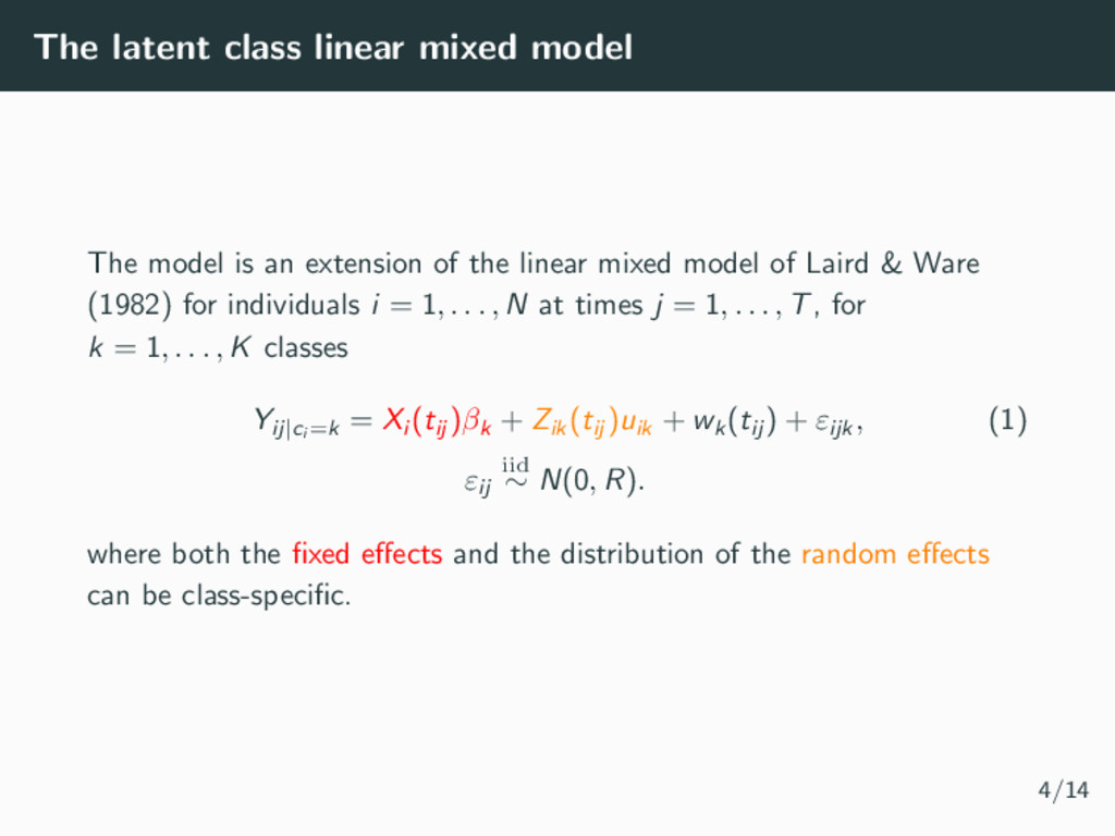
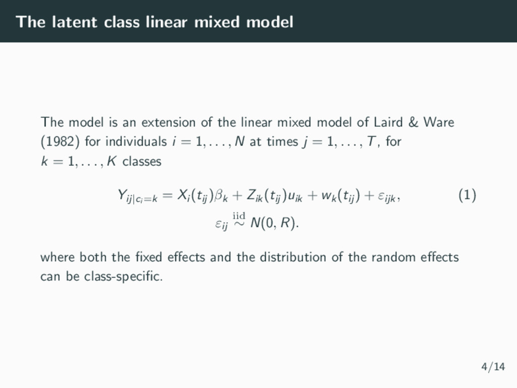
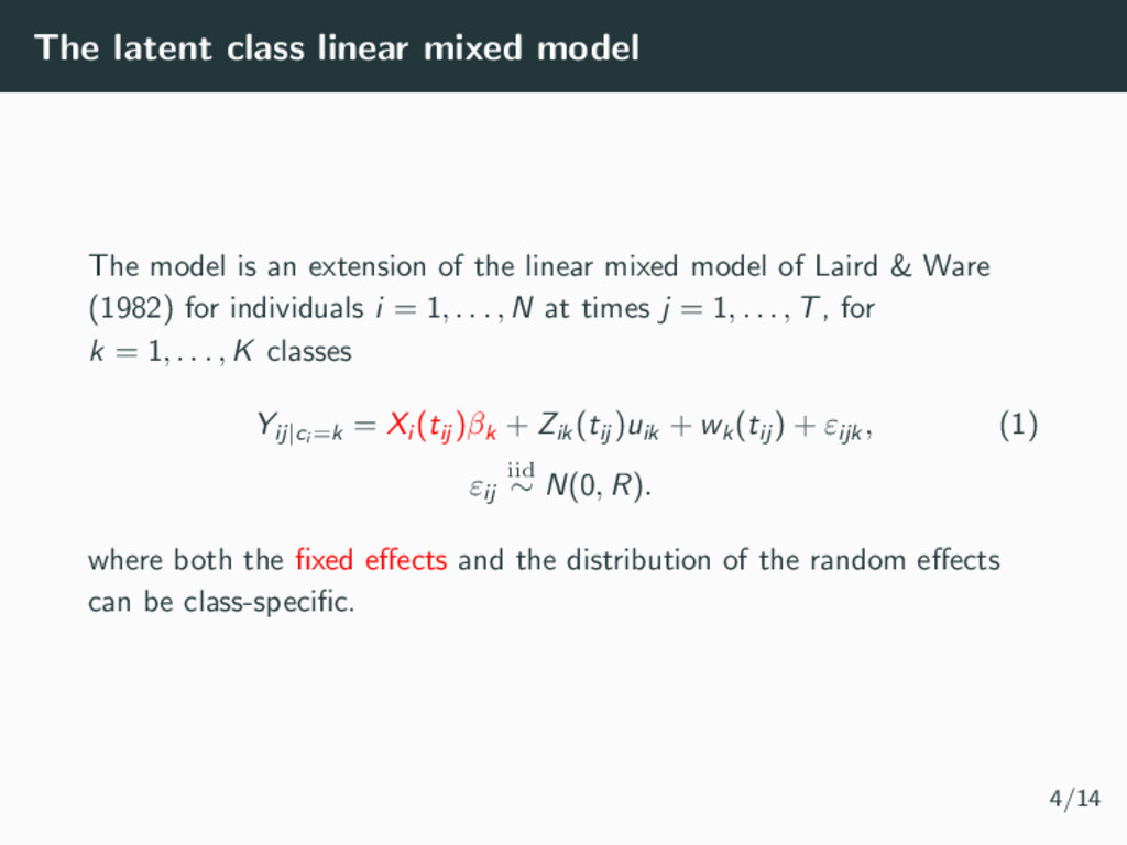
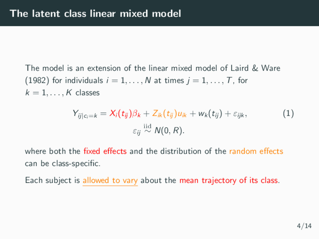
12. The latent class linear mixed model The model is an extension of the linear mixed model of Laird & Ware (1982) for individuals i = 1, . . . , N at times j = 1, . . . , T, for k = 1, . . . , K classes Yij|ci =k = Xi (tij )βk + Zik (tij )uik + wk (tij ) + εijk , (1) εij iid ∼ N(0, R). where both the fixed effects and the distribution of the random effects can be class-specific. Each subject is allowed to vary about the mean trajectory of its class. 4/14
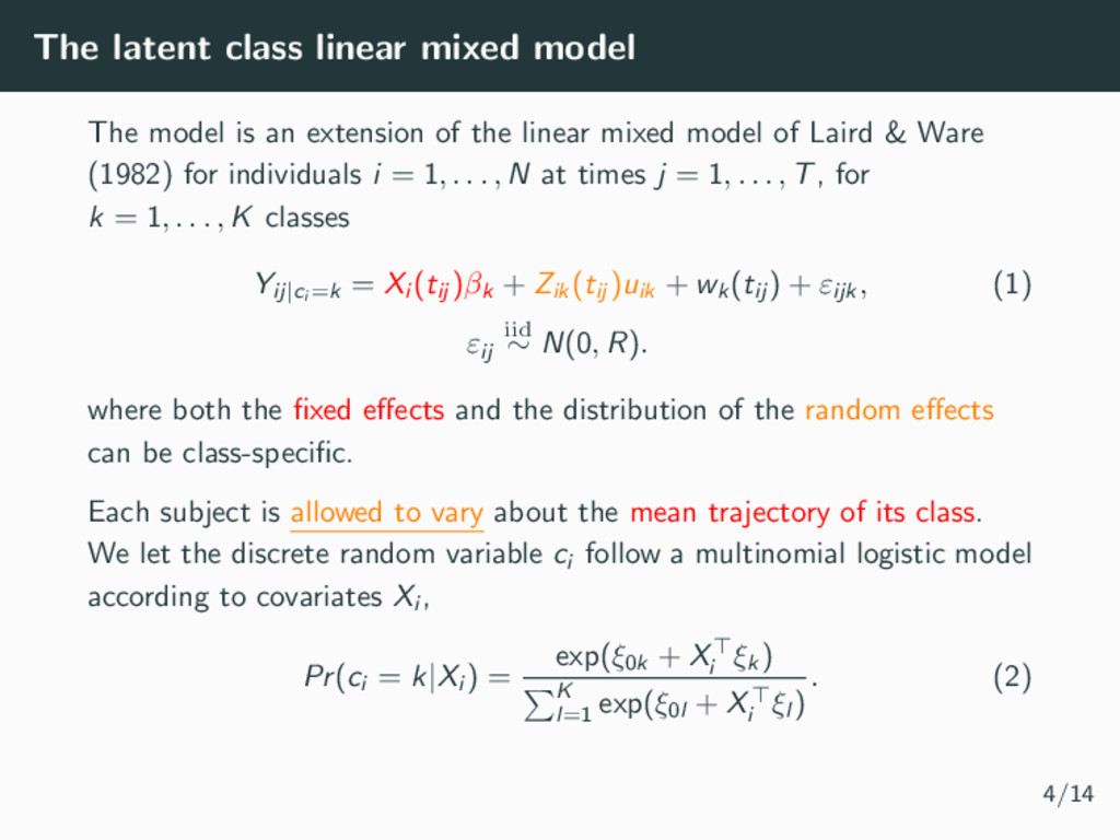
13. The latent class linear mixed model The model is an extension of the linear mixed model of Laird & Ware (1982) for individuals i = 1, . . . , N at times j = 1, . . . , T, for k = 1, . . . , K classes Yij|ci =k = Xi (tij )βk + Zik (tij )uik + wk (tij ) + εijk , (1) εij iid ∼ N(0, R). where both the fixed effects and the distribution of the random effects can be class-specific. Each subject is allowed to vary about the mean trajectory of its class. We let the discrete random variable ci follow a multinomial logistic model according to covariates Xi , Pr(ci = k|Xi ) = exp(ξ0k + Xi ξk ) K l=1 exp(ξ0l + X i ξl ) . (2) 4/14
14. Methods
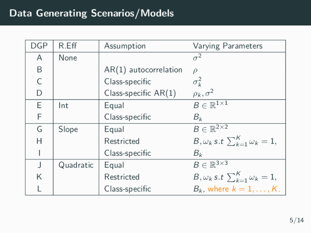
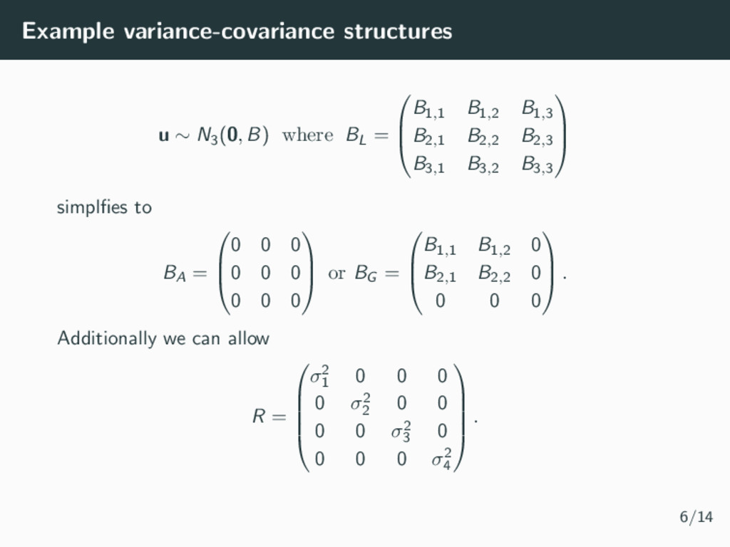
15. Data Generating Scenarios/Models DGP R.Eff Assumption Varying Parameters A None σ2 B AR(1) autocorrelation ρ C Class-specific σ2 k D Class-specific AR(1) ρk , σ2 E Int Equal B ∈ R1×1 F Class-specific Bk G Slope Equal B ∈ R2×2 H Restricted B, ωk s.t K k=1 ωk = 1, I Class-specific Bk J Quadratic Equal B ∈ R3×3 K Restricted B, ωk s.t K k=1 ωk = 1, L Class-specific Bk , where k = 1, . . . , K. 5/14
16. Example variance-covariance structures u ∼ N3 (0, B) where BL =    B1,1 B1,2 B1,3 B2,1 B2,2 B2,3 B3,1 B3,2 B3,3    simplfies to BA =    0 0 0 0 0 0 0 0 0    or BG =    B1,1 B1,2 0 B2,1 B2,2 0 0 0 0    . Additionally we can allow R =      σ2 1 0 0 0 0 σ2 2 0 0 0 0 σ2 3 0 0 0 0 σ2 4      . 6/14
17. Study I
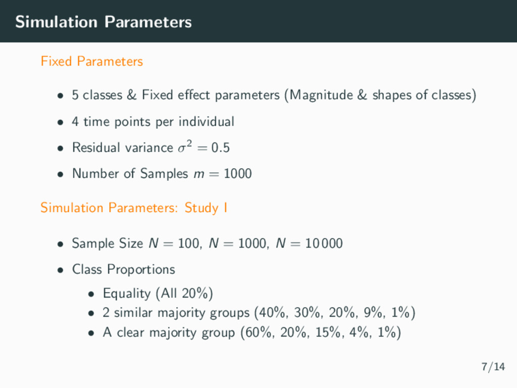
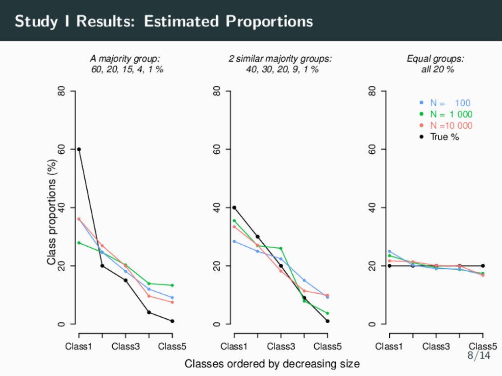
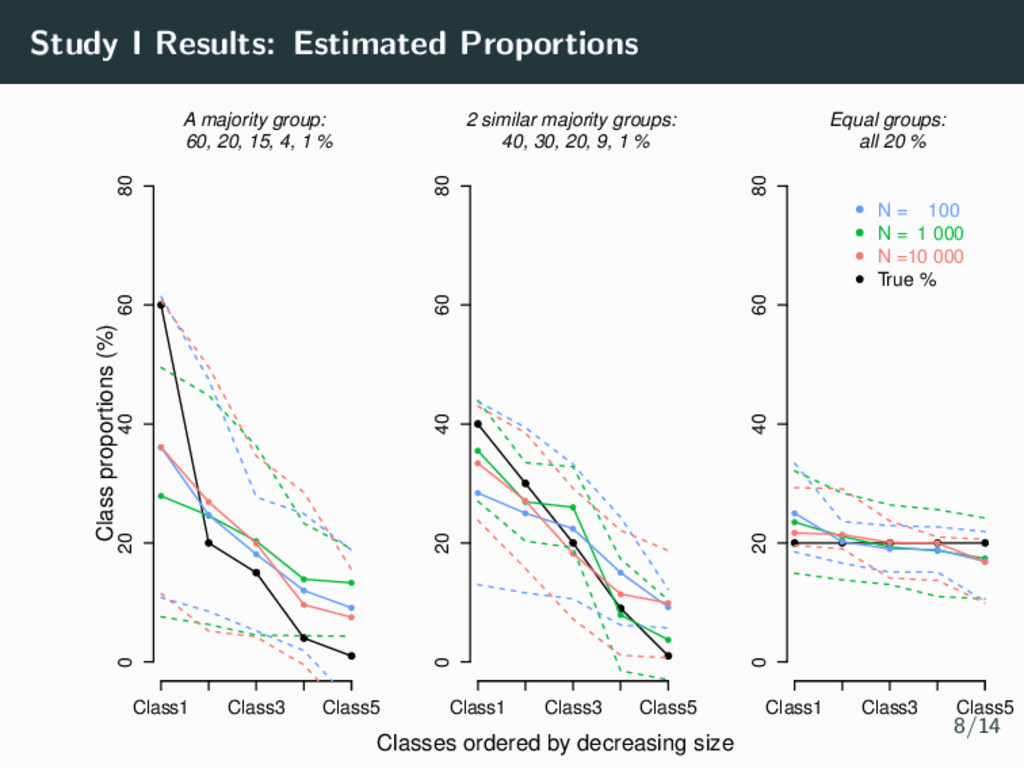
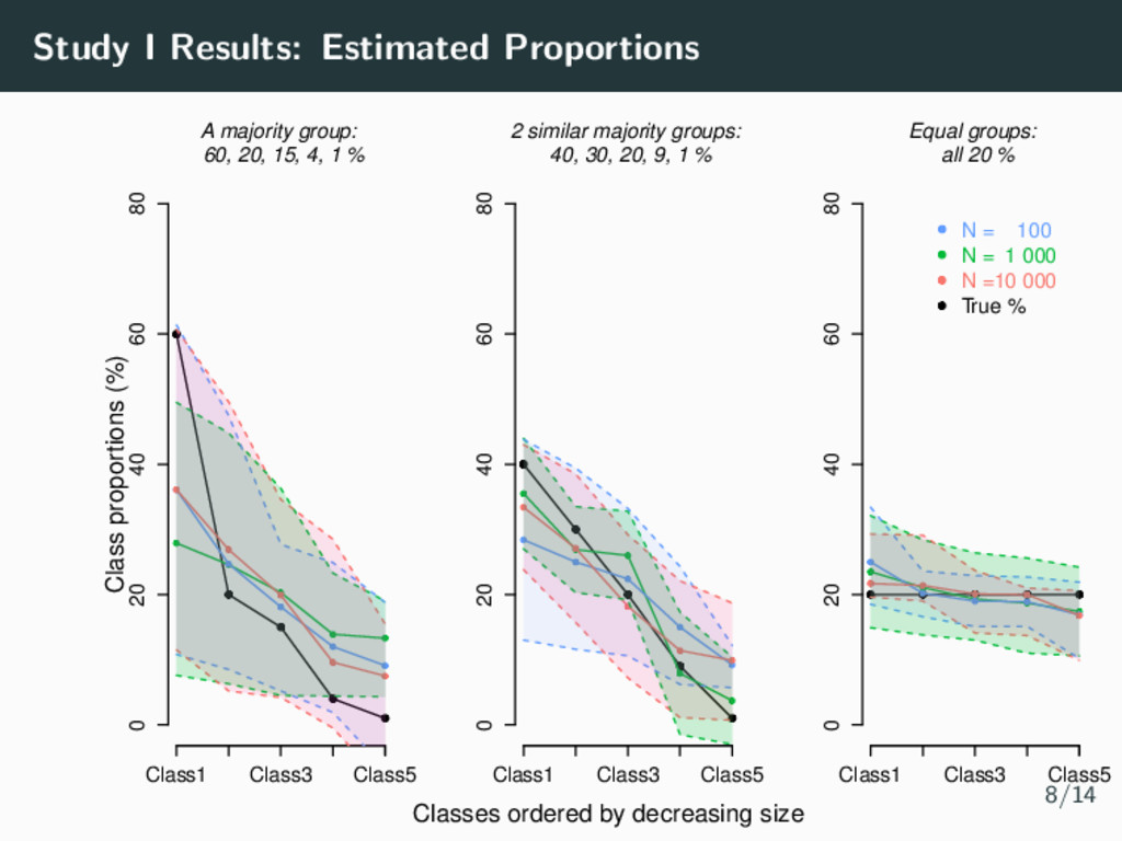
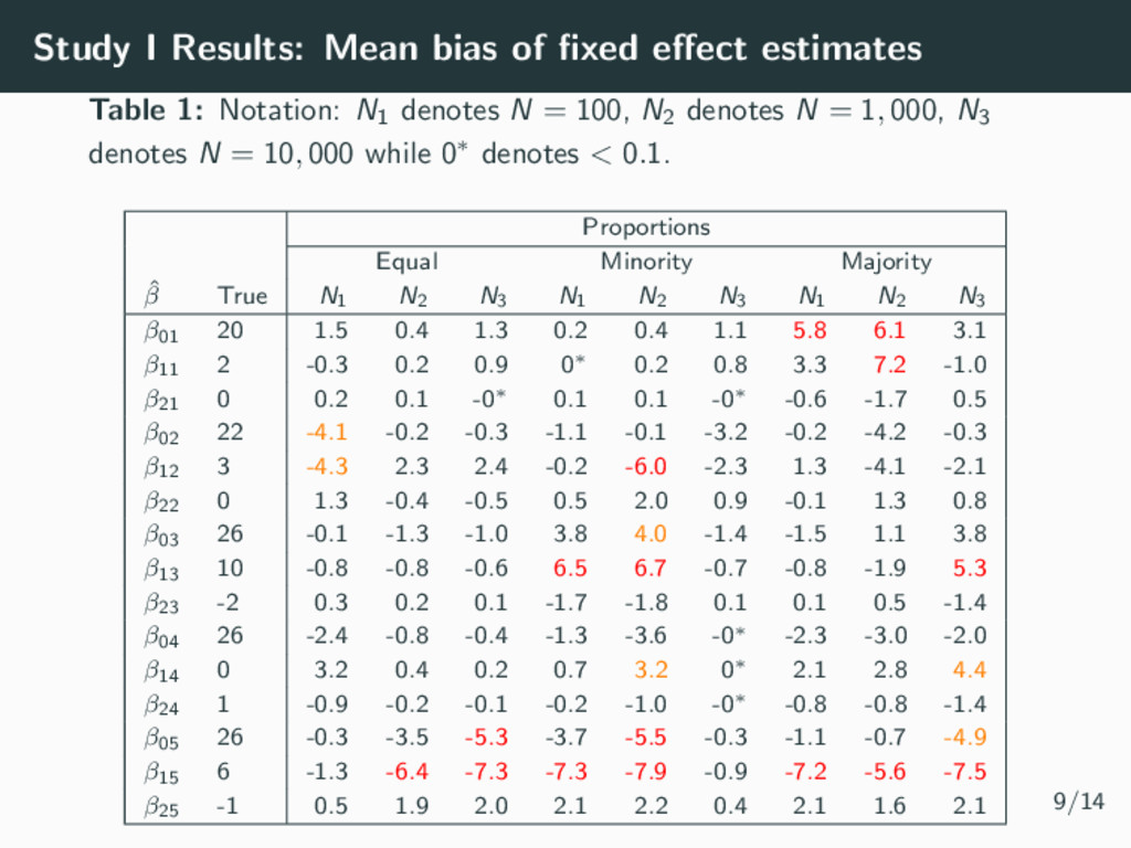
18. Simulation Parameters Fixed Parameters • 5 classes & Fixed effect parameters (Magnitude & shapes of classes) • 4 time points per individual • Residual variance σ2 = 0.5 • Number of Samples m = 1000 Simulation Parameters: Study I • Sample Size N = 100, N = 1000, N = 10 000 • Class Proportions • Equality (All 20%) • 2 similar majority groups (40%, 30%, 20%, 9%, 1%) • A clear majority group (60%, 20%, 15%, 4%, 1%) 7/14
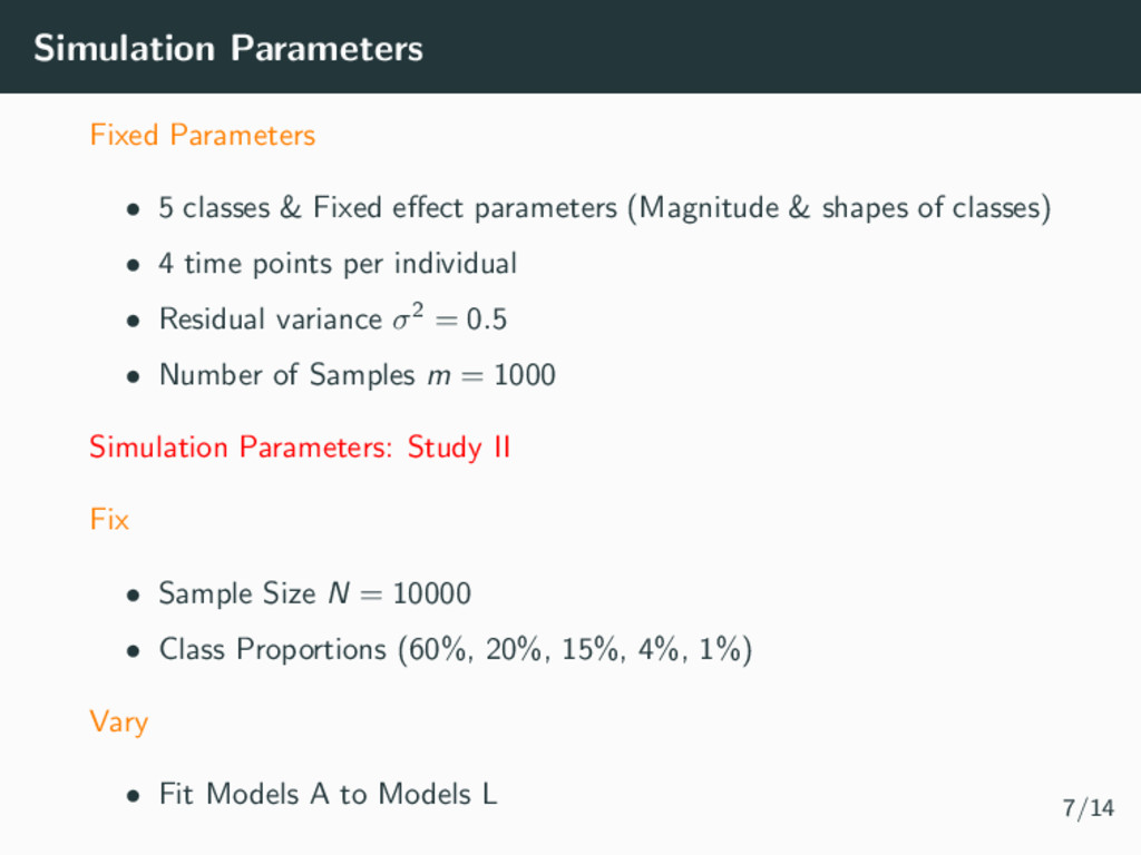
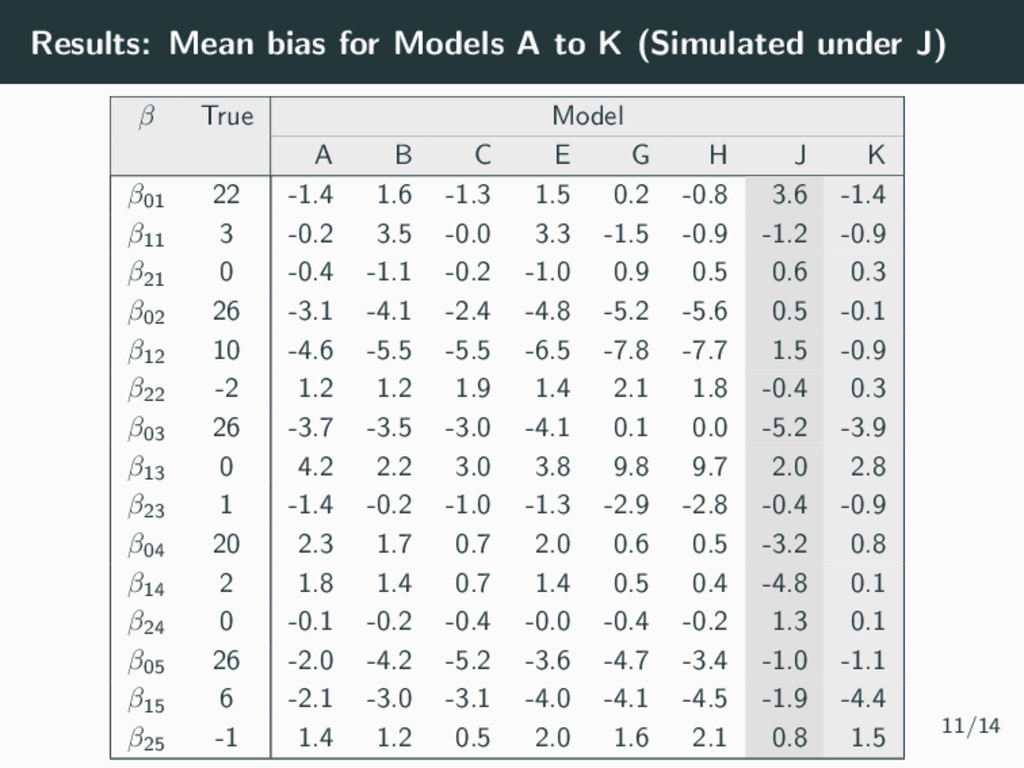
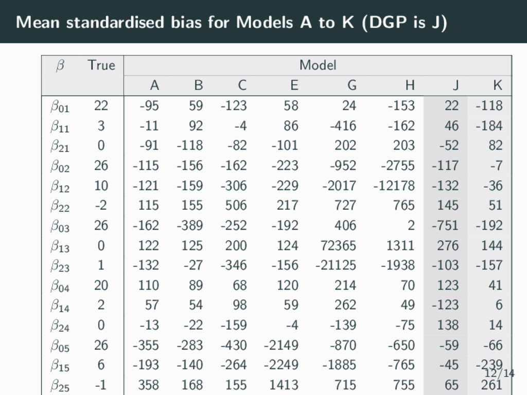
19. Simulation Parameters Fixed Parameters • 5 classes & Fixed effect parameters (Magnitude & shapes of classes) • 4 time points per individual • Residual variance σ2 = 0.5 • Number of Samples m = 1000 Simulation Parameters: Study II Fix • Sample Size N = 10000 • Class Proportions (60%, 20%, 15%, 4%, 1%) Vary • Fit Models A to Models L 7/14
20. Study I Results: Estimated Proportions q q q q q Class1 Class3 Class5 0 20 40 60 80 q q q q q q q q q q q q q q q A majority group: 60, 20, 15, 4, 1 % q q q q q Class1 Class3 Class5 0 20 40 60 80 q q q q q q q q q q q q q q q 2 similar majority groups: 40, 30, 20, 9, 1 % q q q q q Class1 Class3 Class5 0 20 40 60 80 q q q q q q q q q q q q q q q Equal groups: all 20 % q q q q N = 100 N = 1 000 N =10 000 True % Classes ordered by decreasing size Class proportions (%) 8/14
21. Study I Results: Estimated Proportions q q q q q Class1 Class3 Class5 0 20 40 60 80 q q q q q q q q q q q q q q q A majority group: 60, 20, 15, 4, 1 % q q q q q Class1 Class3 Class5 0 20 40 60 80 q q q q q q q q q q q q q q q 2 similar majority groups: 40, 30, 20, 9, 1 % q q q q q Class1 Class3 Class5 0 20 40 60 80 q q q q q q q q q q q q q q q Equal groups: all 20 % q q q q N = 100 N = 1 000 N =10 000 True % Classes ordered by decreasing size Class proportions (%) 8/14
22. Study I Results: Estimated Proportions q q q q q Class1 Class3 Class5 0 20 40 60 80 q q q q q q q q q q q q q q q A majority group: 60, 20, 15, 4, 1 % q q q q q Class1 Class3 Class5 0 20 40 60 80 q q q q q q q q q q q q q q q 2 similar majority groups: 40, 30, 20, 9, 1 % q q q q q Class1 Class3 Class5 0 20 40 60 80 q q q q q q q q q q q q q q q Equal groups: all 20 % q q q q N = 100 N = 1 000 N =10 000 True % Classes ordered by decreasing size Class proportions (%) 8/14
23. Study I Results: Mean bias of fixed effect estimates Table 1: Notation: N1 denotes N = 100, N2 denotes N = 1, 000, N3 denotes N = 10, 000 while 0∗ denotes < 0.1. Proportions Equal Minority Majority ˆ β True N1 N2 N3 N1 N2 N3 N1 N2 N3 β01 20 1.5 0.4 1.3 0.2 0.4 1.1 5.8 6.1 3.1 β11 2 -0.3 0.2 0.9 0∗ 0.2 0.8 3.3 7.2 -1.0 β21 0 0.2 0.1 -0∗ 0.1 0.1 -0∗ -0.6 -1.7 0.5 β02 22 -4.1 -0.2 -0.3 -1.1 -0.1 -3.2 -0.2 -4.2 -0.3 β12 3 -4.3 2.3 2.4 -0.2 -6.0 -2.3 1.3 -4.1 -2.1 β22 0 1.3 -0.4 -0.5 0.5 2.0 0.9 -0.1 1.3 0.8 β03 26 -0.1 -1.3 -1.0 3.8 4.0 -1.4 -1.5 1.1 3.8 β13 10 -0.8 -0.8 -0.6 6.5 6.7 -0.7 -0.8 -1.9 5.3 β23 -2 0.3 0.2 0.1 -1.7 -1.8 0.1 0.1 0.5 -1.4 β04 26 -2.4 -0.8 -0.4 -1.3 -3.6 -0∗ -2.3 -3.0 -2.0 β14 0 3.2 0.4 0.2 0.7 3.2 0∗ 2.1 2.8 4.4 β24 1 -0.9 -0.2 -0.1 -0.2 -1.0 -0∗ -0.8 -0.8 -1.4 β05 26 -0.3 -3.5 -5.3 -3.7 -5.5 -0.3 -1.1 -0.7 -4.9 β15 6 -1.3 -6.4 -7.3 -7.3 -7.9 -0.9 -7.2 -5.6 -7.5 β25 -1 0.5 1.9 2.0 2.1 2.2 0.4 2.1 1.6 2.1 9/14
24. Study I Results: Mean bias of fixed effect estimates Table 1: Notation: N1 denotes N = 100, N2 denotes N = 1, 000, N3 denotes N = 10, 000 while 0∗ denotes < 0.1. Proportions Equal Minority Majority ˆ β True N1 N2 N3 N1 N2 N3 N1 N2 N3 β01 20 1.5 0.4 1.3 0.2 0.4 1.1 5.8 6.1 3.1 β11 2 -0.3 0.2 0.9 0∗ 0.2 0.8 3.3 7.2 -1.0 β21 0 0.2 0.1 -0∗ 0.1 0.1 -0∗ -0.6 -1.7 0.5 β02 22 -4.1 -0.2 -0.3 -1.1 -0.1 -3.2 -0.2 -4.2 -0.3 β12 3 -4.3 2.3 2.4 -0.2 -6.0 -2.3 1.3 -4.1 -2.1 β22 0 1.3 -0.4 -0.5 0.5 2.0 0.9 -0.1 1.3 0.8 β03 26 -0.1 -1.3 -1.0 3.8 4.0 -1.4 -1.5 1.1 3.8 β13 10 -0.8 -0.8 -0.6 6.5 6.7 -0.7 -0.8 -1.9 5.3 β23 -2 0.3 0.2 0.1 -1.7 -1.8 0.1 0.1 0.5 -1.4 β04 26 -2.4 -0.8 -0.4 -1.3 -3.6 -0∗ -2.3 -3.0 -2.0 β14 0 3.2 0.4 0.2 0.7 3.2 0∗ 2.1 2.8 4.4 β24 1 -0.9 -0.2 -0.1 -0.2 -1.0 -0∗ -0.8 -0.8 -1.4 β05 26 -0.3 -3.5 -5.3 -3.7 -5.5 -0.3 -1.1 -0.7 -4.9 β15 6 -1.3 -6.4 -7.3 -7.3 -7.9 -0.9 -7.2 -5.6 -7.5 β25 -1 0.5 1.9 2.0 2.1 2.2 0.4 2.1 1.6 2.1 9/14
25. Study I Results: Mean bias of fixed effect estimates Table 1: Notation: N1 denotes N = 100, N2 denotes N = 1, 000, N3 denotes N = 10, 000 while 0∗ denotes < 0.1. Proportions Equal Minority Majority ˆ β True N1 N2 N3 N1 N2 N3 N1 N2 N3 β01 20 1.5 0.4 1.3 0.2 0.4 1.1 5.8 6.1 3.1 β11 2 -0.3 0.2 0.9 0∗ 0.2 0.8 3.3 7.2 -1.0 β21 0 0.2 0.1 -0∗ 0.1 0.1 -0∗ -0.6 -1.7 0.5 β02 22 -4.1 -0.2 -0.3 -1.1 -0.1 -3.2 -0.2 -4.2 -0.3 β12 3 -4.3 2.3 2.4 -0.2 -6.0 -2.3 1.3 -4.1 -2.1 β22 0 1.3 -0.4 -0.5 0.5 2.0 0.9 -0.1 1.3 0.8 β03 26 -0.1 -1.3 -1.0 3.8 4.0 -1.4 -1.5 1.1 3.8 β13 10 -0.8 -0.8 -0.6 6.5 6.7 -0.7 -0.8 -1.9 5.3 β23 -2 0.3 0.2 0.1 -1.7 -1.8 0.1 0.1 0.5 -1.4 β04 26 -2.4 -0.8 -0.4 -1.3 -3.6 -0∗ -2.3 -3.0 -2.0 β14 0 3.2 0.4 0.2 0.7 3.2 0∗ 2.1 2.8 4.4 β24 1 -0.9 -0.2 -0.1 -0.2 -1.0 -0∗ -0.8 -0.8 -1.4 β05 26 -0.3 -3.5 -5.3 -3.7 -5.5 -0.3 -1.1 -0.7 -4.9 β15 6 -1.3 -6.4 -7.3 -7.3 -7.9 -0.9 -7.2 -5.6 -7.5 β25 -1 0.5 1.9 2.0 2.1 2.2 0.4 2.1 1.6 2.1 9/14
26. Study II
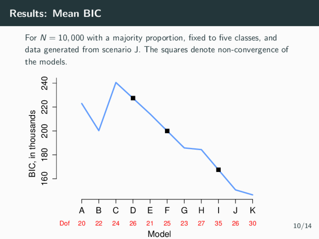
27. Results: Mean BIC For N = 10, 000 with a majority proportion, fixed to five classes, and data generated from scenario J. The squares denote non-convergence of the models. Model Dof 20 22 24 26 21 25 23 27 35 26 30 160 180 200 220 240 A B C D E F G H I J K BIC, in thousands 10/14
28. Results: Mean bias for Models A to K (Simulated under J) β True Model A B C E G H J K β01 22 -1.4 1.6 -1.3 1.5 0.2 -0.8 3.6 -1.4 β11 3 -0.2 3.5 -0.0 3.3 -1.5 -0.9 -1.2 -0.9 β21 0 -0.4 -1.1 -0.2 -1.0 0.9 0.5 0.6 0.3 β02 26 -3.1 -4.1 -2.4 -4.8 -5.2 -5.6 0.5 -0.1 β12 10 -4.6 -5.5 -5.5 -6.5 -7.8 -7.7 1.5 -0.9 β22 -2 1.2 1.2 1.9 1.4 2.1 1.8 -0.4 0.3 β03 26 -3.7 -3.5 -3.0 -4.1 0.1 0.0 -5.2 -3.9 β13 0 4.2 2.2 3.0 3.8 9.8 9.7 2.0 2.8 β23 1 -1.4 -0.2 -1.0 -1.3 -2.9 -2.8 -0.4 -0.9 β04 20 2.3 1.7 0.7 2.0 0.6 0.5 -3.2 0.8 β14 2 1.8 1.4 0.7 1.4 0.5 0.4 -4.8 0.1 β24 0 -0.1 -0.2 -0.4 -0.0 -0.4 -0.2 1.3 0.1 β05 26 -2.0 -4.2 -5.2 -3.6 -4.7 -3.4 -1.0 -1.1 β15 6 -2.1 -3.0 -3.1 -4.0 -4.1 -4.5 -1.9 -4.4 β25 -1 1.4 1.2 0.5 2.0 1.6 2.1 0.8 1.5 11/14
29. Mean standardised bias for Models A to K (DGP is J) β True Model A B C E G H J K β01 22 -95 59 -123 58 24 -153 22 -118 β11 3 -11 92 -4 86 -416 -162 46 -184 β21 0 -91 -118 -82 -101 202 203 -52 82 β02 26 -115 -156 -162 -223 -952 -2755 -117 -7 β12 10 -121 -159 -306 -229 -2017 -12178 -132 -36 β22 -2 115 155 506 217 727 765 145 51 β03 26 -162 -389 -252 -192 406 2 -751 -192 β13 0 122 125 200 124 72365 1311 276 144 β23 1 -132 -27 -346 -156 -21125 -1938 -103 -157 β04 20 110 89 68 120 214 70 123 41 β14 2 57 54 98 59 262 49 -123 6 β24 0 -13 -22 -159 -4 -139 -75 138 14 β05 26 -355 -283 -430 -2149 -870 -650 -59 -66 β15 6 -193 -140 -264 -2249 -1885 -765 -45 -239 β25 -1 358 168 155 1413 715 755 65 261 12/14
30. Take Home Messages
31. Take Home Messages • Latent class linear mixed models can be used to simplify complex longitudinal data into relatively homogeneous sub-populations • Easy to implement in many software packages (R, Stata, SAS, MPlus, LatentGold, etc) and becoming more popular in epidemiology studies 13/14
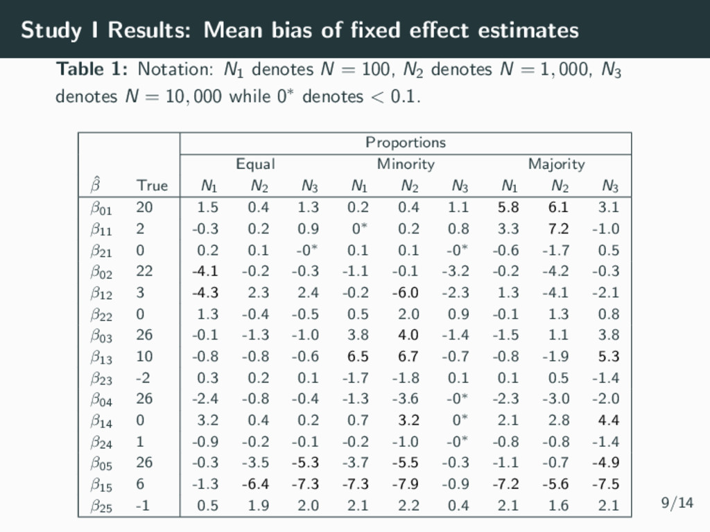
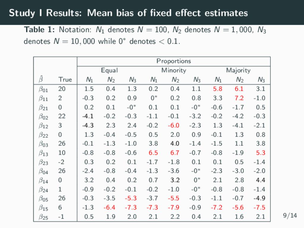
32. Take Home Messages • Latent class linear mixed models can be used to simplify complex longitudinal data into relatively homogeneous sub-populations • Easy to implement in many software packages (R, Stata, SAS, MPlus, LatentGold, etc) and becoming more popular in epidemiology studies • However, the class proportions can be underestimated, affecting the fixed effect estimates and hence the magnitude and size of the trajectories recovered. • The GRoLTS Checklist (2017) can be used to improve reporting standards. • Let’s look deeper into the SEM literature which has already studied many of the emerging questions from epidemiological studies. 13/14
33. Thank you to our funders for financial support 14/14