. . . . . . . . . . . . . . . . . . . . . . . . . . . . . . Introduction Methods Comparison Simulation Study Data Application Discussion Dynamic prediction of event times using longitudinal data Jeremy M.G. Taylor, Krithika Suresh, Alexander Tsodikov Dept of Biostatistics, University of Michigan 3 July 2017 Jeremy Taylor (Dept of Biostatistics, University of Michigan) 3 July 2017 1 / 37
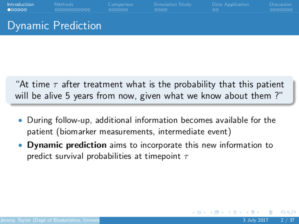
. . . . . . . . . . . . . . . . . . . . . . . . . . . . . . Introduction Methods Comparison Simulation Study Data Application Discussion Dynamic Prediction “At time τ after treatment what is the probability that this patient will be alive 5 years from now, given what we know about them ?” • During follow-up, additional information becomes available for the patient (biomarker measurements, intermediate event) • Dynamic prediction aims to incorporate this new information to predict survival probabilities at timepoint τ Jeremy Taylor (Dept of Biostatistics, University of Michigan) 3 July 2017 2 / 37
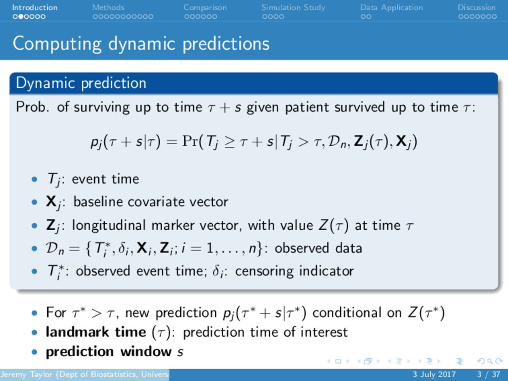
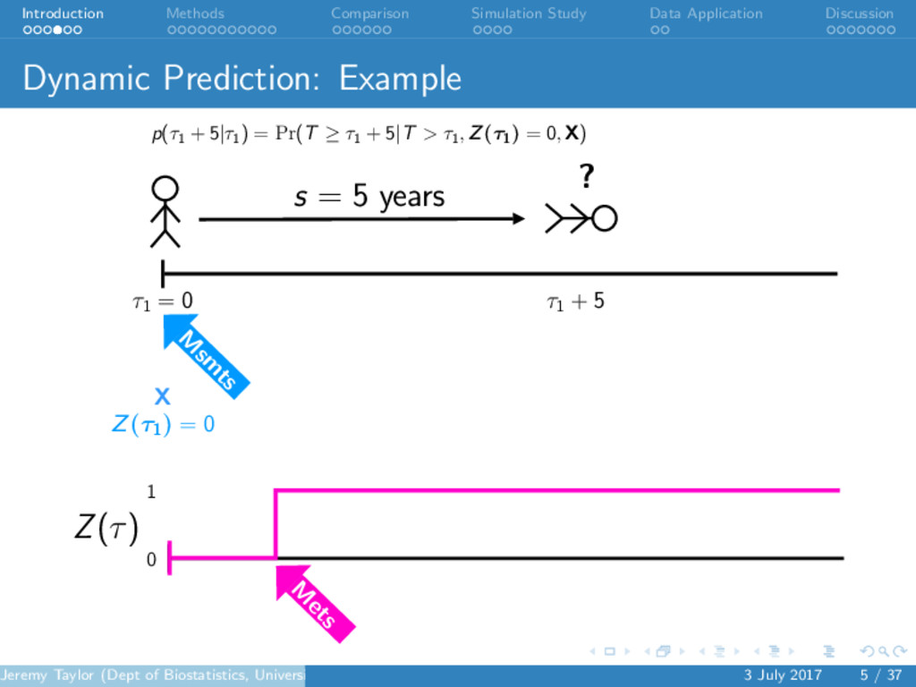
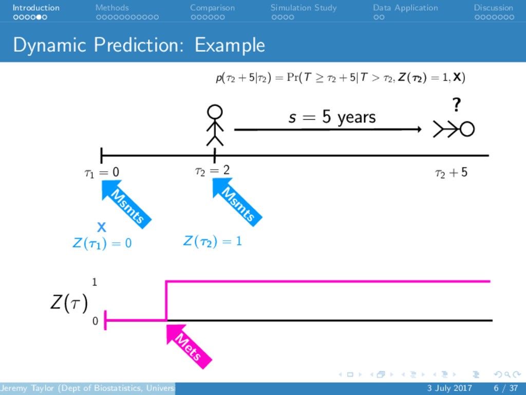
. . . . . . . . . . . . . . . . . . . . . . . . . . . . . . Introduction Methods Comparison Simulation Study Data Application Discussion Computing dynamic predictions Dynamic prediction Prob. of surviving up to time τ + s given patient survived up to time τ: pj (τ + s|τ) = Pr(Tj ≥ τ + s|Tj > τ, Dn, Zj (τ), Xj ) • Tj : event time • Xj : baseline covariate vector • Zj : longitudinal marker vector, with value Z(τ) at time τ • Dn = {T∗ i , δi , Xi , Zi ; i = 1, . . . , n}: observed data • T∗ i : observed event time; δi : censoring indicator • For τ∗ > τ, new prediction pj (τ∗ + s|τ∗) conditional on Z(τ∗) • landmark time (τ): prediction time of interest • prediction window s Jeremy Taylor (Dept of Biostatistics, University of Michigan) 3 July 2017 3 / 37
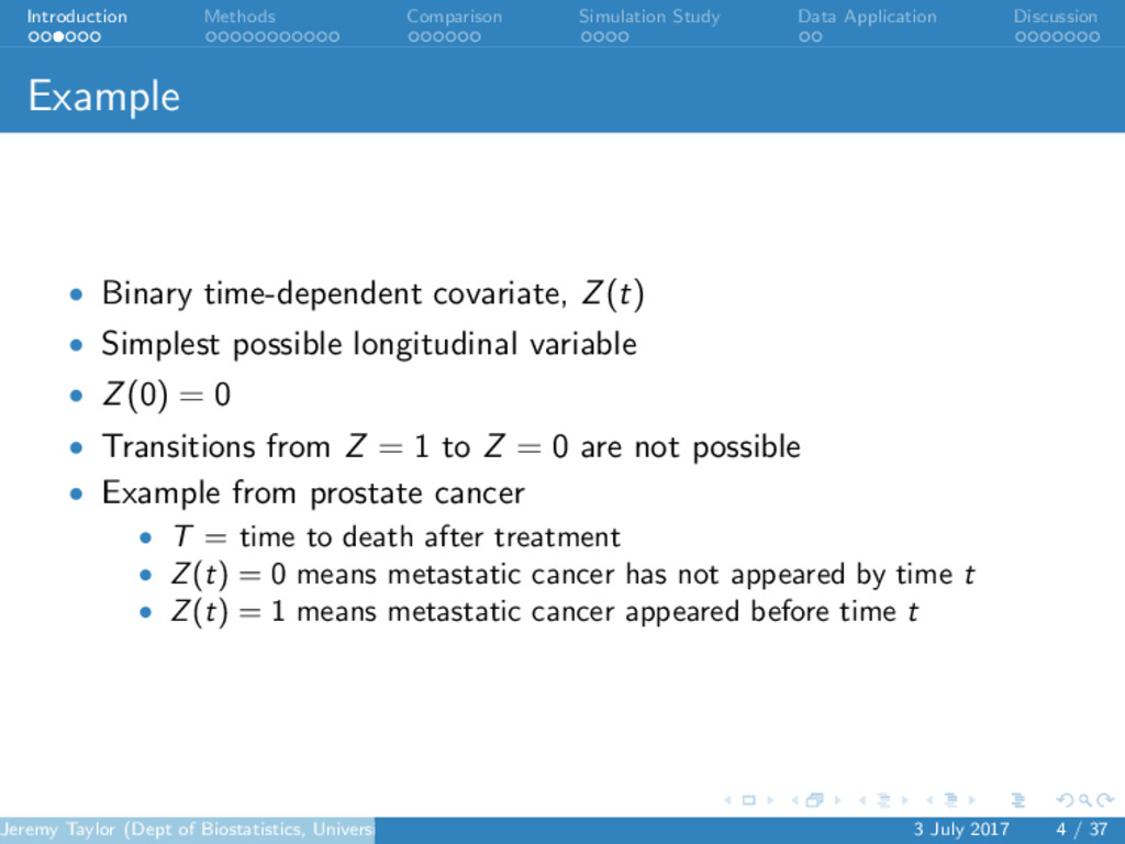
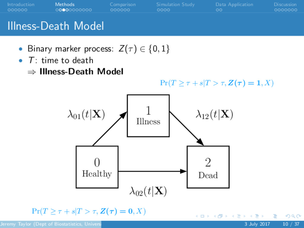
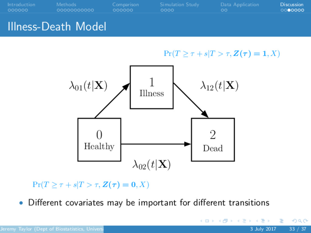
. . . . . . . . . . . . . . . . . . . . . . . . . . . . . . Introduction Methods Comparison Simulation Study Data Application Discussion Example • Binary time-dependent covariate, Z(t) • Simplest possible longitudinal variable • Z(0) = 0 • Transitions from Z = 1 to Z = 0 are not possible • Example from prostate cancer • T = time to death after treatment • Z(t) = 0 means metastatic cancer has not appeared by time t • Z(t) = 1 means metastatic cancer appeared before time t Jeremy Taylor (Dept of Biostatistics, University of Michigan) 3 July 2017 4 / 37
. . . . . . . . . . . . . . . . . . . . . . . . . . . . . . Introduction Methods Comparison Simulation Study Data Application Discussion Methods for Dynamic Prediction 1 Joint Modeling • Taylor et al., (2005, 2013); Rizopoulos et al., (2011, 2013) 2 Landmarking • van Houwelingen (2007), Zheng and Heagerty (2005) • Aim: Compare these two approaches in the context of data with binary Z, (i.e. data from an illness-death model) Jeremy Taylor (Dept of Biostatistics, University of Michigan) 3 July 2017 8 / 37
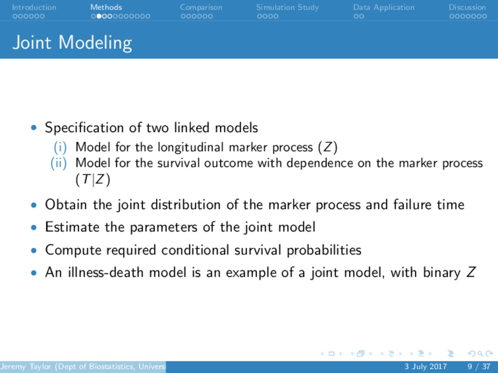
. . . . . . . . . . . . . . . . . . . . . . . . . . . . . . Introduction Methods Comparison Simulation Study Data Application Discussion Joint Modeling • Specification of two linked models (i) Model for the longitudinal marker process (Z) (ii) Model for the survival outcome with dependence on the marker process (T|Z) • Obtain the joint distribution of the marker process and failure time • Estimate the parameters of the joint model • Compute required conditional survival probabilities • An illness-death model is an example of a joint model, with binary Z Jeremy Taylor (Dept of Biostatistics, University of Michigan) 3 July 2017 9 / 37
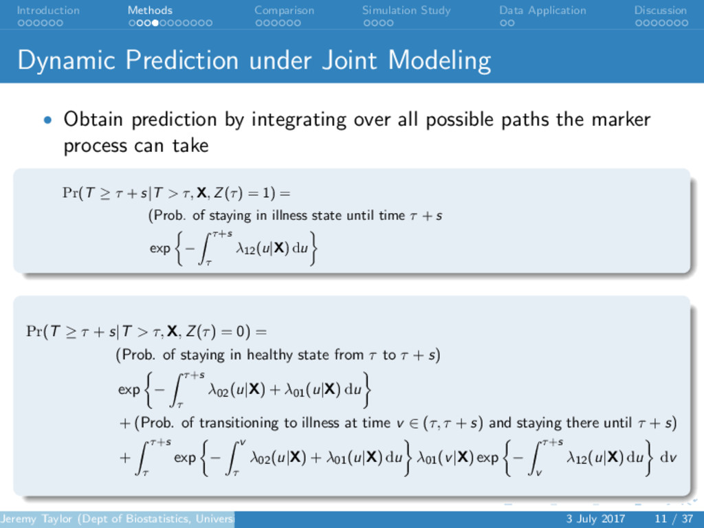
. . . . . . . . . . . . . . . . . . . . . . . . . . . . . . Introduction Methods Comparison Simulation Study Data Application Discussion Dynamic Prediction under Joint Modeling • Obtain prediction by integrating over all possible paths the marker process can take Pr(T ≥ τ + s|T > τ, X, Z(τ) = 1) = (Prob. of staying in illness state until time τ + s exp { − ∫ τ+s τ λ12(u|X) du } Pr(T ≥ τ + s|T > τ, X, Z(τ) = 0) = (Prob. of staying in healthy state from τ to τ + s) exp { − ∫ τ+s τ λ02(u|X) + λ01(u|X) du } + (Prob. of transitioning to illness at time v ∈ (τ, τ + s) and staying there until τ + s) + ∫ τ+s τ exp { − ∫ v τ λ02(u|X) + λ01(u|X) du } λ01(v|X) exp { − ∫ τ+s v λ12(u|X) du } dv Jeremy Taylor (Dept of Biostatistics, University of Michigan) 3 July 2017 11 / 37
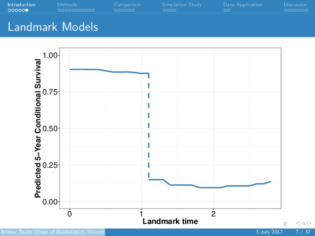
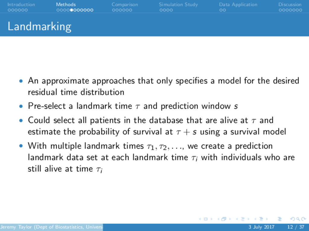
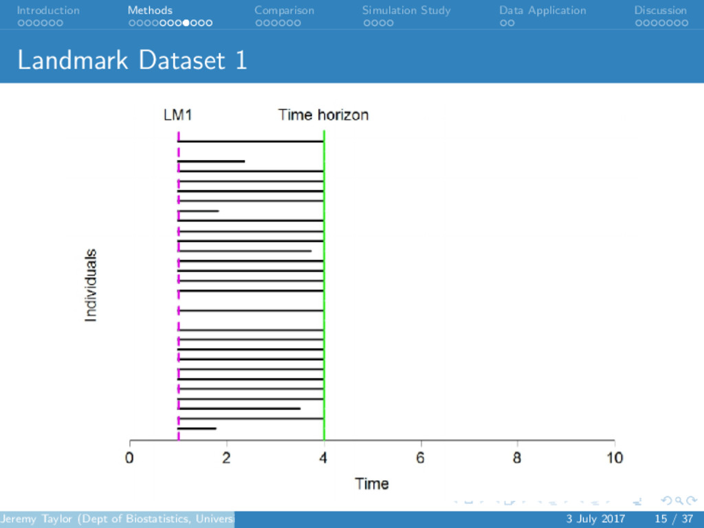
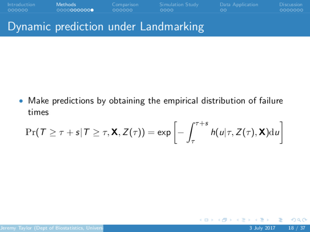
. . . . . . . . . . . . . . . . . . . . . . . . . . . . . . Introduction Methods Comparison Simulation Study Data Application Discussion Landmarking • An approximate approaches that only specifies a model for the desired residual time distribution • Pre-select a landmark time τ and prediction window s • Could select all patients in the database that are alive at τ and estimate the probability of survival at τ + s using a survival model • With multiple landmark times τ1, τ2, . . ., we create a prediction landmark data set at each landmark time τi with individuals who are still alive at time τi Jeremy Taylor (Dept of Biostatistics, University of Michigan) 3 July 2017 12 / 37
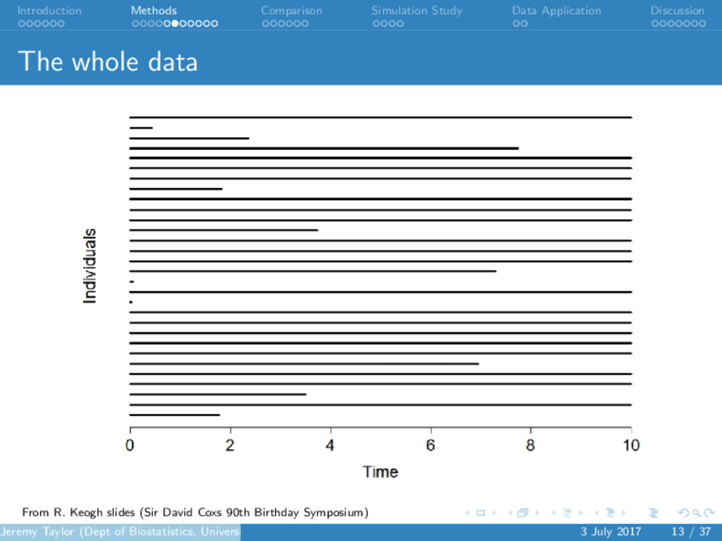
. . . . . . . . . . . . . . . . . . . . . . . . . . . . . . Introduction Methods Comparison Simulation Study Data Application Discussion The whole data From R. Keogh slides (Sir David Coxs 90th Birthday Symposium) Jeremy Taylor (Dept of Biostatistics, University of Michigan) 3 July 2017 13 / 37
. . . . . . . . . . . . . . . . . . . . . . . . . . . . . . Introduction Methods Comparison Simulation Study Data Application Discussion Landmark time 1 for the whole data Images from R. Keogh slides (Sir David Cox’s 90th Birthday Symposium) Jeremy Taylor (Dept of Biostatistics, University of Michigan) 3 July 2017 14 / 37
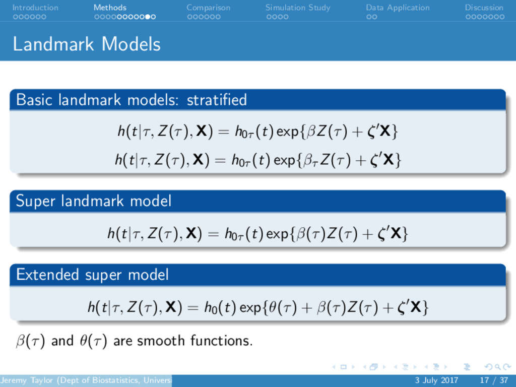
. . . . . . . . . . . . . . . . . . . . . . . . . . . . . . Introduction Methods Comparison Simulation Study Data Application Discussion Landmark Models • Create a data set for each landmark time τi with patients who are still alive at time τi and administrative censoring at time τi + s • Landmark data sets are stacked to create a “super data set” • Every subject must have a value of Z at each landmark time, may require imputation of Z • Last Observation Carried Forward • A longitudinal model for Z • A local average Jeremy Taylor (Dept of Biostatistics, University of Michigan) 3 July 2017 16 / 37
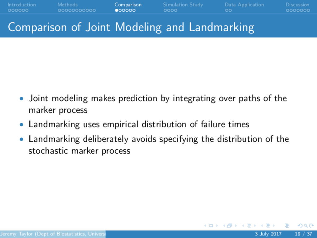
. . . . . . . . . . . . . . . . . . . . . . . . . . . . . . Introduction Methods Comparison Simulation Study Data Application Discussion Comparison of Joint Modeling and Landmarking • Joint modeling makes prediction by integrating over paths of the marker process • Landmarking uses empirical distribution of failure times • Landmarking deliberately avoids specifying the distribution of the stochastic marker process Jeremy Taylor (Dept of Biostatistics, University of Michigan) 3 July 2017 19 / 37
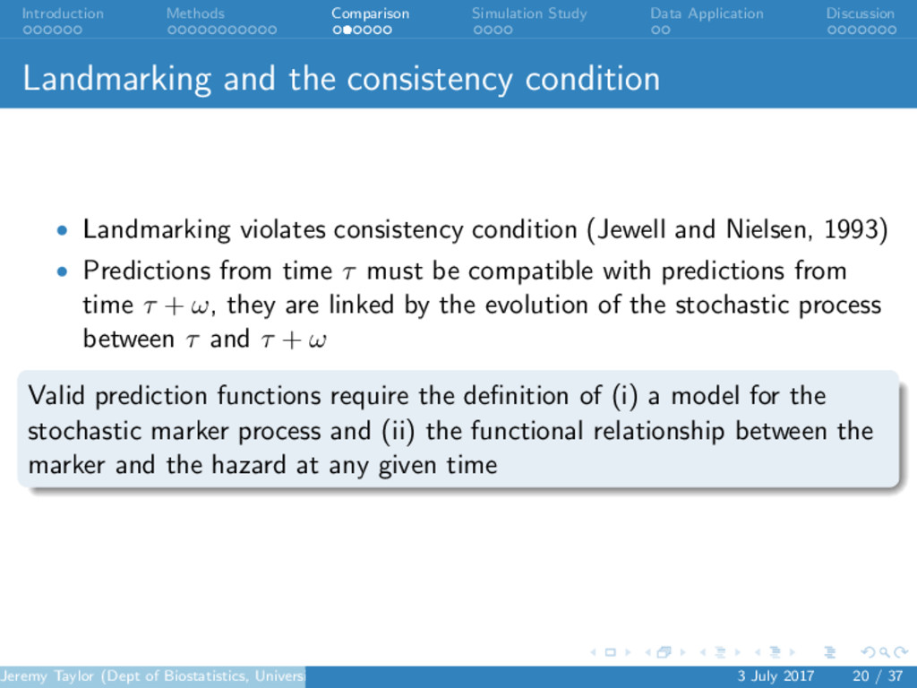
. . . . . . . . . . . . . . . . . . . . . . . . . . . . . . Introduction Methods Comparison Simulation Study Data Application Discussion Landmarking and the consistency condition • Landmarking violates consistency condition (Jewell and Nielsen, 1993) • Predictions from time τ must be compatible with predictions from time τ + ω, they are linked by the evolution of the stochastic process between τ and τ + ω Valid prediction functions require the definition of (i) a model for the stochastic marker process and (ii) the functional relationship between the marker and the hazard at any given time Jeremy Taylor (Dept of Biostatistics, University of Michigan) 3 July 2017 20 / 37
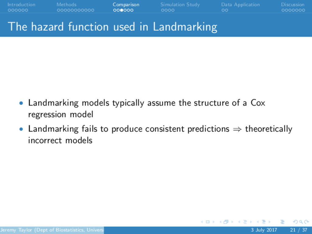
. . . . . . . . . . . . . . . . . . . . . . . . . . . . . . Introduction Methods Comparison Simulation Study Data Application Discussion The hazard function used in Landmarking • • Landmarking models typically assume the structure of a Cox regression model • Landmarking fails to produce consistent predictions ⇒ theoretically incorrect models Jeremy Taylor (Dept of Biostatistics, University of Michigan) 3 July 2017 21 / 37
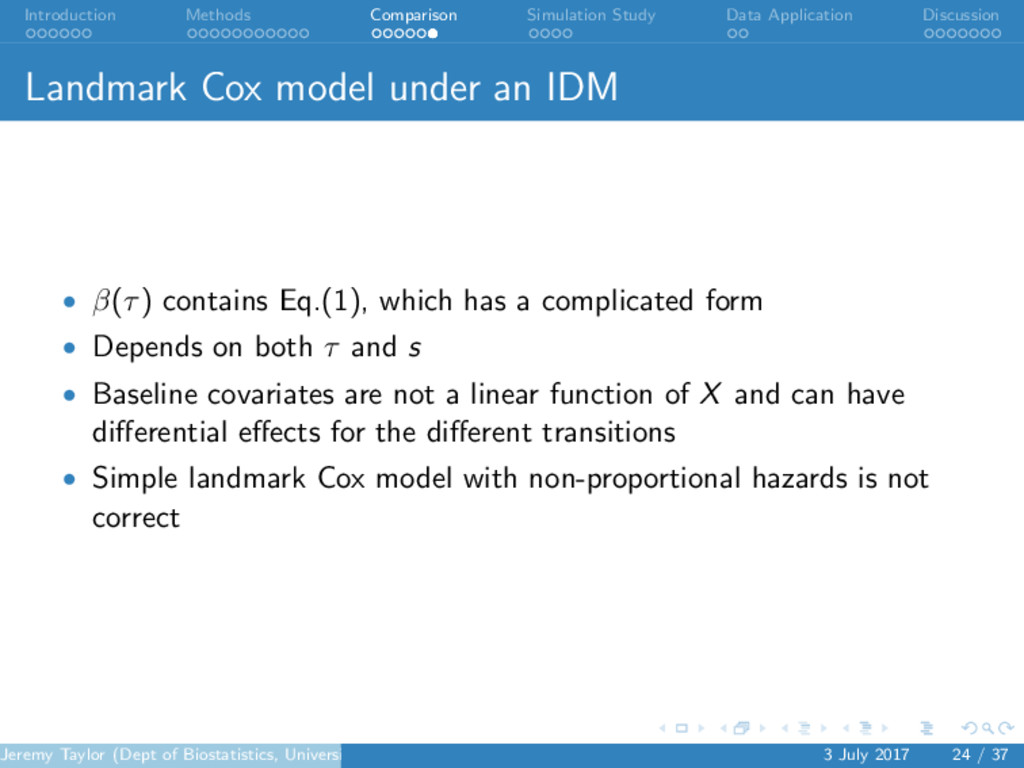
. . . . . . . . . . . . . . . . . . . . . . . . . . . . . . Introduction Methods Comparison Simulation Study Data Application Discussion Landmark Cox model under an IDM • β(τ) contains Eq.(1), which has a complicated form • Depends on both τ and s • Baseline covariates are not a linear function of X and can have differential effects for the different transitions • Simple landmark Cox model with non-proportional hazards is not correct Jeremy Taylor (Dept of Biostatistics, University of Michigan) 3 July 2017 24 / 37
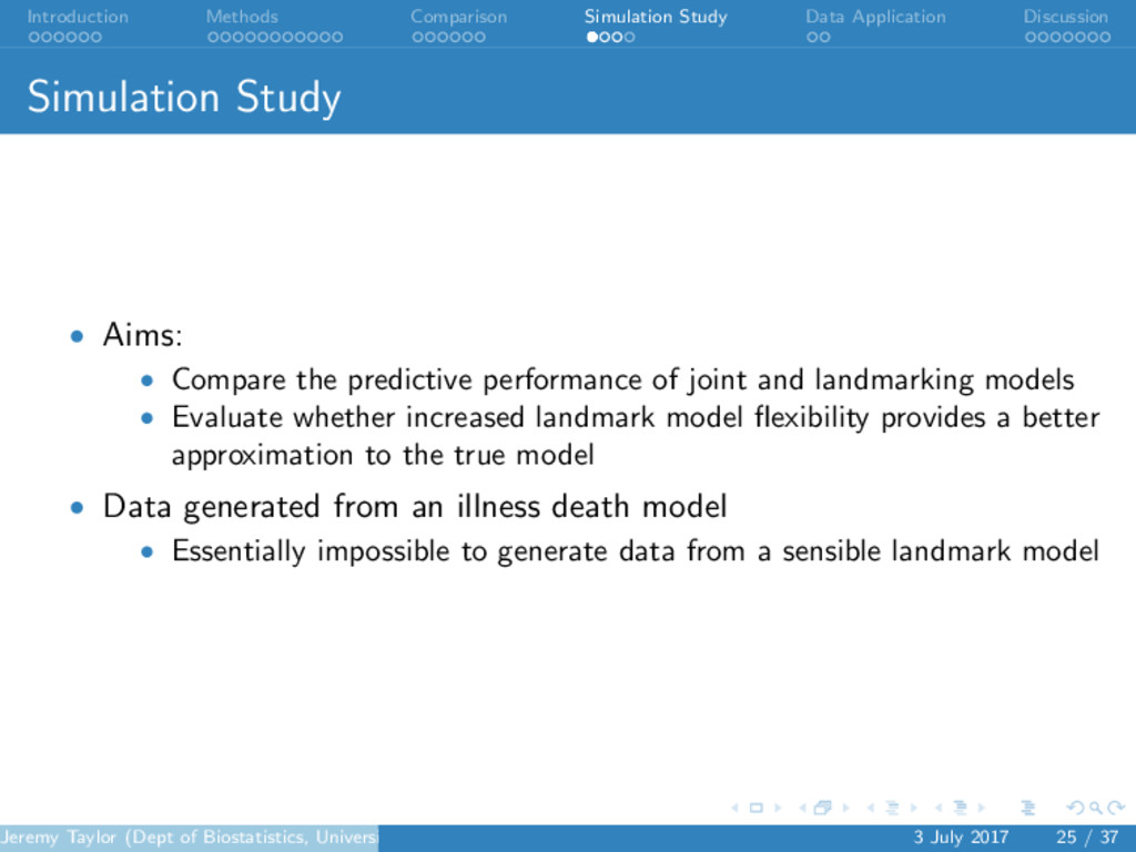
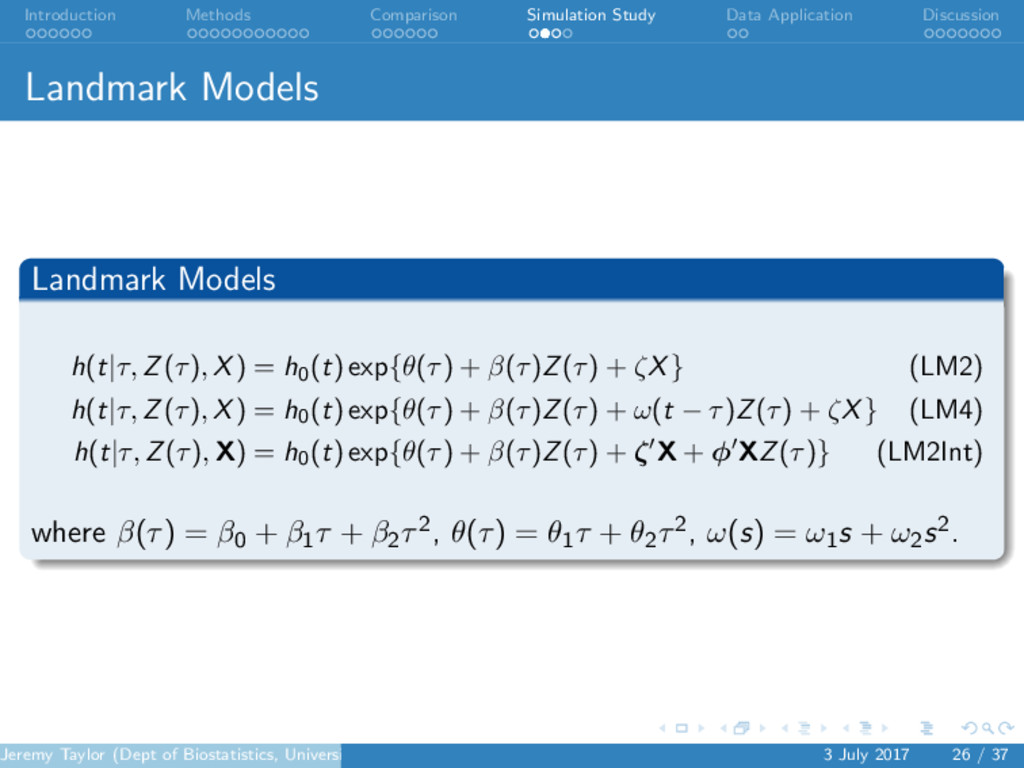
. . . . . . . . . . . . . . . . . . . . . . . . . . . . . . Introduction Methods Comparison Simulation Study Data Application Discussion Simulation Study • Aims: • Compare the predictive performance of joint and landmarking models • Evaluate whether increased landmark model flexibility provides a better approximation to the true model • Data generated from an illness death model • Essentially impossible to generate data from a sensible landmark model Jeremy Taylor (Dept of Biostatistics, University of Michigan) 3 July 2017 25 / 37
. . . . . . . . . . . . . . . . . . . . . . . . . . . . . . Introduction Methods Comparison Simulation Study Data Application Discussion Summary of Simulation Results • Joint modeling performs better than landmarking • Differences in Variance, AUC and R2 can be quite small • Absolute bias can be quite high for landmark model • Simple stratified landmark models usually perform similarly to those that were extended to allow different time scales • Interactions between baseline covariates and marker process improve landmark model approximation Jeremy Taylor (Dept of Biostatistics, University of Michigan) 3 July 2017 28 / 37
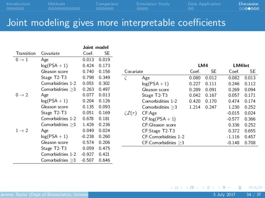
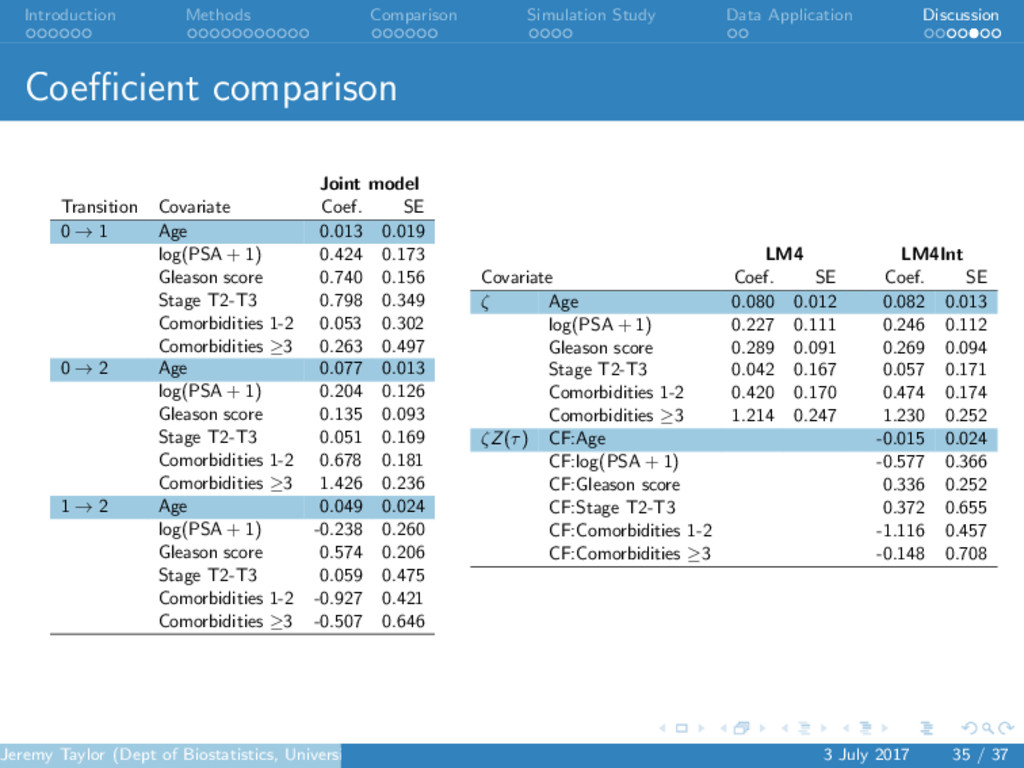
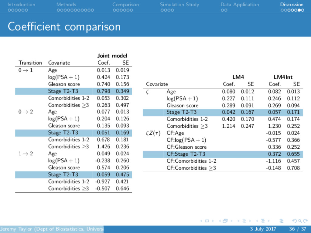
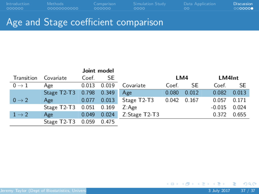
. . . . . . . . . . . . . . . . . . . . . . . . . . . . . . Introduction Methods Comparison Simulation Study Data Application Discussion Prostate cancer study • Prostate cancer study conducted at the University of Michigan • 745 patients with clinically localized prostate cancer treated with radiation therapy • Goal: Produce dynamic predictions of risk of death within 5 years • Measure time from start of treatment • Metastatic clinical failure (CF) is our time-dependent binary covariate (continuously observed) • Pretreatment prognostic factors: age, log-transformed PSA, Gleason score, prostate cancer stage, and comorbidities • Landmark times τ = 0, 1, . . . , 8 years Jeremy Taylor (Dept of Biostatistics, University of Michigan) 3 July 2017 29 / 37
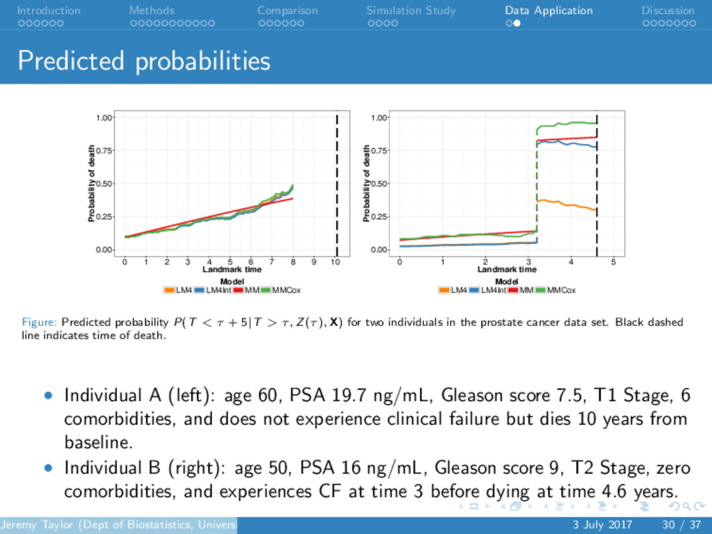
. . . . . . . . . . . . . . . . . . . . . . . . . . . . . . Introduction Methods Comparison Simulation Study Data Application Discussion Predicted probabilities 0.00 0.25 0.50 0.75 1.00 0 1 2 3 4 5 6 7 8 9 10 Landmark time Probability of death Model LM4 LM4Int MM MMCox 0.00 0.25 0.50 0.75 1.00 0 1 2 3 4 5 Landmark time Probability of death Model LM4 LM4Int MM MMCox Figure: Predicted probability P(T < τ + 5|T > τ, Z(τ), X) for two individuals in the prostate cancer data set. Black dashed line indicates time of death. • Individual A (left): age 60, PSA 19.7 ng/mL, Gleason score 7.5, T1 Stage, 6 comorbidities, and does not experience clinical failure but dies 10 years from baseline. • Individual B (right): age 50, PSA 16 ng/mL, Gleason score 9, T2 Stage, zero comorbidities, and experiences CF at time 3 before dying at time 4.6 years. Jeremy Taylor (Dept of Biostatistics, University of Michigan) 3 July 2017 30 / 37
. . . . . . . . . . . . . . . . . . . . . . . . . . . . . . Introduction Methods Comparison Simulation Study Data Application Discussion Discussion • Landmarking violates Jewell and Nielsen consistency criteria but can have similar predictive performance to joint modeling • Lots of modeling assumptions are needed for both joint modeling and landmarking • Joint modeling provides unified and principled approach • In situations where the marker process is well characterized or can be well estimated from the data, JM is likely to perform better and for longer prediction windows • Landmarking may provide a good approximation in situations with sparse longitudinal data and many longitudinal variables Jeremy Taylor (Dept of Biostatistics, University of Michigan) 3 July 2017 31 / 37