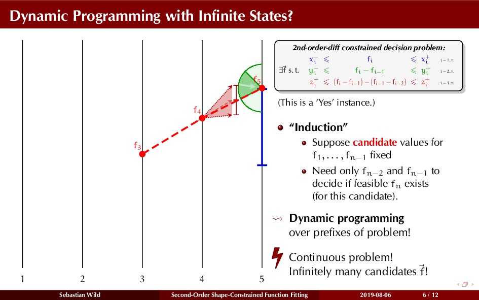
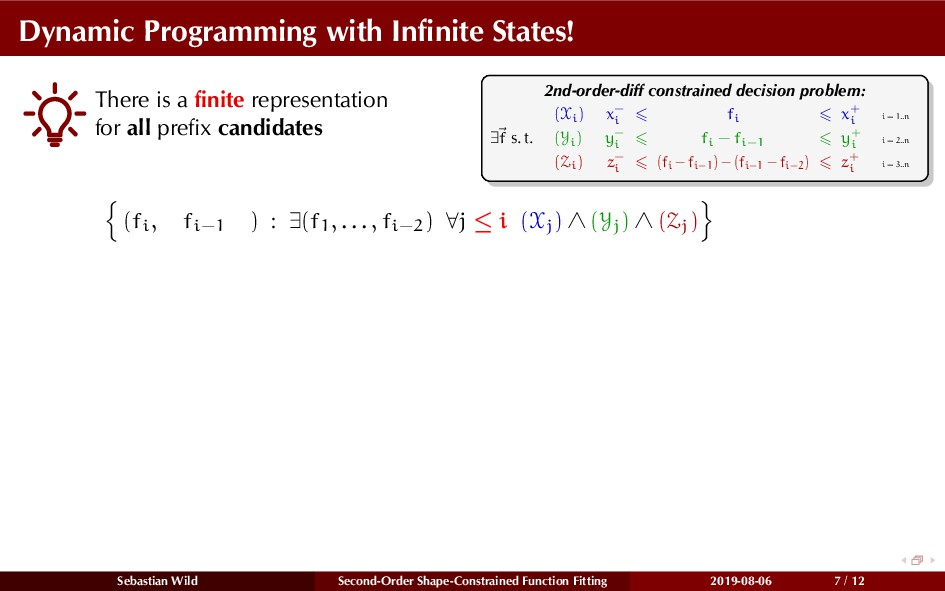
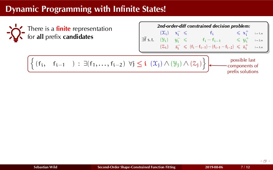
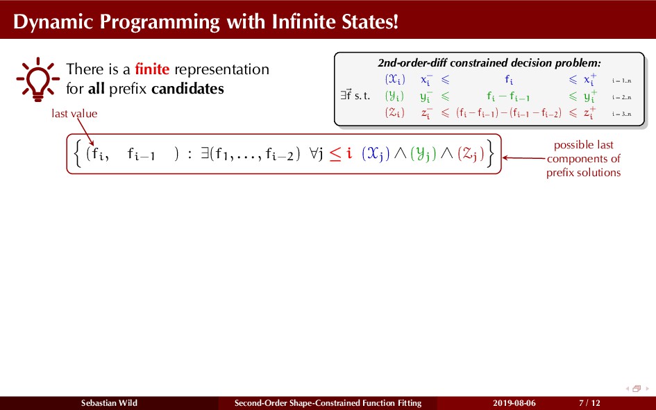
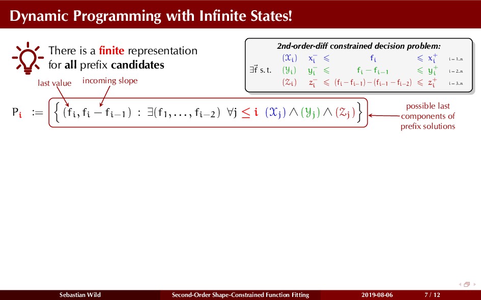
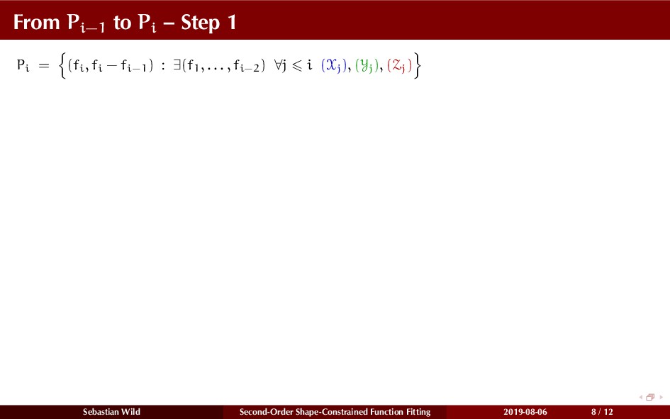
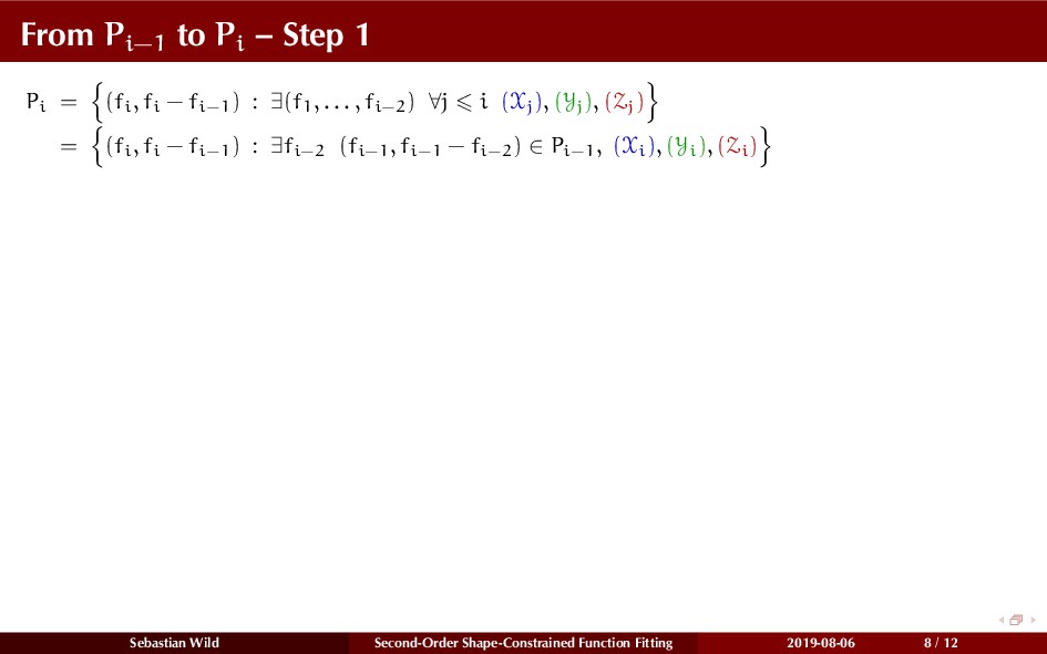
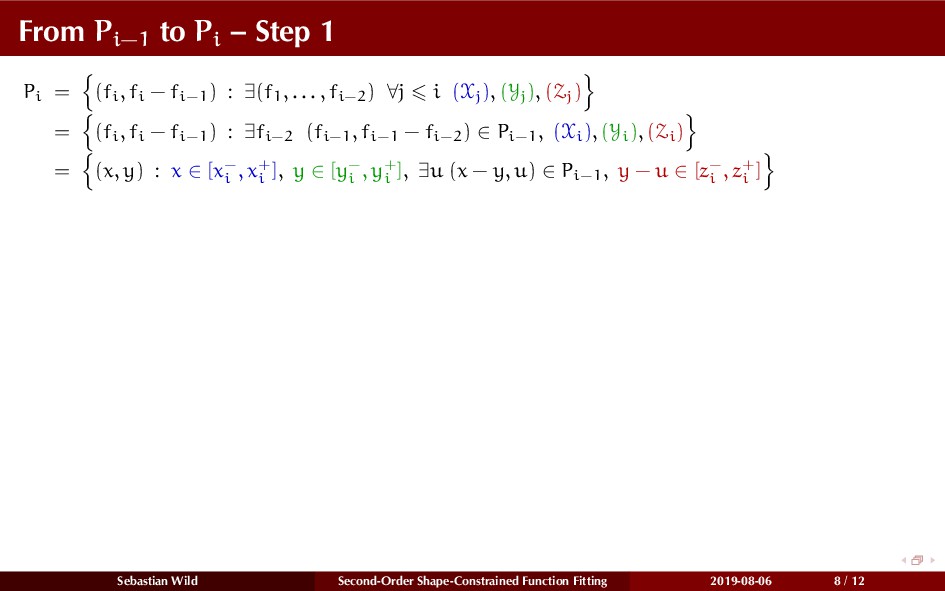
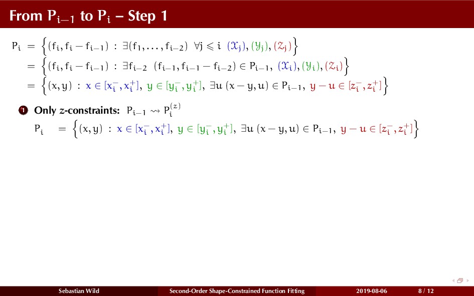
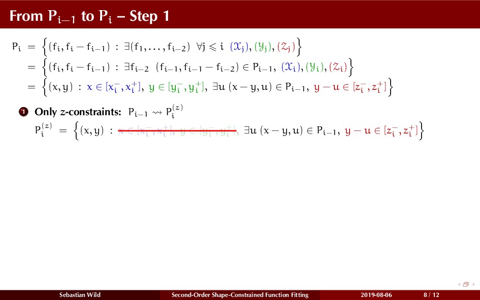
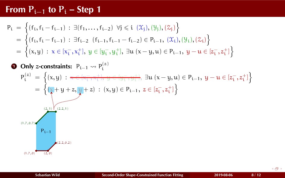
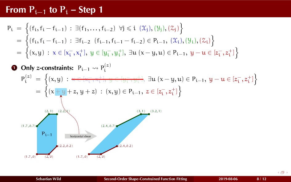
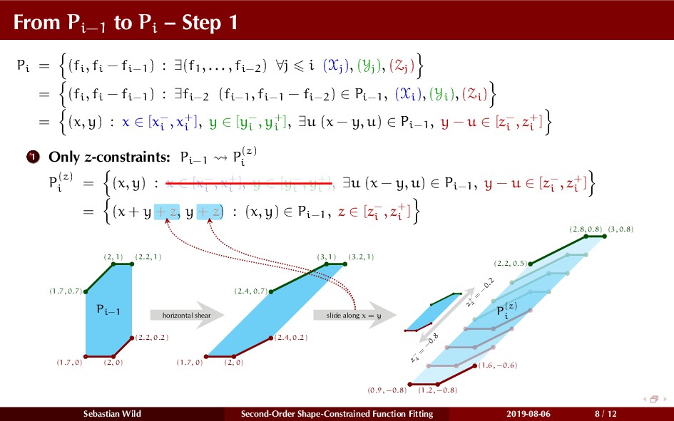
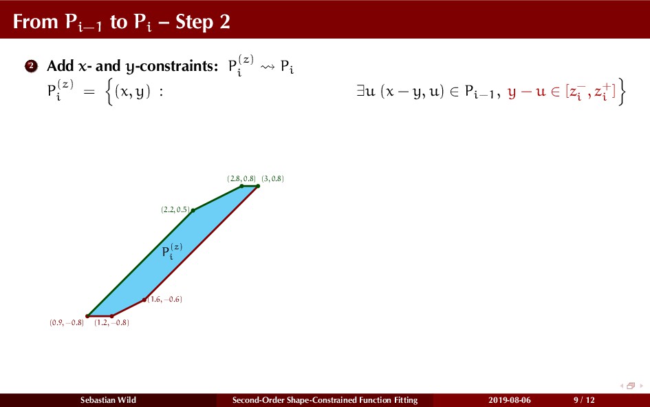
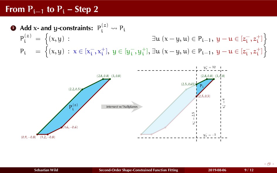
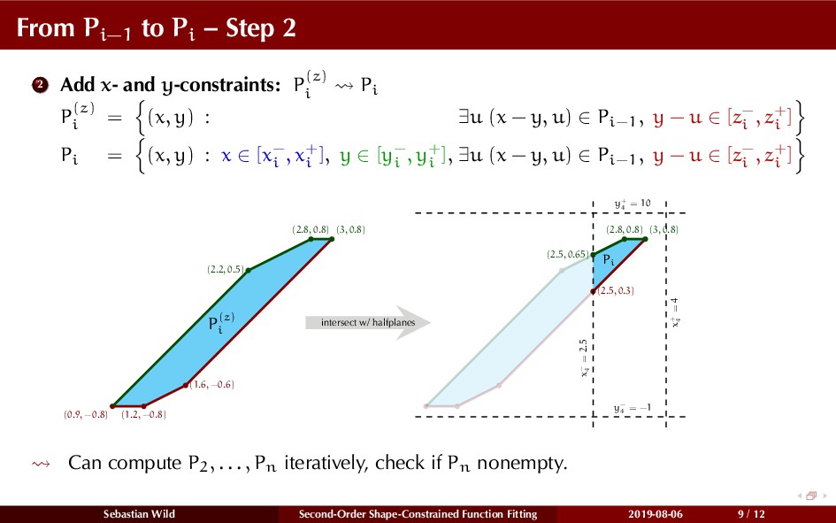
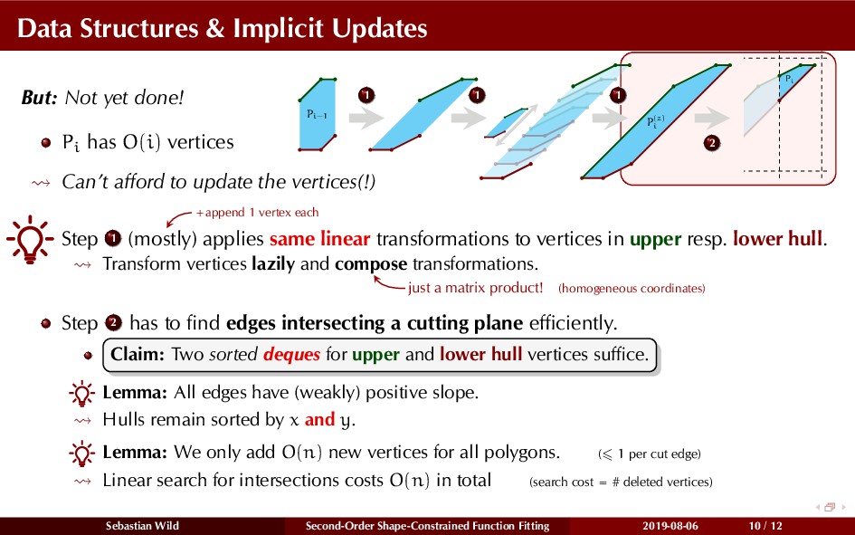
, fi − fi−1 ) : ∃(f1 , . . . , fi−2 ) ∀j i (Xj ), (Yj ), (Zj ) = (fi , fi − fi−1 ) : ∃fi−2 (fi−1 , fi−1 − fi−2 ) ∈ Pi−1 , (Xi ), (Yi ), (Zi ) = (x, y) : x ∈ [x− i , x+ i ], y ∈ [y− i , y+ i ], ∃u (x − y, u) ∈ Pi−1 , y − u ∈ [z− i , z+ i ] 1 Only z-constraints: Pi−1 P(z) i P(z) i = (x, y) : x ∈ [x− i , x+ i ], y ∈ [y− i , y+ i ], ∃u (x − y, u) ∈ Pi−1 , y − u ∈ [z− i , z+ i ] = (x + y + z, y + z) : (x, y) ∈ Pi−1 , z ∈ [z− i , z+ i ] (1.7, 0) (2, 0) (2.2, 0.2) (2.2, 1) (2, 1) (1.7, 0.7) Pi−1 horizontal shear (1.7, 0) (2, 0) (2.4, 0.2) (3.2, 1) (3, 1) (2.4, 0.7) slide along x = y + z + z z − 4 = − 0.8 z + 4 = − 0.2 (0.9, −0.8) (1.2, −0.8) (1.6, −0.6) (3, 0.8) (2.8, 0.8) (2.2, 0.5) P(z) i Sebastian Wild Second-Order Shape-Constrained Function Fitting 2019-08-06 8 / 12