Hypersuccinct Trees

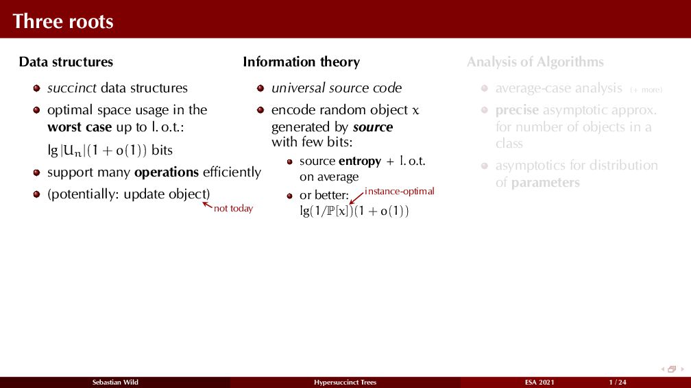
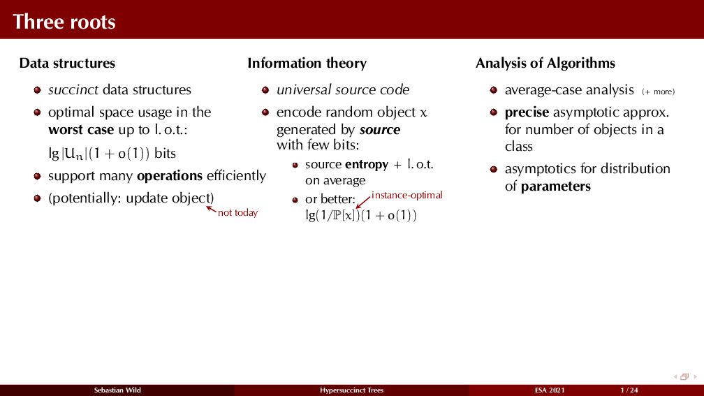
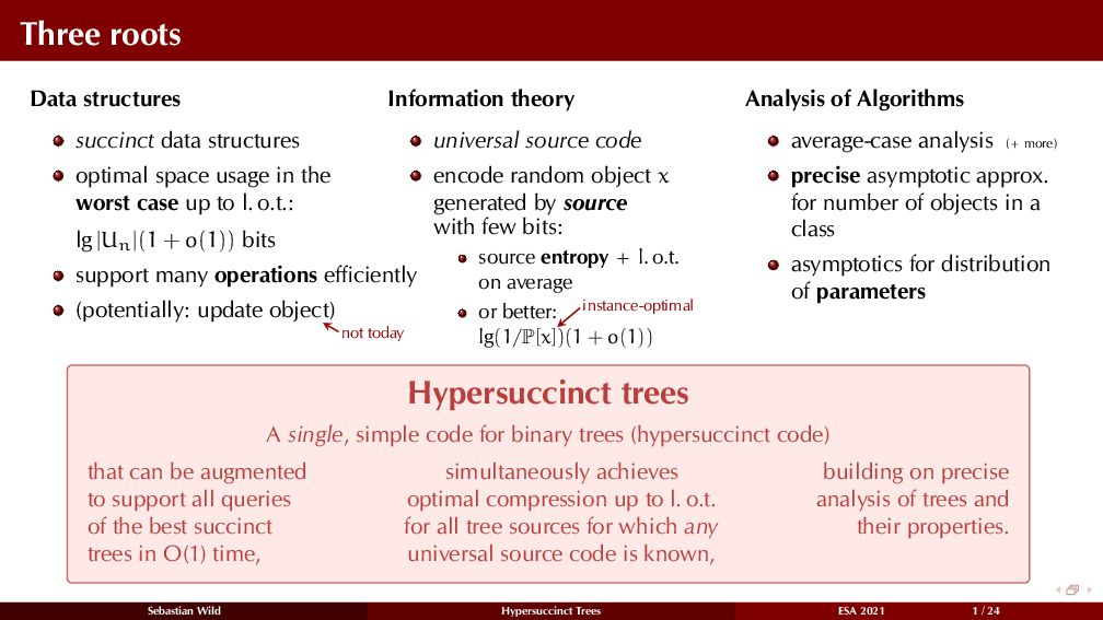
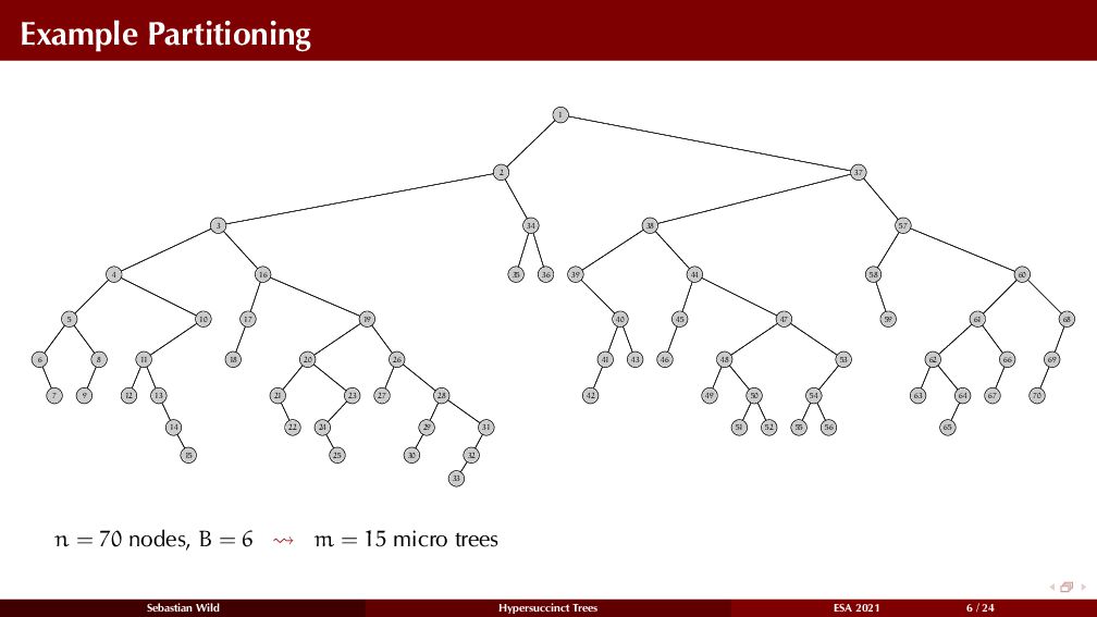
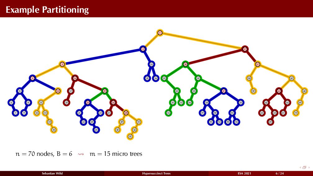
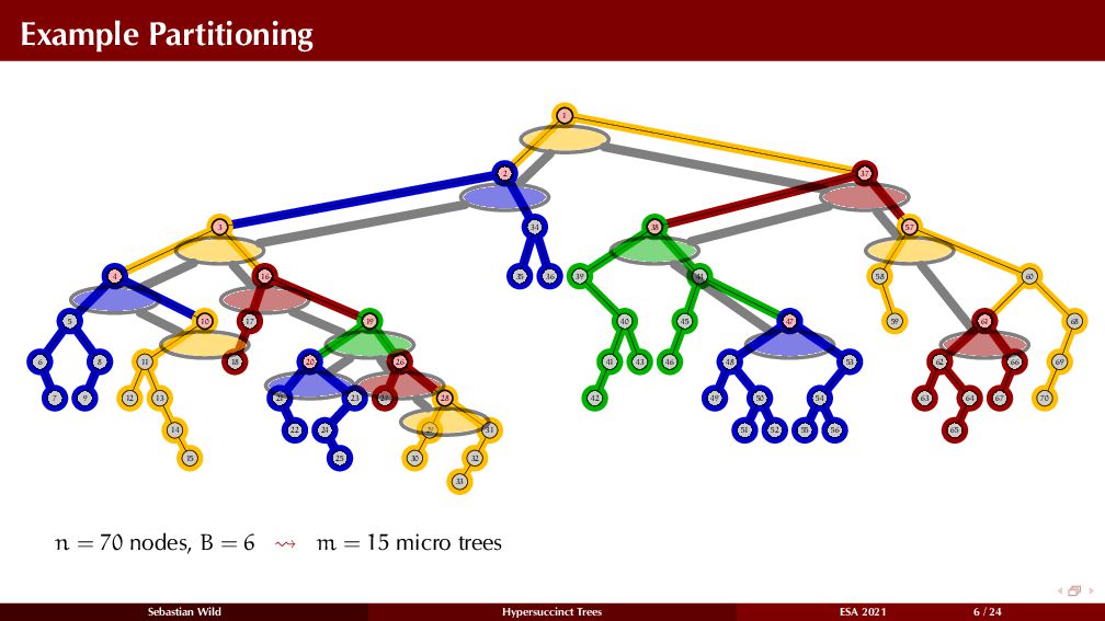
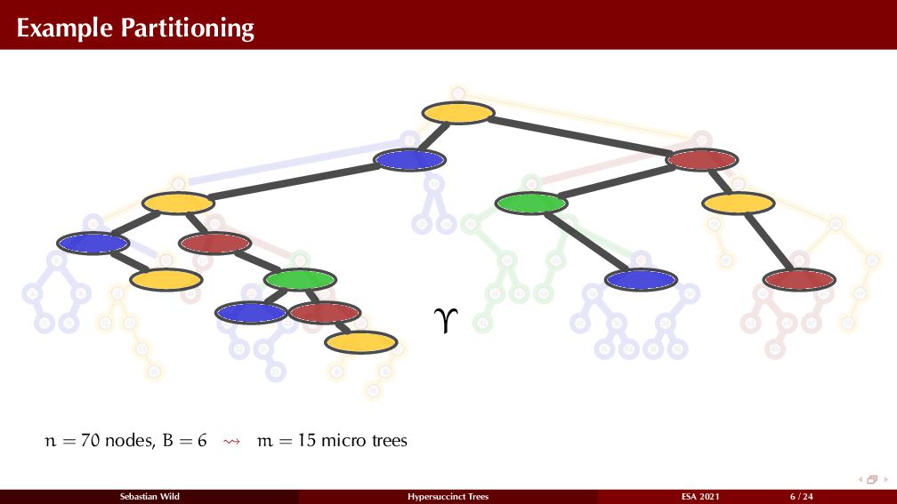
Slides from my presentation of our ESA 2021 paper on space-efficient tree data structures “Hypersuccinct Trees – New universal tree source codes for optimal compressed tree data structures and range minima”

The paper and further information can be found on the paper site:
https://www.wild-inter.net/publications/munro-nicholson-seelbach-benkner-wild-2021

Transcript

1. Hypersuccinct Trees New universal tree source codes for optimal compressed tree data structures and range minima Sebastian Wild joint work with Ian Munro, Pat Nicholson, and Louisa Seelbach Benkner arxiv.org/abs/2104.13457 European Symposium on Algorithms 2021 Sebastian Wild Hypersuccinct Trees ESA 2021 0 / 24
2. Outline 1 Three Roots 1 Three Roots 2 Hypersuccinct Trees 2 Hypersuccinct Trees 3 Tree Sources 3 Tree Sources 4 Two Favorite Trees 4 Two Favorite Trees 5 Range-Minimum Queries 5 Range-Minimum Queries Sebastian Wild Hypersuccinct Trees ESA 2021 0 / 24
3. 1 Three Roots 1 Three Roots Sebastian Wild Hypersuccinct Trees ESA 2021 0 / 24
4. Three roots Data structures succinct data structures optimal space usage in the worst case up to l. o.t.: lg |Un|(1 + o(1)) bits support many operations efficiently (potentially: update object) not today Information theory universal source code encode random object x generated by source with few bits: source entropy + l. o.t. on average or better: lg(1/P[x]) instance-optimal (1 + o(1)) Analysis of Algorithms average-case analysis (+ more) precise asymptotic approx. for number of objects in a class asymptotics for distribution of parameters Sebastian Wild Hypersuccinct Trees ESA 2021 1 / 24
5. Three roots Data structures succinct data structures optimal space usage in the worst case up to l. o.t.: lg |Un|(1 + o(1)) bits support many operations efficiently (potentially: update object) not today Information theory universal source code encode random object x generated by source with few bits: source entropy + l. o.t. on average or better: lg(1/P[x]) instance-optimal (1 + o(1)) Analysis of Algorithms average-case analysis (+ more) precise asymptotic approx. for number of objects in a class asymptotics for distribution of parameters Sebastian Wild Hypersuccinct Trees ESA 2021 1 / 24
6. Three roots Data structures succinct data structures optimal space usage in the worst case up to l. o.t.: lg |Un|(1 + o(1)) bits support many operations efficiently (potentially: update object) not today Information theory universal source code encode random object x generated by source with few bits: source entropy + l. o.t. on average or better: lg(1/P[x]) instance-optimal (1 + o(1)) Analysis of Algorithms average-case analysis (+ more) precise asymptotic approx. for number of objects in a class asymptotics for distribution of parameters Sebastian Wild Hypersuccinct Trees ESA 2021 1 / 24
7. Three roots Data structures succinct data structures optimal space usage in the worst case up to l. o.t.: lg |Un|(1 + o(1)) bits support many operations efficiently (potentially: update object) not today Information theory universal source code encode random object x generated by source with few bits: source entropy + l. o.t. on average or better: lg(1/P[x]) instance-optimal (1 + o(1)) Analysis of Algorithms average-case analysis (+ more) precise asymptotic approx. for number of objects in a class asymptotics for distribution of parameters Hypersuccinct trees A single, simple code for binary trees (hypersuccinct code) that can be augmented to support all queries of the best succinct trees in O(1) time, simultaneously achieves optimal compression up to l. o.t. for all tree sources for which any universal source code is known, building on precise analysis of trees and their properties. Sebastian Wild Hypersuccinct Trees ESA 2021 1 / 24
8. Outline 1 Three Roots 1 Three Roots 2 Hypersuccinct Trees 2 Hypersuccinct Trees 3 Tree Sources 3 Tree Sources 4 Two Favorite Trees 4 Two Favorite Trees 5 Range-Minimum Queries 5 Range-Minimum Queries Sebastian Wild Hypersuccinct Trees ESA 2021 1 / 24
9. 2 Hypersuccinct Trees 2 Hypersuccinct Trees Sebastian Wild Hypersuccinct Trees ESA 2021 1 / 24
10. Succinct Binary Trees What is known? data structure for ord a.k.a. plane trees inal or cardinal e.g. binary trees 2n + o(n) bits of space optimal in worst case some isolated works on better space for restricted scenarios but tailored approaches for each tree distribution supports huge list of operations in O(1) time on a standard word-RAM several competing approaches (BP, DFUDS, TC) (largely incompatible with each other) Operations in Tree Covering parent(v) the parent of v, same as anc(v, 1) degree(v) the number of children of v left_child(v) the left child of node v right_child(v) the right child of node v depth(v) the depth of v, i.e., the number of edges between the root and v anc(v, i) the ancestor of node v at depth depth(v) − i subtree_size(v) the number of descendants of v height(v) the height of the subtree rooted at node v LCA(v, u) the lowest common ancestor of nodes u and v leftmost_leaf(v) the leftmost leaf descendant of v rightmost_leaf(v) the rightmost leaf descendant of v level_leftmost(ℓ) the leftmost node on level ℓ level_rightmost(ℓ) the rightmost node on level ℓ level_predecessor(v) the node immediately to the left of v on the same level level_successor(v) the node immediately to the right of v on the same level node_rankX (v) the position of v in the X-order, X ∈ {PRE, POST, IN}, i.e., in a preorder, postorder, or inorder traversal node_selectX (i) the ith node in the X-order, X ∈ {PRE, POST, IN} leaf_rank(v) the number of leaves before and including v in pre- order leaf_select(i) the ith leaf in preorder Sebastian Wild Hypersuccinct Trees ESA 2021 2 / 24
11. Succinct Binary Trees What is known? data structure for ord a.k.a. plane trees inal or cardinal e.g. binary trees 2n + o(n) bits of space optimal in worst case some isolated works on better space for restricted scenarios but tailored approaches for each tree distribution supports huge list of operations in O(1) time on a standard word-RAM several competing approaches (BP, DFUDS, TC) (largely incompatible with each other) Operations in Tree Covering parent(v) the parent of v, same as anc(v, 1) degree(v) the number of children of v left_child(v) the left child of node v right_child(v) the right child of node v depth(v) the depth of v, i.e., the number of edges between the root and v anc(v, i) the ancestor of node v at depth depth(v) − i subtree_size(v) the number of descendants of v height(v) the height of the subtree rooted at node v LCA(v, u) the lowest common ancestor of nodes u and v leftmost_leaf(v) the leftmost leaf descendant of v rightmost_leaf(v) the rightmost leaf descendant of v level_leftmost(ℓ) the leftmost node on level ℓ level_rightmost(ℓ) the rightmost node on level ℓ level_predecessor(v) the node immediately to the left of v on the same level level_successor(v) the node immediately to the right of v on the same level node_rankX (v) the position of v in the X-order, X ∈ {PRE, POST, IN}, i.e., in a preorder, postorder, or inorder traversal node_selectX (i) the ith node in the X-order, X ∈ {PRE, POST, IN} leaf_rank(v) the number of leaves before and including v in pre- order leaf_select(i) the ith leaf in preorder Sebastian Wild Hypersuccinct Trees ESA 2021 2 / 24
12. Succinct Binary Trees What is known? data structure for ord a.k.a. plane trees inal or cardinal e.g. binary trees 2n + o(n) bits of space optimal in worst case some isolated works on better space for restricted scenarios but tailored approaches for each tree distribution supports huge list of operations in O(1) time on a standard word-RAM several competing approaches (BP, DFUDS, TC) (largely incompatible with each other) Operations in Tree Covering parent(v) the parent of v, same as anc(v, 1) degree(v) the number of children of v left_child(v) the left child of node v right_child(v) the right child of node v depth(v) the depth of v, i.e., the number of edges between the root and v anc(v, i) the ancestor of node v at depth depth(v) − i subtree_size(v) the number of descendants of v height(v) the height of the subtree rooted at node v LCA(v, u) the lowest common ancestor of nodes u and v leftmost_leaf(v) the leftmost leaf descendant of v rightmost_leaf(v) the rightmost leaf descendant of v level_leftmost(ℓ) the leftmost node on level ℓ level_rightmost(ℓ) the rightmost node on level ℓ level_predecessor(v) the node immediately to the left of v on the same level level_successor(v) the node immediately to the right of v on the same level node_rankX (v) the position of v in the X-order, X ∈ {PRE, POST, IN}, i.e., in a preorder, postorder, or inorder traversal node_selectX (i) the ith node in the X-order, X ∈ {PRE, POST, IN} leaf_rank(v) the number of leaves before and including v in pre- order leaf_select(i) the ith leaf in preorder Sebastian Wild Hypersuccinct Trees ESA 2021 2 / 24
13. Succinct Binary Trees What is known? data structure for ord a.k.a. plane trees inal or cardinal e.g. binary trees 2n + o(n) bits of space optimal in worst case some isolated works on better space for restricted scenarios but tailored approaches for each tree distribution supports huge list of operations in O(1) time on a standard word-RAM several competing approaches (BP, DFUDS, TC) (largely incompatible with each other) Operations in Tree Covering parent(v) the parent of v, same as anc(v, 1) degree(v) the number of children of v left_child(v) the left child of node v right_child(v) the right child of node v depth(v) the depth of v, i.e., the number of edges between the root and v anc(v, i) the ancestor of node v at depth depth(v) − i subtree_size(v) the number of descendants of v height(v) the height of the subtree rooted at node v LCA(v, u) the lowest common ancestor of nodes u and v leftmost_leaf(v) the leftmost leaf descendant of v rightmost_leaf(v) the rightmost leaf descendant of v level_leftmost(ℓ) the leftmost node on level ℓ level_rightmost(ℓ) the rightmost node on level ℓ level_predecessor(v) the node immediately to the left of v on the same level level_successor(v) the node immediately to the right of v on the same level node_rankX (v) the position of v in the X-order, X ∈ {PRE, POST, IN}, i.e., in a preorder, postorder, or inorder traversal node_selectX (i) the ith node in the X-order, X ∈ {PRE, POST, IN} leaf_rank(v) the number of leaves before and including v in pre- order leaf_select(i) the ith leaf in preorder Sebastian Wild Hypersuccinct Trees ESA 2021 2 / 24
14. Tree-Covering Data Structures Key idea: decompose tree into mini trees and mini trees into micro trees within o(n) space: can store ˜ O(log n) bits per mini tree enough to support many most comprehensive of all succinct trees operations and ˜ O(log log n) bits per micro tree only O( √ n) different micro tree shapes can store micro-tree-local operations in global lookup table (“4 Russians technique”) Sebastian Wild Hypersuccinct Trees ESA 2021 3 / 24
15. Tree-Covering Data Structures Key idea: decompose tree into mini trees and mini trees into micro trees within o(n) space: can store ˜ O(log n) bits per mini tree enough to support many most comprehensive of all succinct trees operations and ˜ O(log log n) bits per micro tree only O( √ n) different micro tree shapes can store micro-tree-local operations in global lookup table (“4 Russians technique”) Sebastian Wild Hypersuccinct Trees ESA 2021 3 / 24
16. Tree-Covering Data Structures Key idea: decompose tree into mini trees and mini trees into micro trees within o(n) space: can store ˜ O(log n) bits per mini tree enough to support many most comprehensive of all succinct trees operations and ˜ O(log log n) bits per micro tree only O( √ n) different micro tree shapes can store micro-tree-local operations in global lookup table (“4 Russians technique”) Sebastian Wild Hypersuccinct Trees ESA 2021 3 / 24
17. Tree-Covering Data Structures Key idea: decompose tree into mini trees and mini trees into micro trees within o(n) space: can store ˜ O(log n) bits per mini tree enough to support many most comprehensive of all succinct trees operations and ˜ O(log log n) bits per micro tree only O( √ n) different micro tree shapes can store micro-tree-local operations in global lookup table (“4 Russians technique”) Sebastian Wild Hypersuccinct Trees ESA 2021 3 / 24
18. Tree-Covering Data Structures Key idea: decompose tree into mini trees and mini trees into micro trees within o(n) space: can store ˜ O(log n) bits per mini tree enough to support many most comprehensive of all succinct trees operations and ˜ O(log log n) bits per micro tree only O( √ n) different micro tree shapes can store micro-tree-local operations in global lookup table (“4 Russians technique”) Dominant space: shapes of all micro trees everything else only o(n) bits Sebastian Wild Hypersuccinct Trees ESA 2021 3 / 24
19. Hypersuccinct code Essence of tree covering data structure yields simple code for binary trees! Given a binary tree t with micro trees µ1 , . . . , µm . Hypersuccinct code H(t) stores 1 How micro trees connect (o(n) bits) 2 Huffman codes C(µi ) of all micro trees |H(t)| = m i=1 |C(µi )| + o(n) Sebastian Wild Hypersuccinct Trees ESA 2021 4 / 24
20. Hypersuccinct code Essence of tree covering data structure yields simple code for binary trees! Given a binary tree t with micro trees µ1 , . . . , µm . Hypersuccinct code H(t) stores 1 How micro trees connect (o(n) bits) 2 Huffman codes C(µi ) of all micro trees |H(t)| = m i=1 |C(µi )| + o(n) Sebastian Wild Hypersuccinct Trees ESA 2021 4 / 24
21. Hypersuccinct code Essence of tree covering data structure yields simple code for binary trees! Given a binary tree t with micro trees µ1 , . . . , µm . Hypersuccinct code H(t) stores 1 How micro trees connect (o(n) bits) 2 Huffman codes C(µi ) of all micro trees |H(t)| = m i=1 |C(µi )| + o(n) Sebastian Wild Hypersuccinct Trees ESA 2021 4 / 24
22. Hypersuccinct code Essence of tree covering data structure yields simple code for binary trees! Given a binary tree t with micro trees µ1 , . . . , µm . Hypersuccinct code H(t) stores 1 How micro trees connect (o(n) bits) A n and m (Elias gamma code) B balanced-parenthesis (BP) bitstring for Υ (2m bits). C Huffman code for µ1 , . . . , µm : list of codewords and corresponding trees (size + BP) D position of portals in micro trees (2 O(log log n)-bit integers per µi ) 2 Huffman codes C(µi ) of all micro trees |H(t)| = m i=1 |C(µi )| + o(n) Sebastian Wild Hypersuccinct Trees ESA 2021 4 / 24
23. Hypersuccinct code Essence of tree covering data structure yields simple code for binary trees! Given a binary tree t with micro trees µ1 , . . . , µm . Hypersuccinct code H(t) stores 1 How micro trees connect (o(n) bits) A n and m (Elias gamma code) B balanced-parenthesis (BP) bitstring for Υ (2m bits). C Huffman code for µ1 , . . . , µm : list of codewords and corresponding trees (size + BP) D position of portals in micro trees (2 O(log log n)-bit integers per µi ) 2 Huffman codes C(µi ) of all micro trees |H(t)| = m i=1 |C(µi )| + o(n) Sebastian Wild Hypersuccinct Trees ESA 2021 4 / 24
24. Hypersuccinct code Essence of tree covering data structure yields simple code for binary trees! Given a binary tree t with micro trees µ1 , . . . , µm . Hypersuccinct code H(t) stores 1 How micro trees connect (o(n) bits) A n and m (Elias gamma code) B balanced-parenthesis (BP) bitstring for Υ (2m bits). C Huffman code for µ1 , . . . , µm : list of codewords and corresponding trees (size + BP) D position of portals in micro trees (2 O(log log n)-bit integers per µi ) 2 Huffman codes C(µi ) of all micro trees |H(t)| = m i=1 |C(µi )| + o(n) Sebastian Wild Hypersuccinct Trees ESA 2021 4 / 24
25. Farzan-Munro Algorithm How to (best) decompose a binary tree? Sebastian Wild Hypersuccinct Trees ESA 2021 5 / 24
26. Farzan-Munro Algorithm How to (best) decompose a binary tree? Farzan-Munro Algorithm Recursively: components C1 , C2 for left and right child u1 and u2 light? C = {v} ∪ C1 ∪ C2 u1 and u2 heavy? C = {v}, C1 , C2 , all marked permanent u1 heavy and u2 light? C1 permanent? C = {v} ∪ C2 otherwise |C1 | < B C = {v} ∪ C1 ∪ C2 If |C| B, mark it as permanent. Return C. Definition: v is heavy ⇐⇒ subtree_size(v) B Sebastian Wild Hypersuccinct Trees ESA 2021 5 / 24
27. Farzan-Munro Algorithm How to (best) decompose a binary tree? Farzan-Munro Algorithm Recursively: components C1 , C2 for left and right child u1 and u2 light? C = {v} ∪ C1 ∪ C2 u1 and u2 heavy? C = {v}, C1 , C2 , all marked permanent u1 heavy and u2 light? C1 permanent? C = {v} ∪ C2 otherwise |C1 | < B C = {v} ∪ C1 ∪ C2 If |C| B, mark it as permanent. Return C. Definition: v is heavy ⇐⇒ subtree_size(v) B Sebastian Wild Hypersuccinct Trees ESA 2021 5 / 24
28. Farzan-Munro Algorithm How to (best) decompose a binary tree? Farzan-Munro Algorithm Recursively: components C1 , C2 for left and right child u1 and u2 light? C = {v} ∪ C1 ∪ C2 u1 and u2 heavy? C = {v}, C1 , C2 , all marked permanent u1 heavy and u2 light? C1 permanent? C = {v} ∪ C2 otherwise |C1 | < B C = {v} ∪ C1 ∪ C2 If |C| B, mark it as permanent. Return C. Definition: v is heavy ⇐⇒ subtree_size(v) B Sebastian Wild Hypersuccinct Trees ESA 2021 5 / 24
29. Example Partitioning 12 13 16 19 23 25 28 32 36 42 51 56 59 64 6 10 11 14 15 17 18 1 20 21 22 24 26 27 29 2 30 31 33 34 35 37 38 39 3 40 41 43 44 45 46 47 48 49 4 50 52 53 54 55 57 58 5 60 61 62 63 65 66 67 68 69 70 7 8 9 6 14 15 10 3 18 17 16 21 22 20 7 24 25 23 19 27 26 30 29 28 33 5 32 31 2 35 34 36 1 39 42 41 9 40 43 38 46 45 44 49 48 51 50 8 52 47 55 54 56 53 37 58 59 57 4 63 62 65 64 61 67 66 60 70 69 12 68 11 13 n = 70 nodes, B = 6 m = 15 micro trees Sebastian Wild Hypersuccinct Trees ESA 2021 6 / 24
30. Example Partitioning 12 13 16 19 23 25 28 32 36 42 51 56 59 64 6 10 11 14 15 17 18 1 20 21 22 24 26 27 29 2 30 31 33 34 35 37 38 39 3 40 41 43 44 45 46 47 48 49 4 50 52 53 54 55 57 58 5 60 61 62 63 65 66 67 68 69 70 7 8 9 6 14 15 10 3 18 17 16 21 22 20 7 24 25 23 19 27 26 30 29 28 33 5 32 31 2 35 34 36 1 39 42 41 9 40 43 38 46 45 44 49 48 51 50 8 52 47 55 54 56 53 37 58 59 57 4 63 62 65 64 61 67 66 60 70 69 12 68 11 13 n = 70 nodes, B = 6 m = 15 micro trees Sebastian Wild Hypersuccinct Trees ESA 2021 6 / 24
31. Example Partitioning 12 13 16 19 23 25 28 32 36 42 51 56 59 64 6 10 11 14 15 17 18 1 20 21 22 24 26 27 29 2 30 31 33 34 35 37 38 39 3 40 41 43 44 45 46 47 48 49 4 50 52 53 54 55 57 58 5 60 61 62 63 65 66 67 68 69 70 7 8 9 6 14 15 10 3 18 17 16 21 22 20 7 24 25 23 19 27 26 30 29 28 33 5 32 31 2 35 34 36 1 39 42 41 9 40 43 38 46 45 44 49 48 51 50 8 52 47 55 54 56 53 37 58 59 57 4 63 62 65 64 61 67 66 60 70 69 12 68 11 13 36 32 56 42 13 59 23 19 25 64 51 12 6 16 28 n = 70 nodes, B = 6 m = 15 micro trees Sebastian Wild Hypersuccinct Trees ESA 2021 6 / 24
32. Example Partitioning 12 13 16 19 23 25 28 32 36 42 51 56 59 64 6 10 11 14 15 17 18 1 20 21 22 24 26 27 29 2 30 31 33 34 35 37 38 39 3 40 41 43 44 45 46 47 48 49 4 50 52 53 54 55 57 58 5 60 61 62 63 65 66 67 68 69 70 7 8 9 6 14 15 10 3 18 17 16 21 22 20 7 24 25 23 19 27 26 30 29 28 33 5 32 31 2 35 34 36 1 39 42 41 9 40 43 38 46 45 44 49 48 51 50 8 52 47 55 54 56 53 37 58 59 57 4 63 62 65 64 61 67 66 60 70 69 12 68 11 13 36 32 56 42 13 59 23 19 25 64 51 12 6 16 28 Υ n = 70 nodes, B = 6 m = 15 micro trees Sebastian Wild Hypersuccinct Trees ESA 2021 6 / 24
33. Properties of Micro Trees Binary tree t on n nodes is decomposed into µ1 , . . . , µm a m = O(n/B) (few micro trees) b |µi| = O(B) (all small) c |µ1| + · · · + |µm| = n (partition vertices) d µi has 3 edges to outside (parent, left, right) e root of µi is heavy f µi fringe |µi| B 12 13 16 19 23 25 28 32 36 42 51 56 59 64 6 10 11 14 15 17 18 1 20 21 22 24 26 27 29 2 30 31 33 34 35 37 38 39 3 40 41 43 44 45 46 47 48 49 4 50 52 53 54 55 57 58 5 60 61 62 63 65 66 67 68 69 70 7 8 9 6 14 15 10 3 18 17 16 21 22 20 7 24 25 23 19 27 26 30 29 28 33 5 32 31 2 35 34 36 1 39 42 41 9 40 43 38 46 45 44 49 48 51 50 8 52 47 55 54 56 53 37 58 59 57 4 63 62 65 64 61 67 66 60 70 69 12 68 11 13 36 32 56 42 13 59 23 19 25 64 51 12 6 16 28 Sebastian Wild Hypersuccinct Trees ESA 2021 7 / 24
34. Outline 1 Three Roots 1 Three Roots 2 Hypersuccinct Trees 2 Hypersuccinct Trees 3 Tree Sources 3 Tree Sources 4 Two Favorite Trees 4 Two Favorite Trees 5 Range-Minimum Queries 5 Range-Minimum Queries Sebastian Wild Hypersuccinct Trees ESA 2021 7 / 24
35. 3 Tree Sources 3 Tree Sources Sebastian Wild Hypersuccinct Trees ESA 2021 7 / 24
36. Universal Codes Information theory Study family of sources (e.g., memoryless sources for text, Markov sources) within that family: try to find universal codes (e.g., Lempel-Ziv compression) matches entropy of source up to l. o.t. without knowing source widely applicable compression method (Often) (relatively) simple algorithms whose analysis isn’t. Sebastian Wild Hypersuccinct Trees ESA 2021 8 / 24
37. Universal Codes Information theory Study family of sources (e.g., memoryless sources for text, Markov sources) within that family: try to find universal codes (e.g., Lempel-Ziv compression) matches entropy of source up to l. o.t. without knowing source widely applicable compression method (Often) (relatively) simple algorithms whose analysis isn’t. Sebastian Wild Hypersuccinct Trees ESA 2021 8 / 24
38. Universal Codes Information theory Study family of sources (e.g., memoryless sources for text, Markov sources) within that family: try to find universal codes (e.g., Lempel-Ziv compression) matches entropy of source up to l. o.t. without knowing source widely applicable compression method (Often) (relatively) simple algorithms whose analysis isn’t. Sebastian Wild Hypersuccinct Trees ESA 2021 8 / 24
39. Binary Tree Sources (Binary) tree source S = prob. distribution over tree shapes with a filter, e.g., tree of size n PS [t] = probability that S emits t Studied sources: memoryless type process: P[t] = v∈t p(type(v)) type(v) ∈ , , , kth-order type process: type prob. depends on types of k ancestors fixed-size source: for target size n, draw subtree sizes of root from given distribution P[t] = v∈t p(subtree_size(v.left), subtree_size(v.right)) fixed-height source: same with height of tree uniform subclass source: uniform distribution over subclass of trees Sebastian Wild Hypersuccinct Trees ESA 2021 9 / 24
40. Binary Tree Sources (Binary) tree source S = prob. distribution over tree shapes with a filter, e.g., tree of size n PS [t] = probability that S emits t Studied sources: memoryless type process: P[t] = v∈t p(type(v)) type(v) ∈ , , , kth-order type process: type prob. depends on types of k ancestors fixed-size source: for target size n, draw subtree sizes of root from given distribution P[t] = v∈t p(subtree_size(v.left), subtree_size(v.right)) fixed-height source: same with height of tree uniform subclass source: uniform distribution over subclass of trees Sebastian Wild Hypersuccinct Trees ESA 2021 9 / 24
41. Binary Tree Sources (Binary) tree source S = prob. distribution over tree shapes with a filter, e.g., tree of size n PS [t] = probability that S emits t Studied sources: memoryless type process: P[t] = v∈t p(type(v)) type(v) ∈ , , , kth-order type process: type prob. depends on types of k ancestors fixed-size source: for target size n, draw subtree sizes of root from given distribution P[t] = v∈t p(subtree_size(v.left), subtree_size(v.right)) fixed-height source: same with height of tree uniform subclass source: uniform distribution over subclass of trees Sebastian Wild Hypersuccinct Trees ESA 2021 9 / 24
42. Binary Tree Sources (Binary) tree source S = prob. distribution over tree shapes with a filter, e.g., tree of size n PS [t] = probability that S emits t Studied sources: memoryless type process: P[t] = v∈t p(type(v)) type(v) ∈ , , , kth-order type process: type prob. depends on types of k ancestors fixed-size source: for target size n, draw subtree sizes of root from given distribution P[t] = v∈t p(subtree_size(v.left), subtree_size(v.right)) fixed-height source: same with height of tree uniform subclass source: uniform distribution over subclass of trees Sebastian Wild Hypersuccinct Trees ESA 2021 9 / 24
43. Binary Tree Sources (Binary) tree source S = prob. distribution over tree shapes with a filter, e.g., tree of size n PS [t] = probability that S emits t Studied sources: memoryless type process: P[t] = v∈t p(type(v)) type(v) ∈ , , , kth-order type process: type prob. depends on types of k ancestors fixed-size source: for target size n, draw subtree sizes of root from given distribution P[t] = v∈t p(subtree_size(v.left), subtree_size(v.right)) fixed-height source: same with height of tree uniform subclass source: uniform distribution over subclass of trees Sebastian Wild Hypersuccinct Trees ESA 2021 9 / 24
44. Binary Tree Sources (Binary) tree source S = prob. distribution over tree shapes with a filter, e.g., tree of size n PS [t] = probability that S emits t Studied sources: memoryless type process: P[t] = v∈t p(type(v)) type(v) ∈ , , , kth-order type process: type prob. depends on types of k ancestors fixed-size source: for target size n, draw subtree sizes of root from given distribution P[t] = v∈t p(subtree_size(v.left), subtree_size(v.right)) fixed-height source: same with height of tree uniform subclass source: uniform distribution over subclass of trees Sebastian Wild Hypersuccinct Trees ESA 2021 9 / 24
45. Binary Tree Sources (Binary) tree source S = prob. distribution over tree shapes with a filter, e.g., tree of size n PS [t] = probability that S emits t Studied sources: memoryless type process: P[t] = v∈t p(type(v)) type(v) ∈ , , , kth-order type process: type prob. depends on types of k ancestors fixed-size source: for target size n, draw subtree sizes of root from given distribution P[t] = v∈t p(subtree_size(v.left), subtree_size(v.right)) fixed-height source: same with height of tree uniform subclass source: uniform distribution over subclass of trees Universal codes can’t exist in full generality! can be different for every n! Sebastian Wild Hypersuccinct Trees ESA 2021 9 / 24
46. Tame Binary Tree Sources Family of sources Restriction Redundancy Memoryless node-type — O(n log log n/ log n) kth-order node-type — O((nk + n log log n)/ log n) Monotonic fixed-size p(ℓ, r) p(ℓ + 1, r) and p(ℓ, r) p(ℓ, r + 1) for all ℓ, r ∈ N0 O(n log log n/ log n) Worst-case fringe-dominated fixed-size n B (t) = o(n/ log log n) for all t with P[t] > 0; n B (t) = #nodes with subtree size in Ω(log n) O n B (t) log log n + n log log n/ log n Weight-balanced fixed-size n c ℓ n− n c p(ℓ − 1, n − ℓ − 1) = 1 for constant c 3 O(n log log n/ log n) Average-case fringe-dominated fixed-size E[n B (T)] = o(n/ log log n) for random T generated by source S O n B (t) log log n + n log log n/ log n Monotonic fixed-height p(ℓ, r) p(ℓ + 1, r) and p(ℓ, r) p(ℓ, r + 1) for all ℓ, r ∈ N0 O(n log log n/ log n) Worst-case fringe-dominated fixed-height n B (t) = o(n/ log log n) for all t with P[t] > 0 O n B (t) log log n + n log log n/ log n Tame uniform-subclass class of trees Tn(P) is hereditary (i.e., closed under taking subtrees), n B (t) = o(n/ log log n) for t ∈ Tn(P), lg |Tn(P)| = cn + o(n) for constant c > 0, heavy-twigged: if v has subtree size Ω(log n), v’s subtrees have size ω(1) o(n) Sebastian Wild Hypersuccinct Trees ESA 2021 10 / 24
47. Optimally compressed binary tree distributions Tree-Shape Distribution Entropy Corresponding Source (Uniformly random) binary trees of size n 2n Memoryless binary, monotonic fixed-size binary (Uniformly random) full binary trees of size n n Memoryless binary (Uniformly random) unary paths of length n n Memoryless binary (Uniformly random) Motzkin trees of size n 1.585n Memoryless binary BSTs generated by insertions in random order 1.736n Monotonic fixed-size binary Binomial random trees P(lg n)n a) Average-case fringe-dominated fixed-size binary Almost paths — b) Monotonic fixed-size binary Random fringe-balanced binary search trees — b) Average-case fringe-dominated fixed-size binary (Uniformly random) AVL trees of height h — b) Worst-case fringe-dominated fixed-height binary (Uniformly random) weight-balanced binary trees of size n — b) Worst-case fringe-dominated fixed-size binary (Uniformly random) AVL trees of size n 0.938n Uniform-subclass (Uniformly random) left-leaning red-black trees of size n 0.879n Uniform-subclass a) Here P is a nonconstant, continuous, periodic function with period 1. b) No (concise) asymptotic approximation known. Sebastian Wild Hypersuccinct Trees ESA 2021 11 / 24
48. Outline 1 Three Roots 1 Three Roots 2 Hypersuccinct Trees 2 Hypersuccinct Trees 3 Tree Sources 3 Tree Sources 4 Two Favorite Trees 4 Two Favorite Trees 5 Range-Minimum Queries 5 Range-Minimum Queries Sebastian Wild Hypersuccinct Trees ESA 2021 11 / 24
49. 4 Two Favorite Trees 4 Two Favorite Trees Sebastian Wild Hypersuccinct Trees ESA 2021 11 / 24
50. Two Examples Here: two representative examples 1 Random BSTs Start with a random permutation π of {1, . . . , n} Successively insert π1 , . . . , πn into initially empty (unbalanced) BST. Challenge: highly non-uniform distribution 2 (uniform) Weight-Balanced BSTs (BB[α]) parameter α ∈ (0, 1 2 ) α-balanced = at every node v holds: subtree_size(v.left ) + 1 α(subtree_size(v) + 1) subtree_size(v.right) + 1 α(subtree_size(v) + 1) Challenge: support is small subclass; non-fringe µi might not be α-balanced ideas can be generalized to families of sources Sebastian Wild Hypersuccinct Trees ESA 2021 12 / 24
51. Two Examples Here: two representative examples 1 Random BSTs Start with a random permutation π of {1, . . . , n} Successively insert π1 , . . . , πn into initially empty (unbalanced) BST. Challenge: highly non-uniform distribution 2 (uniform) Weight-Balanced BSTs (BB[α]) parameter α ∈ (0, 1 2 ) α-balanced = at every node v holds: subtree_size(v.left ) + 1 α(subtree_size(v) + 1) subtree_size(v.right) + 1 α(subtree_size(v) + 1) Challenge: support is small subclass; non-fringe µi might not be α-balanced ideas can be generalized to families of sources Sebastian Wild Hypersuccinct Trees ESA 2021 12 / 24
52. Two Examples Here: two representative examples 1 Random BSTs Start with a random permutation π of {1, . . . , n} Successively insert π1 , . . . , πn into initially empty (unbalanced) BST. Challenge: highly non-uniform distribution 2 (uniform) Weight-Balanced BSTs (BB[α]) parameter α ∈ (0, 1 2 ) α-balanced = at every node v holds: subtree_size(v.left ) + 1 α(subtree_size(v) + 1) subtree_size(v.right) + 1 α(subtree_size(v) + 1) Challenge: support is small subclass; non-fringe µi might not be α-balanced ideas can be generalized to families of sources Sebastian Wild Hypersuccinct Trees ESA 2021 12 / 24
53. Two Examples Here: two representative examples 1 Random BSTs Start with a random permutation π of {1, . . . , n} Successively insert π1 , . . . , πn into initially empty (unbalanced) BST. Challenge: highly non-uniform distribution 2 (uniform) Weight-Balanced BSTs (BB[α]) parameter α ∈ (0, 1 2 ) α-balanced = at every node v holds: subtree_size(v.left ) + 1 α(subtree_size(v) + 1) subtree_size(v.right) + 1 α(subtree_size(v) + 1) Challenge: support is small subclass; non-fringe µi might not be α-balanced ideas can be generalized to families of sources Sebastian Wild Hypersuccinct Trees ESA 2021 12 / 24
54. Two Examples Here: two representative examples 1 Random BSTs Start with a random permutation π of {1, . . . , n} Successively insert π1 , . . . , πn into initially empty (unbalanced) BST. Challenge: highly non-uniform distribution 2 (uniform) Weight-Balanced BSTs (BB[α]) parameter α ∈ (0, 1 2 ) α-balanced = at every node v holds: subtree_size(v.left ) + 1 α(subtree_size(v) + 1) subtree_size(v.right) + 1 α(subtree_size(v) + 1) Challenge: support is small subclass; non-fringe µi might not be α-balanced ideas can be generalized to families of sources Sebastian Wild Hypersuccinct Trees ESA 2021 12 / 24
55. Random BSTs – Outline Random BSTs: rank of root uniform every possible split equally likely P[t] = v∈t 1 subtree_sizet (v) random BSTs = fixed-size source with p(ℓ, n − 1 − ℓ) = 1 n (n ∈ N 1 and ℓ ∈ {0, . . . , n − 1}) Step 1 Construct a source-specific micro-tree encoding DS : {µ1 , . . . , µm} → {0, 1}⋆ Goal: |DS (µi )| ≈ lg(1/P[µi ]) Step 2 By optimality of Huffman codes: m i=1 |C(µi )| m i=1 |DS (µi )| Step 3 Use properties of S to show that m i=1 P[µi ] P[t] Step 4 Conclude m i=1 |C(µi )| ≈ lg(1/P[t]) Sebastian Wild Hypersuccinct Trees ESA 2021 13 / 24
56. Random BSTs – Outline Random BSTs: rank of root uniform every possible split equally likely P[t] = v∈t 1 subtree_sizet (v) random BSTs = fixed-size source with p(ℓ, n − 1 − ℓ) = 1 n (n ∈ N 1 and ℓ ∈ {0, . . . , n − 1}) Step 1 Construct a source-specific micro-tree encoding DS : {µ1 , . . . , µm} → {0, 1}⋆ Goal: |DS (µi )| ≈ lg(1/P[µi ]) Step 2 By optimality of Huffman codes: m i=1 |C(µi )| m i=1 |DS (µi )| Step 3 Use properties of S to show that m i=1 P[µi ] P[t] Step 4 Conclude m i=1 |C(µi )| ≈ lg(1/P[t]) Sebastian Wild Hypersuccinct Trees ESA 2021 13 / 24
57. Random BSTs – Outline Random BSTs: rank of root uniform every possible split equally likely P[t] = v∈t 1 subtree_sizet (v) random BSTs = fixed-size source with p(ℓ, n − 1 − ℓ) = 1 n (n ∈ N 1 and ℓ ∈ {0, . . . , n − 1}) Step 1 Construct a source-specific micro-tree encoding DS : {µ1 , . . . , µm} → {0, 1}⋆ Goal: |DS (µi )| ≈ lg(1/P[µi ]) Step 2 By optimality of Huffman codes: m i=1 |C(µi )| m i=1 |DS (µi )| Step 3 Use properties of S to show that m i=1 P[µi ] P[t] Step 4 Conclude m i=1 |C(µi )| ≈ lg(1/P[t]) Sebastian Wild Hypersuccinct Trees ESA 2021 13 / 24
58. Random BSTs – Outline Random BSTs: rank of root uniform every possible split equally likely P[t] = v∈t 1 subtree_sizet (v) random BSTs = fixed-size source with p(ℓ, n − 1 − ℓ) = 1 n (n ∈ N 1 and ℓ ∈ {0, . . . , n − 1}) Step 1 Construct a source-specific micro-tree encoding DS : {µ1 , . . . , µm} → {0, 1}⋆ Goal: |DS (µi )| ≈ lg(1/P[µi ]) Step 2 By optimality of Huffman codes: m i=1 |C(µi )| m i=1 |DS (µi )| Step 3 Use properties of S to show that m i=1 P[µi ] P[t] Step 4 Conclude m i=1 |C(µi )| ≈ lg(1/P[t]) Sebastian Wild Hypersuccinct Trees ESA 2021 13 / 24
59. Random BSTs – Source-specific code Step 1 Code DS for µ1 , . . . , µm with |DS (µi )| ∼ lg(1/|PS [µi ]) 1 store |µi| Elias code 2 store left subtree sizes in depth-first traversal using arithmetic coding 2a Encode sequence of outcomes as subinterval I of [0, 1) = I0 Know subtree_size(v1 ) = |µi | = 5 (from 1 ) for v1 , left subtree size ℓ1 ∈ {0, 1, 2, 3, 4} identify with subintervals of I0 of lengths p(ℓ1 , 4 − ℓ1 )|I0 | = 1 5 here ℓ1 = 3 I1 = [3 5 , 4 5 ) know subtree_size(v2 ) = ℓ1 = 3 left subtree size ℓ2 ∈ {0, 1, 2} use subintervals of I1 of lengths p(ℓ1 , 2 − ℓ1 )|I1 | = 1 3 · 1 5 here ℓ2 = 1, I2 = [3 5 + 1 15 , 3 5 + 2 15 ) = [2 3 , 11 15 ) subtree_size(v3 ) = ℓ2 = 1, so ℓ3 = 0. nothing to store! v4 and v5 same I = [2 3 , 11 15 ) v1 v2 v3 v4 v5 2b Arithmetic coding: Find interval [ m 2l , m+1 2l ) ⊆ I (l, m ∈ N) Here: [22 32 , 23 32 ) encode I by l-bit binary representation of m. Here: 10110 Always have l lg(1/|I|) + 2 Sebastian Wild Hypersuccinct Trees ESA 2021 14 / 24
60. Random BSTs – Source-specific code Step 1 Code DS for µ1 , . . . , µm with |DS (µi )| ∼ lg(1/|PS [µi ]) 1 store |µi| Elias code 2 store left subtree sizes in depth-first traversal using arithmetic coding 2a Encode sequence of outcomes as subinterval I of [0, 1) = I0 Know subtree_size(v1 ) = |µi | = 5 (from 1 ) for v1 , left subtree size ℓ1 ∈ {0, 1, 2, 3, 4} identify with subintervals of I0 of lengths p(ℓ1 , 4 − ℓ1 )|I0 | = 1 5 here ℓ1 = 3 I1 = [3 5 , 4 5 ) know subtree_size(v2 ) = ℓ1 = 3 left subtree size ℓ2 ∈ {0, 1, 2} use subintervals of I1 of lengths p(ℓ1 , 2 − ℓ1 )|I1 | = 1 3 · 1 5 here ℓ2 = 1, I2 = [3 5 + 1 15 , 3 5 + 2 15 ) = [2 3 , 11 15 ) subtree_size(v3 ) = ℓ2 = 1, so ℓ3 = 0. nothing to store! v4 and v5 same I = [2 3 , 11 15 ) v1 v2 v3 v4 v5 2b Arithmetic coding: Find interval [ m 2l , m+1 2l ) ⊆ I (l, m ∈ N) Here: [22 32 , 23 32 ) encode I by l-bit binary representation of m. Here: 10110 Always have l lg(1/|I|) + 2 Sebastian Wild Hypersuccinct Trees ESA 2021 14 / 24
61. Random BSTs – Source-specific code Step 1 Code DS for µ1 , . . . , µm with |DS (µi )| ∼ lg(1/|PS [µi ]) 1 store |µi| Elias code 2 store left subtree sizes in depth-first traversal using arithmetic coding 2a Encode sequence of outcomes as subinterval I of [0, 1) = I0 Know subtree_size(v1 ) = |µi | = 5 (from 1 ) for v1 , left subtree size ℓ1 ∈ {0, 1, 2, 3, 4} identify with subintervals of I0 of lengths p(ℓ1 , 4 − ℓ1 )|I0 | = 1 5 here ℓ1 = 3 I1 = [3 5 , 4 5 ) know subtree_size(v2 ) = ℓ1 = 3 left subtree size ℓ2 ∈ {0, 1, 2} use subintervals of I1 of lengths p(ℓ1 , 2 − ℓ1 )|I1 | = 1 3 · 1 5 here ℓ2 = 1, I2 = [3 5 + 1 15 , 3 5 + 2 15 ) = [2 3 , 11 15 ) subtree_size(v3 ) = ℓ2 = 1, so ℓ3 = 0. nothing to store! v4 and v5 same I = [2 3 , 11 15 ) v1 v2 v3 v4 v5 2b Arithmetic coding: Find interval [ m 2l , m+1 2l ) ⊆ I (l, m ∈ N) Here: [22 32 , 23 32 ) encode I by l-bit binary representation of m. Here: 10110 Always have l lg(1/|I|) + 2 Sebastian Wild Hypersuccinct Trees ESA 2021 14 / 24
62. Random BSTs – Source-specific code Step 1 Code DS for µ1 , . . . , µm with |DS (µi )| ∼ lg(1/|PS [µi ]) 1 store |µi| Elias code 2 store left subtree sizes in depth-first traversal using arithmetic coding 2a Encode sequence of outcomes as subinterval I of [0, 1) = I0 Know subtree_size(v1 ) = |µi | = 5 (from 1 ) for v1 , left subtree size ℓ1 ∈ {0, 1, 2, 3, 4} identify with subintervals of I0 of lengths p(ℓ1 , 4 − ℓ1 )|I0 | = 1 5 here ℓ1 = 3 I1 = [3 5 , 4 5 ) know subtree_size(v2 ) = ℓ1 = 3 left subtree size ℓ2 ∈ {0, 1, 2} use subintervals of I1 of lengths p(ℓ1 , 2 − ℓ1 )|I1 | = 1 3 · 1 5 here ℓ2 = 1, I2 = [3 5 + 1 15 , 3 5 + 2 15 ) = [2 3 , 11 15 ) subtree_size(v3 ) = ℓ2 = 1, so ℓ3 = 0. nothing to store! v4 and v5 same I = [2 3 , 11 15 ) v1 v2 v3 v4 v5 2b Arithmetic coding: Find interval [ m 2l , m+1 2l ) ⊆ I (l, m ∈ N) Here: [22 32 , 23 32 ) encode I by l-bit binary representation of m. Here: 10110 Always have l lg(1/|I|) + 2 Sebastian Wild Hypersuccinct Trees ESA 2021 14 / 24
63. Random BSTs – Source-specific code Step 1 Code DS for µ1 , . . . , µm with |DS (µi )| ∼ lg(1/|PS [µi ]) 1 store |µi| Elias code 2 store left subtree sizes in depth-first traversal using arithmetic coding 2a Encode sequence of outcomes as subinterval I of [0, 1) = I0 Know subtree_size(v1 ) = |µi | = 5 (from 1 ) for v1 , left subtree size ℓ1 ∈ {0, 1, 2, 3, 4} identify with subintervals of I0 of lengths p(ℓ1 , 4 − ℓ1 )|I0 | = 1 5 here ℓ1 = 3 I1 = [3 5 , 4 5 ) know subtree_size(v2 ) = ℓ1 = 3 left subtree size ℓ2 ∈ {0, 1, 2} use subintervals of I1 of lengths p(ℓ1 , 2 − ℓ1 )|I1 | = 1 3 · 1 5 here ℓ2 = 1, I2 = [3 5 + 1 15 , 3 5 + 2 15 ) = [2 3 , 11 15 ) subtree_size(v3 ) = ℓ2 = 1, so ℓ3 = 0. nothing to store! v4 and v5 same I = [2 3 , 11 15 ) v1 v2 v3 v4 v5 2b Arithmetic coding: Find interval [ m 2l , m+1 2l ) ⊆ I (l, m ∈ N) Here: [22 32 , 23 32 ) encode I by l-bit binary representation of m. Here: 10110 Always have l lg(1/|I|) + 2 Sebastian Wild Hypersuccinct Trees ESA 2021 14 / 24
64. Random BSTs – Source-specific code Step 1 Code DS for µ1 , . . . , µm with |DS (µi )| ∼ lg(1/|PS [µi ]) 1 store |µi| Elias code 2 store left subtree sizes in depth-first traversal using arithmetic coding 2a Encode sequence of outcomes as subinterval I of [0, 1) = I0 Know subtree_size(v1 ) = |µi | = 5 (from 1 ) for v1 , left subtree size ℓ1 ∈ {0, 1, 2, 3, 4} identify with subintervals of I0 of lengths p(ℓ1 , 4 − ℓ1 )|I0 | = 1 5 here ℓ1 = 3 I1 = [3 5 , 4 5 ) know subtree_size(v2 ) = ℓ1 = 3 left subtree size ℓ2 ∈ {0, 1, 2} use subintervals of I1 of lengths p(ℓ1 , 2 − ℓ1 )|I1 | = 1 3 · 1 5 here ℓ2 = 1, I2 = [3 5 + 1 15 , 3 5 + 2 15 ) = [2 3 , 11 15 ) subtree_size(v3 ) = ℓ2 = 1, so ℓ3 = 0. nothing to store! v4 and v5 same I = [2 3 , 11 15 ) v1 v2 v3 v4 v5 2b Arithmetic coding: Find interval [ m 2l , m+1 2l ) ⊆ I (l, m ∈ N) Here: [22 32 , 23 32 ) encode I by l-bit binary representation of m. Here: 10110 Always have l lg(1/|I|) + 2 Sebastian Wild Hypersuccinct Trees ESA 2021 14 / 24
65. Random BSTs – Source-specific code Step 1 Code DS for µ1 , . . . , µm with |DS (µi )| ∼ lg(1/|PS [µi ]) 1 store |µi| Elias code 2 store left subtree sizes in depth-first traversal using arithmetic coding 2a Encode sequence of outcomes as subinterval I of [0, 1) = I0 Know subtree_size(v1 ) = |µi | = 5 (from 1 ) for v1 , left subtree size ℓ1 ∈ {0, 1, 2, 3, 4} identify with subintervals of I0 of lengths p(ℓ1 , 4 − ℓ1 )|I0 | = 1 5 here ℓ1 = 3 I1 = [3 5 , 4 5 ) know subtree_size(v2 ) = ℓ1 = 3 left subtree size ℓ2 ∈ {0, 1, 2} use subintervals of I1 of lengths p(ℓ1 , 2 − ℓ1 )|I1 | = 1 3 · 1 5 here ℓ2 = 1, I2 = [3 5 + 1 15 , 3 5 + 2 15 ) = [2 3 , 11 15 ) subtree_size(v3 ) = ℓ2 = 1, so ℓ3 = 0. nothing to store! v4 and v5 same I = [2 3 , 11 15 ) v1 v2 v3 v4 v5 2b Arithmetic coding: Find interval [ m 2l , m+1 2l ) ⊆ I (l, m ∈ N) Here: [22 32 , 23 32 ) encode I by l-bit binary representation of m. Here: 10110 Always have l lg(1/|I|) + 2 Sebastian Wild Hypersuccinct Trees ESA 2021 14 / 24
66. Random BSTs – Source-specific code Step 1 Code DS for µ1 , . . . , µm with |DS (µi )| ∼ lg(1/|PS [µi ]) 1 store |µi| Elias code 2 store left subtree sizes in depth-first traversal using arithmetic coding 2a Encode sequence of outcomes as subinterval I of [0, 1) = I0 Know subtree_size(v1 ) = |µi | = 5 (from 1 ) for v1 , left subtree size ℓ1 ∈ {0, 1, 2, 3, 4} identify with subintervals of I0 of lengths p(ℓ1 , 4 − ℓ1 )|I0 | = 1 5 here ℓ1 = 3 I1 = [3 5 , 4 5 ) know subtree_size(v2 ) = ℓ1 = 3 left subtree size ℓ2 ∈ {0, 1, 2} use subintervals of I1 of lengths p(ℓ1 , 2 − ℓ1 )|I1 | = 1 3 · 1 5 here ℓ2 = 1, I2 = [3 5 + 1 15 , 3 5 + 2 15 ) = [2 3 , 11 15 ) subtree_size(v3 ) = ℓ2 = 1, so ℓ3 = 0. nothing to store! v4 and v5 same I = [2 3 , 11 15 ) v1 v2 v3 v4 v5 2b Arithmetic coding: Find interval [ m 2l , m+1 2l ) ⊆ I (l, m ∈ N) Here: [22 32 , 23 32 ) encode I by l-bit binary representation of m. Here: 10110 Always have l lg(1/|I|) + 2 Sebastian Wild Hypersuccinct Trees ESA 2021 14 / 24
67. Random BSTs – Source-specific code Step 1 Code DS for µ1 , . . . , µm with |DS (µi )| ∼ lg(1/|PS [µi ]) 1 store |µi| Elias code 2 store left subtree sizes in depth-first traversal using arithmetic coding 2a Encode sequence of outcomes as subinterval I of [0, 1) = I0 Know subtree_size(v1 ) = |µi | = 5 (from 1 ) for v1 , left subtree size ℓ1 ∈ {0, 1, 2, 3, 4} identify with subintervals of I0 of lengths p(ℓ1 , 4 − ℓ1 )|I0 | = 1 5 here ℓ1 = 3 I1 = [3 5 , 4 5 ) know subtree_size(v2 ) = ℓ1 = 3 left subtree size ℓ2 ∈ {0, 1, 2} use subintervals of I1 of lengths p(ℓ1 , 2 − ℓ1 )|I1 | = 1 3 · 1 5 here ℓ2 = 1, I2 = [3 5 + 1 15 , 3 5 + 2 15 ) = [2 3 , 11 15 ) subtree_size(v3 ) = ℓ2 = 1, so ℓ3 = 0. nothing to store! v4 and v5 same I = [2 3 , 11 15 ) v1 v2 v3 v4 v5 2b Arithmetic coding: Find interval [ m 2l , m+1 2l ) ⊆ I (l, m ∈ N) Here: [22 32 , 23 32 ) encode I by l-bit binary representation of m. Here: 10110 Always have l lg(1/|I|) + 2 Sebastian Wild Hypersuccinct Trees ESA 2021 14 / 24
68. Random BSTs – Source-specific code Step 1 Code DS for µ1 , . . . , µm with |DS (µi )| ∼ lg(1/|PS [µi ]) 1 store |µi| Elias code 2 store left subtree sizes in depth-first traversal using arithmetic coding 2a Encode sequence of outcomes as subinterval I of [0, 1) = I0 Know subtree_size(v1 ) = |µi | = 5 (from 1 ) for v1 , left subtree size ℓ1 ∈ {0, 1, 2, 3, 4} identify with subintervals of I0 of lengths p(ℓ1 , 4 − ℓ1 )|I0 | = 1 5 here ℓ1 = 3 I1 = [3 5 , 4 5 ) know subtree_size(v2 ) = ℓ1 = 3 left subtree size ℓ2 ∈ {0, 1, 2} use subintervals of I1 of lengths p(ℓ1 , 2 − ℓ1 )|I1 | = 1 3 · 1 5 here ℓ2 = 1, I2 = [3 5 + 1 15 , 3 5 + 2 15 ) = [2 3 , 11 15 ) subtree_size(v3 ) = ℓ2 = 1, so ℓ3 = 0. nothing to store! v4 and v5 same I = [2 3 , 11 15 ) v1 v2 v3 v4 v5 2b Arithmetic coding: Find interval [ m 2l , m+1 2l ) ⊆ I (l, m ∈ N) Here: [22 32 , 23 32 ) encode I by l-bit binary representation of m. Here: 10110 Always have l lg(1/|I|) + 2 Sebastian Wild Hypersuccinct Trees ESA 2021 14 / 24
69. Random BSTs – Source-specific code Step 1 Code DS for µ1 , . . . , µm with |DS (µi )| ∼ lg(1/|PS [µi ]) 1 store |µi| Elias code 2 store left subtree sizes in depth-first traversal using arithmetic coding 2a Encode sequence of outcomes as subinterval I of [0, 1) = I0 Know subtree_size(v1 ) = |µi | = 5 (from 1 ) for v1 , left subtree size ℓ1 ∈ {0, 1, 2, 3, 4} identify with subintervals of I0 of lengths p(ℓ1 , 4 − ℓ1 )|I0 | = 1 5 here ℓ1 = 3 I1 = [3 5 , 4 5 ) know subtree_size(v2 ) = ℓ1 = 3 left subtree size ℓ2 ∈ {0, 1, 2} use subintervals of I1 of lengths p(ℓ1 , 2 − ℓ1 )|I1 | = 1 3 · 1 5 here ℓ2 = 1, I2 = [3 5 + 1 15 , 3 5 + 2 15 ) = [2 3 , 11 15 ) subtree_size(v3 ) = ℓ2 = 1, so ℓ3 = 0. nothing to store! v4 and v5 same I = [2 3 , 11 15 ) v1 v2 v3 v4 v5 2b Arithmetic coding: Find interval [ m 2l , m+1 2l ) ⊆ I (l, m ∈ N) Here: [22 32 , 23 32 ) encode I by l-bit binary representation of m. Here: 10110 Always have l lg(1/|I|) + 2 Sebastian Wild Hypersuccinct Trees ESA 2021 14 / 24
70. Random BSTs – Source-specific code Step 1 Code DS for µ1 , . . . , µm with |DS (µi )| ∼ lg(1/|PS [µi ]) 1 store |µi| Elias code 2 store left subtree sizes in depth-first traversal using arithmetic coding 2a Encode sequence of outcomes as subinterval I of [0, 1) = I0 Know subtree_size(v1 ) = |µi | = 5 (from 1 ) for v1 , left subtree size ℓ1 ∈ {0, 1, 2, 3, 4} identify with subintervals of I0 of lengths p(ℓ1 , 4 − ℓ1 )|I0 | = 1 5 here ℓ1 = 3 I1 = [3 5 , 4 5 ) know subtree_size(v2 ) = ℓ1 = 3 left subtree size ℓ2 ∈ {0, 1, 2} use subintervals of I1 of lengths p(ℓ1 , 2 − ℓ1 )|I1 | = 1 3 · 1 5 here ℓ2 = 1, I2 = [3 5 + 1 15 , 3 5 + 2 15 ) = [2 3 , 11 15 ) subtree_size(v3 ) = ℓ2 = 1, so ℓ3 = 0. nothing to store! v4 and v5 same I = [2 3 , 11 15 ) v1 v2 v3 v4 v5 2b Arithmetic coding: Find interval [ m 2l , m+1 2l ) ⊆ I (l, m ∈ N) Here: [22 32 , 23 32 ) encode I by l-bit binary representation of m. Here: 10110 Always have l lg(1/|I|) + 2 Sebastian Wild Hypersuccinct Trees ESA 2021 14 / 24
71. Random BSTs – Source-specific code Step 1 Code DS for µ1 , . . . , µm with |DS (µi )| ∼ lg(1/|PS [µi ]) 1 store |µi| Elias code 2 store left subtree sizes in depth-first traversal using arithmetic coding 2a Encode sequence of outcomes as subinterval I of [0, 1) = I0 Know subtree_size(v1 ) = |µi | = 5 (from 1 ) for v1 , left subtree size ℓ1 ∈ {0, 1, 2, 3, 4} identify with subintervals of I0 of lengths p(ℓ1 , 4 − ℓ1 )|I0 | = 1 5 here ℓ1 = 3 I1 = [3 5 , 4 5 ) know subtree_size(v2 ) = ℓ1 = 3 left subtree size ℓ2 ∈ {0, 1, 2} use subintervals of I1 of lengths p(ℓ1 , 2 − ℓ1 )|I1 | = 1 3 · 1 5 here ℓ2 = 1, I2 = [3 5 + 1 15 , 3 5 + 2 15 ) = [2 3 , 11 15 ) subtree_size(v3 ) = ℓ2 = 1, so ℓ3 = 0. nothing to store! v4 and v5 same I = [2 3 , 11 15 ) v1 v2 v3 v4 v5 2b Arithmetic coding: Find interval [ m 2l , m+1 2l ) ⊆ I (l, m ∈ N) Here: [22 32 , 23 32 ) encode I by l-bit binary representation of m. Here: 10110 Always have l lg(1/|I|) + 2 Sebastian Wild Hypersuccinct Trees ESA 2021 14 / 24
72. Random BSTs – Source-specific code Step 1 Code DS for µ1 , . . . , µm with |DS (µi )| ∼ lg(1/|PS [µi ]) 1 store |µi| Elias code 2 store left subtree sizes in depth-first traversal using arithmetic coding 2a Encode sequence of outcomes as subinterval I of [0, 1) = I0 Know subtree_size(v1 ) = |µi | = 5 (from 1 ) for v1 , left subtree size ℓ1 ∈ {0, 1, 2, 3, 4} identify with subintervals of I0 of lengths p(ℓ1 , 4 − ℓ1 )|I0 | = 1 5 here ℓ1 = 3 I1 = [3 5 , 4 5 ) know subtree_size(v2 ) = ℓ1 = 3 left subtree size ℓ2 ∈ {0, 1, 2} use subintervals of I1 of lengths p(ℓ1 , 2 − ℓ1 )|I1 | = 1 3 · 1 5 here ℓ2 = 1, I2 = [3 5 + 1 15 , 3 5 + 2 15 ) = [2 3 , 11 15 ) subtree_size(v3 ) = ℓ2 = 1, so ℓ3 = 0. nothing to store! v4 and v5 same I = [2 3 , 11 15 ) v1 v2 v3 v4 v5 2b Arithmetic coding: Find interval [ m 2l , m+1 2l ) ⊆ I (l, m ∈ N) Here: [22 32 , 23 32 ) encode I by l-bit binary representation of m. Here: 10110 Always have l lg(1/|I|) + 2 Sebastian Wild Hypersuccinct Trees ESA 2021 14 / 24
73. Random BSTs – Source-specific code Step 1 Code DS for µ1 , . . . , µm with |DS (µi )| ∼ lg(1/|PS [µi ]) 1 store |µi| Elias code 2 store left subtree sizes in depth-first traversal using arithmetic coding 2a Encode sequence of outcomes as subinterval I of [0, 1) = I0 Know subtree_size(v1 ) = |µi | = 5 (from 1 ) for v1 , left subtree size ℓ1 ∈ {0, 1, 2, 3, 4} identify with subintervals of I0 of lengths p(ℓ1 , 4 − ℓ1 )|I0 | = 1 5 here ℓ1 = 3 I1 = [3 5 , 4 5 ) know subtree_size(v2 ) = ℓ1 = 3 left subtree size ℓ2 ∈ {0, 1, 2} use subintervals of I1 of lengths p(ℓ1 , 2 − ℓ1 )|I1 | = 1 3 · 1 5 here ℓ2 = 1, I2 = [3 5 + 1 15 , 3 5 + 2 15 ) = [2 3 , 11 15 ) subtree_size(v3 ) = ℓ2 = 1, so ℓ3 = 0. nothing to store! v4 and v5 same I = [2 3 , 11 15 ) v1 v2 v3 v4 v5 2b Arithmetic coding: Find interval [ m 2l , m+1 2l ) ⊆ I (l, m ∈ N) Here: [22 32 , 23 32 ) encode I by l-bit binary representation of m. Here: 10110 Always have l lg(1/|I|) + 2 Sebastian Wild Hypersuccinct Trees ESA 2021 14 / 24
74. Random BSTs – Source-specific code length “Depth-First Arithmetic Code” DS For node v with subtree_size(v) = nv , subtree_size(v.left) = ℓv subtree_size(v.right) = rv shrink interval by factor p(ℓv , rv ) |I| = PS [µi ] |DS (µi )| lg(1/PS [µi ]) + 2 Sebastian Wild Hypersuccinct Trees ESA 2021 15 / 24
75. Random BSTs – Source-specific code length “Depth-First Arithmetic Code” DS For node v with subtree_size(v) = nv , subtree_size(v.left) = ℓv subtree_size(v.right) = rv shrink interval by factor p(ℓv , rv ) |I| = PS [µi ] |DS (µi )| lg(1/PS [µi ]) + 2 Sebastian Wild Hypersuccinct Trees ESA 2021 15 / 24
76. Random BSTs – Source-specific code length “Depth-First Arithmetic Code” DS For node v with subtree_size(v) = nv , subtree_size(v.left) = ℓv subtree_size(v.right) = rv shrink interval by factor p(ℓv , rv ) |I| = PS [µi ] |DS (µi )| lg(1/PS [µi ]) + 2 Sebastian Wild Hypersuccinct Trees ESA 2021 15 / 24
77. Random BSTs – Source-specific code length “Depth-First Arithmetic Code” DS For node v with subtree_size(v) = nv , subtree_size(v.left) = ℓv subtree_size(v.right) = rv shrink interval by factor p(ℓv , rv ) |I| = PS [µi ] |DS (µi )| lg(1/PS [µi ]) + 2 Sebastian Wild Hypersuccinct Trees ESA 2021 15 / 24
78. Random BSTs – Source-specific code length “Depth-First Arithmetic Code” DS For node v with subtree_size(v) = nv , subtree_size(v.left) = ℓv subtree_size(v.right) = rv shrink interval by factor p(ℓv , rv ) |I| = PS [µi ] |DS (µi )| lg(1/PS [µi ]) + 2 Step 2 Huffman optimality Hypersuccinct code uses Huffman code C for micro trees of t, not DS but Huffman codes are optimal! m i=1 |C(µi )| m i=1 |DS (µi )| m i=1 lg(1/P[µi ]) + 2 Sebastian Wild Hypersuccinct Trees ESA 2021 15 / 24
79. Random BSTs – Source-specific code length “Depth-First Arithmetic Code” DS For node v with subtree_size(v) = nv , subtree_size(v.left) = ℓv subtree_size(v.right) = rv shrink interval by factor p(ℓv , rv ) |I| = PS [µi ] |DS (µi )| lg(1/PS [µi ]) + 2 Step 2 Huffman optimality Hypersuccinct code uses Huffman code C for micro trees of t, not DS but Huffman codes are optimal! m i=1 |C(µi )| m i=1 |DS (µi )| m i=1 lg(1/P[µi ]) + 2 Sebastian Wild Hypersuccinct Trees ESA 2021 15 / 24
80. Random BSTs – Source-specific code length “Depth-First Arithmetic Code” DS For node v with subtree_size(v) = nv , subtree_size(v.left) = ℓv subtree_size(v.right) = rv shrink interval by factor p(ℓv , rv ) |I| = PS [µi ] |DS (µi )| lg(1/PS [µi ]) + 2 Step 2 Huffman optimality Hypersuccinct code uses Huffman code C for micro trees of t, not DS but Huffman codes are optimal! m i=1 |C(µi )| m i=1 |DS (µi )| m i=1 lg(1/P[µi ]) + 2 Sebastian Wild Hypersuccinct Trees ESA 2021 15 / 24
81. Random BSTs – Source-specific code length “Depth-First Arithmetic Code” DS For node v with subtree_size(v) = nv , subtree_size(v.left) = ℓv subtree_size(v.right) = rv shrink interval by factor p(ℓv , rv ) |I| = PS [µi ] |DS (µi )| lg(1/PS [µi ]) + 2 Step 2 Huffman optimality Hypersuccinct code uses Huffman code C for micro trees of t, not DS but Huffman codes are optimal! m i=1 |C(µi )| m i=1 |DS (µi )| m i=1 lg(1/P[µi ]) + 2 Sebastian Wild Hypersuccinct Trees ESA 2021 15 / 24
82. Random BSTs – Monotonicity 64 60 61 62 63 65 66 63 62 65 64 67 66 61 59 57 58 67 68 69 70 58 59 57 60 70 69 68 51 56 5 46 47 48 49 50 52 53 54 55 44 49 48 51 50 52 47 55 54 56 53 37 Step 3 From µi to t So far: optimal code for micro trees ... but want code for t! Problem: non-fringe micro trees Store yellow subtree as if red subtree was not there uses wrong subtree sizes! But: ℓv , rv in µi only smaller, and p(ℓ + 1, r) p(ℓ, r) and p(ℓ, r + 1) p(ℓ, r) (monotonic source) m i=1 P[µi ] = m i=1 v∈µi p subtree_sizeµi (v.left), subtree_sizeµi (v.right) m i=1 v∈µi p subtree_sizet (v.left), subtree_sizet (v.right) = v∈t p subtree_sizet (v.left), subtree_sizet (v.right) = P[t] Sebastian Wild Hypersuccinct Trees ESA 2021 16 / 24
83. Random BSTs – Monotonicity 64 60 61 62 63 65 66 63 62 65 64 67 66 61 59 57 58 67 68 69 70 58 59 57 60 70 69 68 51 56 5 46 47 48 49 50 52 53 54 55 44 49 48 51 50 52 47 55 54 56 53 37 Step 3 From µi to t So far: optimal code for micro trees ... but want code for t! Problem: non-fringe micro trees Store yellow subtree as if red subtree was not there uses wrong subtree sizes! But: ℓv , rv in µi only smaller, and p(ℓ + 1, r) p(ℓ, r) and p(ℓ, r + 1) p(ℓ, r) (monotonic source) m i=1 P[µi ] = m i=1 v∈µi p subtree_sizeµi (v.left), subtree_sizeµi (v.right) m i=1 v∈µi p subtree_sizet (v.left), subtree_sizet (v.right) = v∈t p subtree_sizet (v.left), subtree_sizet (v.right) = P[t] Sebastian Wild Hypersuccinct Trees ESA 2021 16 / 24
84. Random BSTs – Monotonicity 64 60 61 62 63 65 66 63 62 65 64 67 66 61 59 57 58 67 68 69 70 58 59 57 60 70 69 68 51 56 5 46 47 48 49 50 52 53 54 55 44 49 48 51 50 52 47 55 54 56 53 37 Step 3 From µi to t So far: optimal code for micro trees ... but want code for t! Problem: non-fringe micro trees Store yellow subtree as if red subtree was not there uses wrong subtree sizes! But: ℓv , rv in µi only smaller, and p(ℓ + 1, r) p(ℓ, r) and p(ℓ, r + 1) p(ℓ, r) (monotonic source) m i=1 P[µi ] = m i=1 v∈µi p subtree_sizeµi (v.left), subtree_sizeµi (v.right) m i=1 v∈µi p subtree_sizet (v.left), subtree_sizet (v.right) = v∈t p subtree_sizet (v.left), subtree_sizet (v.right) = P[t] Sebastian Wild Hypersuccinct Trees ESA 2021 16 / 24
85. Random BSTs – Monotonicity 64 60 61 62 63 65 66 63 62 65 64 67 66 61 59 57 58 67 68 69 70 58 59 57 60 70 69 68 51 56 5 46 47 48 49 50 52 53 54 55 44 49 48 51 50 52 47 55 54 56 53 37 Step 3 From µi to t So far: optimal code for micro trees ... but want code for t! Problem: non-fringe micro trees Store yellow subtree as if red subtree was not there uses wrong subtree sizes! But: ℓv , rv in µi only smaller, and p(ℓ + 1, r) p(ℓ, r) and p(ℓ, r + 1) p(ℓ, r) (monotonic source) m i=1 P[µi ] = m i=1 v∈µi p subtree_sizeµi (v.left), subtree_sizeµi (v.right) m i=1 v∈µi p subtree_sizet (v.left), subtree_sizet (v.right) = v∈t p subtree_sizet (v.left), subtree_sizet (v.right) = P[t] Sebastian Wild Hypersuccinct Trees ESA 2021 16 / 24
86. Random BSTs – Monotonicity 64 60 61 62 63 65 66 63 62 65 64 67 66 61 59 57 58 67 68 69 70 58 59 57 60 70 69 68 51 56 5 46 47 48 49 50 52 53 54 55 44 49 48 51 50 52 47 55 54 56 53 37 Step 3 From µi to t So far: optimal code for micro trees ... but want code for t! Problem: non-fringe micro trees Store yellow subtree as if red subtree was not there uses wrong subtree sizes! But: ℓv , rv in µi only smaller, and p(ℓ + 1, r) p(ℓ, r) and p(ℓ, r + 1) p(ℓ, r) (monotonic source) m i=1 P[µi ] = m i=1 v∈µi p subtree_sizeµi (v.left), subtree_sizeµi (v.right) m i=1 v∈µi p subtree_sizet (v.left), subtree_sizet (v.right) = v∈t p subtree_sizet (v.left), subtree_sizet (v.right) = P[t] Sebastian Wild Hypersuccinct Trees ESA 2021 16 / 24
87. Random BSTs – Monotonicity 64 60 61 62 63 65 66 63 62 65 64 67 66 61 59 57 58 67 68 69 70 58 59 57 60 70 69 68 51 56 5 46 47 48 49 50 52 53 54 55 44 49 48 51 50 52 47 55 54 56 53 37 Step 3 From µi to t So far: optimal code for micro trees ... but want code for t! Problem: non-fringe micro trees Store yellow subtree as if red subtree was not there uses wrong subtree sizes! But: ℓv , rv in µi only smaller, and p(ℓ + 1, r) p(ℓ, r) and p(ℓ, r + 1) p(ℓ, r) (monotonic source) m i=1 P[µi ] = m i=1 v∈µi p subtree_sizeµi (v.left), subtree_sizeµi (v.right) m i=1 v∈µi p subtree_sizet (v.left), subtree_sizet (v.right) = v∈t p subtree_sizet (v.left), subtree_sizet (v.right) = P[t] Sebastian Wild Hypersuccinct Trees ESA 2021 16 / 24
88. Random BSTs – Conclusion Step 4 Only have to put things together now: Step 2: m i=1 |C(µi )| m i=1 lg(1/P[µi ]) + 2 Step 3: m i=1 P[µi ] P[t] |H(t)| = m i=1 |C(µi )| + o(n) m i=1 lg(1/P[µi ]) + o(n) lg(1/P[t]) + o(n) Random BSTs lg(1/P[t]) = v∈t lg(subtree_size(v)) This is also the splay tree potential! E[lg(1/P[t])] ∼ 1.736 ∞ k=1 2 lg(k) (k + 1)(k + 2) n Sebastian Wild Hypersuccinct Trees ESA 2021 17 / 24
89. Random BSTs – Conclusion Step 4 Only have to put things together now: Step 2: m i=1 |C(µi )| m i=1 lg(1/P[µi ]) + 2 Step 3: m i=1 P[µi ] P[t] |H(t)| = m i=1 |C(µi )| + o(n) m i=1 lg(1/P[µi ]) + o(n) lg(1/P[t]) + o(n) Random BSTs lg(1/P[t]) = v∈t lg(subtree_size(v)) This is also the splay tree potential! E[lg(1/P[t])] ∼ 1.736 ∞ k=1 2 lg(k) (k + 1)(k + 2) n Sebastian Wild Hypersuccinct Trees ESA 2021 17 / 24
90. Random BSTs – Conclusion Step 4 Only have to put things together now: Step 2: m i=1 |C(µi )| m i=1 lg(1/P[µi ]) + 2 Step 3: m i=1 P[µi ] P[t] |H(t)| = m i=1 |C(µi )| + o(n) m i=1 lg(1/P[µi ]) + o(n) lg(1/P[t]) + o(n) Random BSTs lg(1/P[t]) = v∈t lg(subtree_size(v)) This is also the splay tree potential! E[lg(1/P[t])] ∼ 1.736 ∞ k=1 2 lg(k) (k + 1)(k + 2) n Sebastian Wild Hypersuccinct Trees ESA 2021 17 / 24
91. Random BSTs – Conclusion Step 4 Only have to put things together now: Step 2: m i=1 |C(µi )| m i=1 lg(1/P[µi ]) + 2 Step 3: m i=1 P[µi ] P[t] |H(t)| = m i=1 |C(µi )| + o(n) m i=1 lg(1/P[µi ]) + o(n) lg(1/P[t]) + o(n) Random BSTs lg(1/P[t]) = v∈t lg(subtree_size(v)) This is also the splay tree potential! E[lg(1/P[t])] ∼ 1.736 ∞ k=1 2 lg(k) (k + 1)(k + 2) n Sebastian Wild Hypersuccinct Trees ESA 2021 17 / 24
92. Random BSTs – Conclusion Step 4 Only have to put things together now: Step 2: m i=1 |C(µi )| m i=1 lg(1/P[µi ]) + 2 Step 3: m i=1 P[µi ] P[t] |H(t)| = m i=1 |C(µi )| + o(n) m i=1 lg(1/P[µi ]) + o(n) lg(1/P[t]) + o(n) Random BSTs lg(1/P[t]) = v∈t lg(subtree_size(v)) This is also the splay tree potential! E[lg(1/P[t])] ∼ 1.736 ∞ k=1 2 lg(k) (k + 1)(k + 2) n Sebastian Wild Hypersuccinct Trees ESA 2021 17 / 24
93. Weight-Balanced BSTs Uniform Weight-Balanced BSTs: Wn = set of all α-weight-balanced binary trees. Not so well-understood No counting results (!) (to my knowledge) Some properties: logarithmic height (obvious) every fringe subtree is again weight balanced (obvious) only O(n/B) nodes have subtree size B (not obvious, but not hard to prove) Can be generated with a fixed-size source using p(ℓ, n − 1 − ℓ) =    |Wℓ| · |Wn−1−ℓ| |Wn| general recipe for uniform distributions if min{ℓ + 1, n − ℓ} α(n + 1) 0 otherwise but not monotonic Sebastian Wild Hypersuccinct Trees ESA 2021 18 / 24
94. Weight-Balanced BSTs Uniform Weight-Balanced BSTs: Wn = set of all α-weight-balanced binary trees. Not so well-understood No counting results (!) (to my knowledge) Some properties: logarithmic height (obvious) every fringe subtree is again weight balanced (obvious) only O(n/B) nodes have subtree size B (not obvious, but not hard to prove) Can be generated with a fixed-size source using p(ℓ, n − 1 − ℓ) =    |Wℓ| · |Wn−1−ℓ| |Wn| general recipe for uniform distributions if min{ℓ + 1, n − ℓ} α(n + 1) 0 otherwise but not monotonic Sebastian Wild Hypersuccinct Trees ESA 2021 18 / 24
95. Weight-Balanced BSTs Uniform Weight-Balanced BSTs: Wn = set of all α-weight-balanced binary trees. Not so well-understood No counting results (!) (to my knowledge) Some properties: logarithmic height (obvious) every fringe subtree is again weight balanced (obvious) only O(n/B) nodes have subtree size B (not obvious, but not hard to prove) Can be generated with a fixed-size source using p(ℓ, n − 1 − ℓ) =    |Wℓ| · |Wn−1−ℓ| |Wn| general recipe for uniform distributions if min{ℓ + 1, n − ℓ} α(n + 1) 0 otherwise but not monotonic Sebastian Wild Hypersuccinct Trees ESA 2021 18 / 24
96. Weight-Balanced BSTs Uniform Weight-Balanced BSTs: Wn = set of all α-weight-balanced binary trees. Not so well-understood No counting results (!) (to my knowledge) Some properties: logarithmic height (obvious) every fringe subtree is again weight balanced (obvious) only O(n/B) nodes have subtree size B (not obvious, but not hard to prove) Can be generated with a fixed-size source using p(ℓ, n − 1 − ℓ) =    |Wℓ| · |Wn−1−ℓ| |Wn| general recipe for uniform distributions if min{ℓ + 1, n − ℓ} α(n + 1) 0 otherwise but not monotonic Sebastian Wild Hypersuccinct Trees ESA 2021 18 / 24
97. Weight-Balanced BSTs Uniform Weight-Balanced BSTs: Wn = set of all α-weight-balanced binary trees. Not so well-understood No counting results (!) (to my knowledge) Some properties: logarithmic height (obvious) every fringe subtree is again weight balanced (obvious) only O(n/B) nodes have subtree size B (not obvious, but not hard to prove) Can be generated with a fixed-size source using p(ℓ, n − 1 − ℓ) =    |Wℓ| · |Wn−1−ℓ| |Wn| general recipe for uniform distributions if min{ℓ + 1, n − ℓ} α(n + 1) 0 otherwise but not monotonic Sebastian Wild Hypersuccinct Trees ESA 2021 18 / 24
98. Weight-Balanced BSTs Uniform Weight-Balanced BSTs: Wn = set of all α-weight-balanced binary trees. Not so well-understood No counting results (!) (to my knowledge) Some properties: logarithmic height (obvious) every fringe subtree is again weight balanced (obvious) only O(n/B) nodes have subtree size B (not obvious, but not hard to prove) Can be generated with a fixed-size source using p(ℓ, n − 1 − ℓ) =    |Wℓ| · |Wn−1−ℓ| |Wn| general recipe for uniform distributions if min{ℓ + 1, n − ℓ} α(n + 1) 0 otherwise but not monotonic Sebastian Wild Hypersuccinct Trees ESA 2021 18 / 24
99. Weight-Balanced BSTs Uniform Weight-Balanced BSTs: Wn = set of all α-weight-balanced binary trees. Not so well-understood No counting results (!) (to my knowledge) Some properties: logarithmic height (obvious) every fringe subtree is again weight balanced (obvious) only O(n/B) nodes have subtree size B (not obvious, but not hard to prove) Can be generated with a fixed-size source using p(ℓ, n − 1 − ℓ) =    |Wℓ| · |Wn−1−ℓ| |Wn| general recipe for uniform distributions if min{ℓ + 1, n − ℓ} α(n + 1) 0 otherwise but not monotonic Keep this in mind! Sebastian Wild Hypersuccinct Trees ESA 2021 18 / 24
100. Weight-Balanced BSTs – Problems Complication 1: non-fringe subtree in general not α-balanced! Sebastian Wild Hypersuccinct Trees ESA 2021 19 / 24
101. Weight-Balanced BSTs – Problems Complication 1: non-fringe subtree in general not α-balanced! Cannot possibly hope to show m i=1 P[µi ] potentially 0 P[t] Sebastian Wild Hypersuccinct Trees ESA 2021 19 / 24
102. Weight-Balanced BSTs – Problems Complication 1: non-fringe subtree in general not α-balanced! Cannot possibly hope to show m i=1 P[µi ] potentially 0 P[t] trees are “nicely balanced” ... maybe we can ignore i.e., encode trivially with 2 bits per node non-fringe subtrees? Sebastian Wild Hypersuccinct Trees ESA 2021 19 / 24
103. Weight-Balanced BSTs – Problems Complication 1: non-fringe subtree in general not α-balanced! Cannot possibly hope to show m i=1 P[µi ] potentially 0 P[t] trees are “nicely balanced” ... maybe we can ignore i.e., encode trivially with 2 bits per node non-fringe subtrees? Complication 2: Can still have Θ(n) nodes in non-fringe µi . Sebastian Wild Hypersuccinct Trees ESA 2021 19 / 24
104. Weight-Balanced BSTs – Great-Branching Code Weight-balanced trees are “fringe dominated”: O(n/B) nodes have subtree size B Inside DS , break up micro trees into 1 “boughs” of heavy nodes 2 fringe-subtrees fi,j (“twigs”) hanging off boughs DS stores fringe µi using depth-first arithmetic code non-fringe µi using 1 2 bits/node for boughs and 2 depth-first arithmetic code for twigs Only boughs stored suboptimally and these are a vanishing fraction of t. Sebastian Wild Hypersuccinct Trees ESA 2021 20 / 24
105. Weight-Balanced BSTs – Great-Branching Code Weight-balanced trees are “fringe dominated”: O(n/B) nodes have subtree size B Inside DS , break up micro trees into 1 “boughs” of heavy nodes 2 fringe-subtrees fi,j (“twigs”) hanging off boughs DS stores fringe µi using depth-first arithmetic code non-fringe µi using 1 2 bits/node for boughs and 2 depth-first arithmetic code for twigs 64 60 61 62 63 65 66 63 62 65 64 67 66 61 59 57 58 67 68 69 70 58 59 57 60 70 69 68 56 53 54 55 54 56 53 37 bough f1 f2 f3 Only boughs stored suboptimally and these are a vanishing fraction of t. Sebastian Wild Hypersuccinct Trees ESA 2021 20 / 24
106. Weight-Balanced BSTs – Great-Branching Code Weight-balanced trees are “fringe dominated”: O(n/B) nodes have subtree size B Inside DS , break up micro trees into 1 “boughs” of heavy nodes 2 fringe-subtrees fi,j (“twigs”) hanging off boughs DS stores fringe µi using depth-first arithmetic code non-fringe µi using 1 2 bits/node for boughs and 2 depth-first arithmetic code for twigs 64 60 61 62 63 65 66 63 62 65 64 67 66 61 59 57 58 67 68 69 70 58 59 57 60 70 69 68 56 53 54 55 54 56 53 37 bough f1 f2 f3 Only boughs stored suboptimally and these are a vanishing fraction of t. Sebastian Wild Hypersuccinct Trees ESA 2021 20 / 24
107. Weight-Balanced BSTs – Great-Branching Code Weight-balanced trees are “fringe dominated”: O(n/B) nodes have subtree size B Inside DS , break up micro trees into 1 “boughs” of heavy nodes 2 fringe-subtrees fi,j (“twigs”) hanging off boughs DS stores fringe µi using depth-first arithmetic code non-fringe µi using 1 2 bits/node for boughs and 2 depth-first arithmetic code for twigs 64 60 61 62 63 65 66 63 62 65 64 67 66 61 59 57 58 67 68 69 70 58 59 57 60 70 69 68 56 53 54 55 54 56 53 37 bough f1 f2 f3 Only boughs stored suboptimally and these are a vanishing fraction of t. Sebastian Wild Hypersuccinct Trees ESA 2021 20 / 24
108. Weight-Balanced BSTs – Great-Branching Code Weight-balanced trees are “fringe dominated”: O(n/B) nodes have subtree size B Inside DS , break up micro trees into 1 “boughs” of heavy nodes 2 fringe-subtrees fi,j (“twigs”) hanging off boughs DS stores fringe µi using depth-first arithmetic code non-fringe µi using 1 2 bits/node for boughs and 2 depth-first arithmetic code for twigs 64 60 61 62 63 65 66 63 62 65 64 67 66 61 59 57 58 67 68 69 70 58 59 57 60 70 69 68 56 53 54 55 54 56 53 37 bough f1 f2 f3 Only boughs stored suboptimally and these are a vanishing fraction of t. Sebastian Wild Hypersuccinct Trees ESA 2021 20 / 24
109. Weight-Balanced BSTs – Great-Branching Code Weight-balanced trees are “fringe dominated”: O(n/B) nodes have subtree size B Inside DS , break up micro trees into 1 “boughs” of heavy nodes 2 fringe-subtrees fi,j (“twigs”) hanging off boughs DS stores fringe µi using depth-first arithmetic code non-fringe µi using 1 2 bits/node for boughs and 2 depth-first arithmetic code for twigs 64 60 61 62 63 65 66 63 62 65 64 67 66 61 59 57 58 67 68 69 70 58 59 57 60 70 69 68 56 53 54 55 54 56 53 37 bough f1 f2 f3 Only boughs stored suboptimally and these are a vanishing fraction of t. Sebastian Wild Hypersuccinct Trees ESA 2021 20 / 24
110. Weight-Balanced BSTs – Great-Branching Code Weight-balanced trees are “fringe dominated”: O(n/B) nodes have subtree size B Inside DS , break up micro trees into 1 “boughs” of heavy nodes 2 fringe-subtrees fi,j (“twigs”) hanging off boughs DS stores fringe µi using depth-first arithmetic code non-fringe µi using 1 2 bits/node for boughs and 2 depth-first arithmetic code for twigs 64 60 61 62 63 65 66 63 62 65 64 67 66 61 59 57 58 67 68 69 70 58 59 57 60 70 69 68 56 53 54 55 54 56 53 37 bough f1 f2 f3 Only boughs stored suboptimally and these are a vanishing fraction of t. Sebastian Wild Hypersuccinct Trees ESA 2021 20 / 24
111. Weight-Balanced BSTs – Great-Branching Code Weight-balanced trees are “fringe dominated”: O(n/B) nodes have subtree size B Inside DS , break up micro trees into 1 “boughs” of heavy nodes 2 fringe-subtrees fi,j (“twigs”) hanging off boughs DS stores fringe µi using depth-first arithmetic code non-fringe µi using 1 2 bits/node for boughs and 2 depth-first arithmetic code for twigs 64 60 61 62 63 65 66 63 62 65 64 67 66 61 59 57 58 67 68 69 70 58 59 57 60 70 69 68 56 53 54 55 54 56 53 37 bough f1 f2 f3 Only boughs stored suboptimally and these are a vanishing fraction of t. Sebastian Wild Hypersuccinct Trees ESA 2021 20 / 24
112. Outline 1 Three Roots 1 Three Roots 2 Hypersuccinct Trees 2 Hypersuccinct Trees 3 Tree Sources 3 Tree Sources 4 Two Favorite Trees 4 Two Favorite Trees 5 Range-Minimum Queries 5 Range-Minimum Queries Sebastian Wild Hypersuccinct Trees ESA 2021 20 / 24
113. 5 Range-Minimum Queries 5 Range-Minimum Queries Sebastian Wild Hypersuccinct Trees ESA 2021 20 / 24
114. Range-maximum queries (RMQ) Given: Static array/numbers don’t change array A[0..n) of numbers Goal: Find maximum in a range; A known in advance and can be preprocessed 4 0 6 1 4 2 7 3 10 4 5 5 6 6 3 7 11 8 14 9 2 10 3 11 6 12 10 13 9 14 13 15 4 16 6 17 16 18 10 19 RMQ(6, 14) = 9 Nitpicks: Report index of maximum, not its value Report leftmost position in case of ties RMQ is equivalent to LCA lowest common ancestor in binary trees: 4 0 6 1 4 2 7 3 10 4 5 5 6 6 3 7 11 8 14 9 2 10 3 11 6 12 10 13 9 14 13 15 4 16 6 17 16 18 10 19 rmq(6, 14) = 9 0 1 2 3 4 5 6 7 8 9 10 11 12 13 14 15 16 17 18 19 6 14 9 lca(6, 14) = 9 Sebastian Wild Hypersuccinct Trees ESA 2021 21 / 24
115. Range-maximum queries (RMQ) Given: Static array/numbers don’t change array A[0..n) of numbers Goal: Find maximum in a range; A known in advance and can be preprocessed 4 0 6 1 4 2 7 3 10 4 5 5 6 6 3 7 11 8 14 9 2 10 3 11 6 12 10 13 9 14 13 15 4 16 6 17 16 18 10 19 RMQ(6, 14) = 9 Nitpicks: Report index of maximum, not its value Report leftmost position in case of ties RMQ is equivalent to LCA lowest common ancestor in binary trees: 4 0 6 1 4 2 7 3 10 4 5 5 6 6 3 7 11 8 14 9 2 10 3 11 6 12 10 13 9 14 13 15 4 16 6 17 16 18 10 19 rmq(6, 14) = 9 0 1 2 3 4 5 6 7 8 9 10 11 12 13 14 15 16 17 18 19 6 14 9 lca(6, 14) = 9 Sebastian Wild Hypersuccinct Trees ESA 2021 21 / 24
116. Range-maximum queries (RMQ) Given: Static array/numbers don’t change array A[0..n) of numbers Goal: Find maximum in a range; A known in advance and can be preprocessed 4 0 6 1 4 2 7 3 10 4 5 5 6 6 3 7 11 8 14 9 2 10 3 11 6 12 10 13 9 14 13 15 4 16 6 17 16 18 10 19 RMQ(6, 14) = 9 Nitpicks: Report index of maximum, not its value Report leftmost position in case of ties RMQ is equivalent to LCA lowest common ancestor in binary trees: 4 0 6 1 4 2 7 3 10 4 5 5 6 6 3 7 11 8 14 9 2 10 3 11 6 12 10 13 9 14 13 15 4 16 6 17 16 18 10 19 rmq(6, 14) = 9 0 1 2 3 4 5 6 7 8 9 10 11 12 13 14 15 16 17 18 19 6 14 9 lca(6, 14) = 9 Sebastian Wild Hypersuccinct Trees ESA 2021 21 / 24
117. Hypersuccinct RMQ Hypersuccinct trees yield hypersuccinct RMQ data structure. In particular: 1 optimal average space for RMQ on random permutations 2 optimal space for RMQ on sequence with r sorted runs (r = Θ(n)) Sebastian Wild Hypersuccinct Trees ESA 2021 22 / 24
118. Conclusion Hypersuccinct trees simple universal tree source code as versatile as any known universal code for trees but also supports efficient queries What’s next? tree with labels other combinatorial structures Sebastian Wild Hypersuccinct Trees ESA 2021 23 / 24
119. Conclusion Hypersuccinct trees simple universal tree source code as versatile as any known universal code for trees but also supports efficient queries What’s next? tree with labels other combinatorial structures Sebastian Wild Hypersuccinct Trees ESA 2021 23 / 24
120. Sebastian Wild Hypersuccinct Trees ESA 2021 24 / 24
121. Icons made by Freepik, Gregor Cresnar, Those Icons, Smashicons, Good Ware, Pause08, and Madebyoliver from www.flaticon.com. Other photos from www.pixabay.com. Sebastian Wild Hypersuccinct Trees ESA 2021 25 / 24
122. Sebastian Wild Hypersuccinct Trees ESA 2021 26 / 24