Abstract
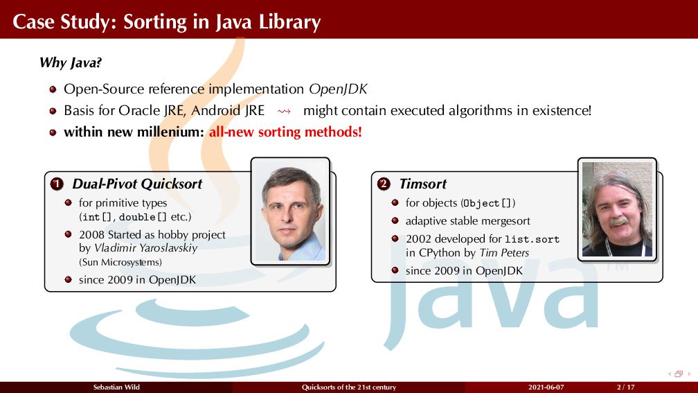
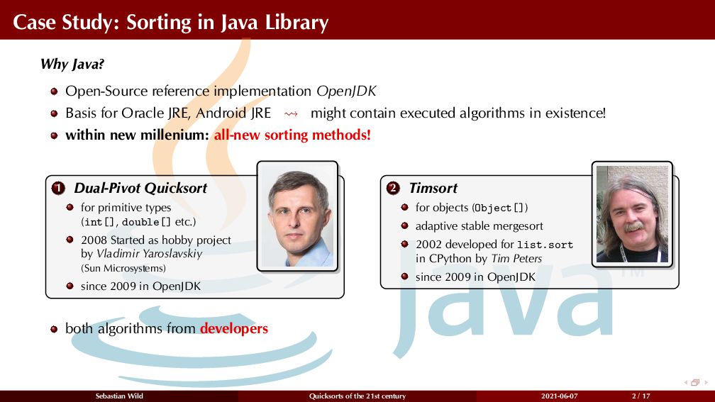
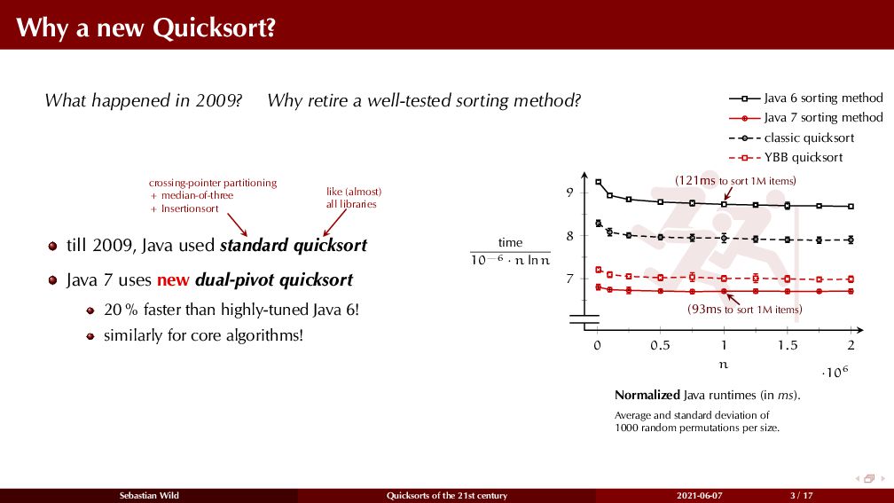
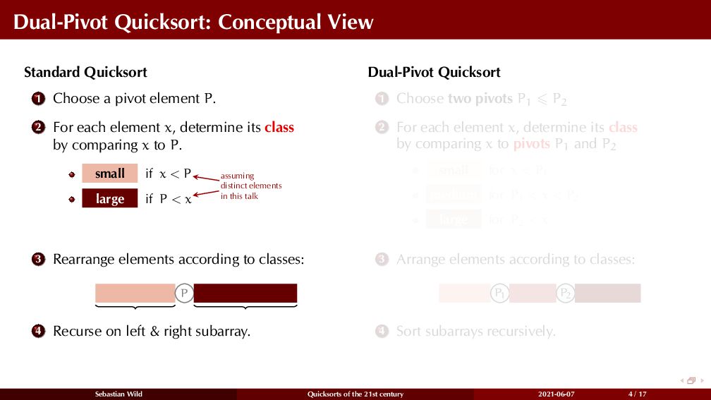
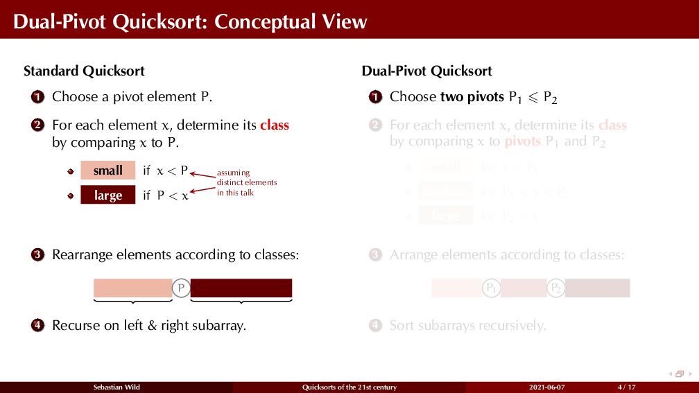
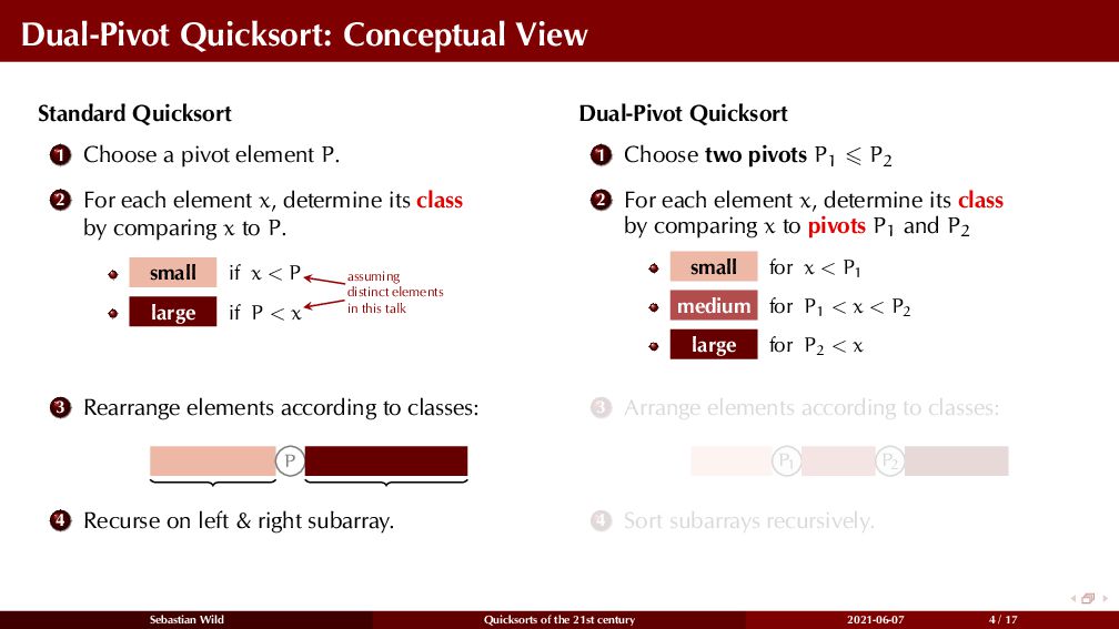
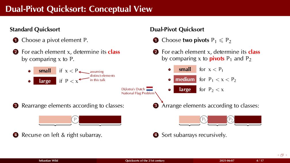
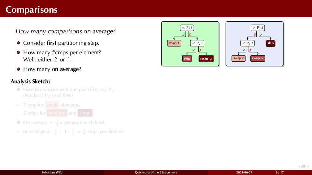
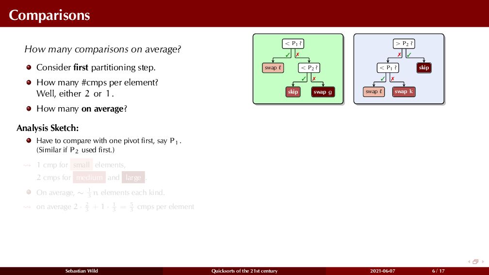
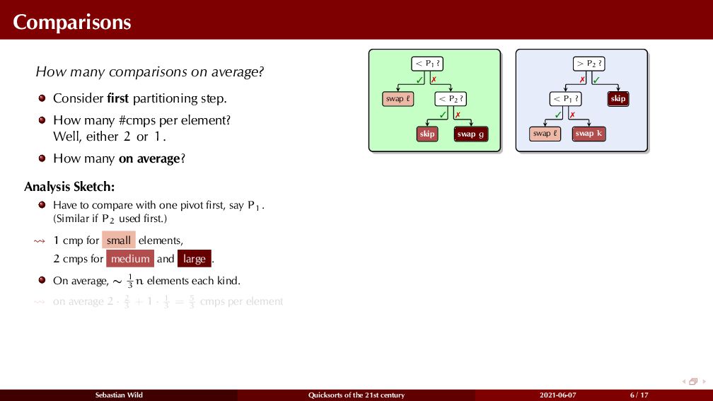
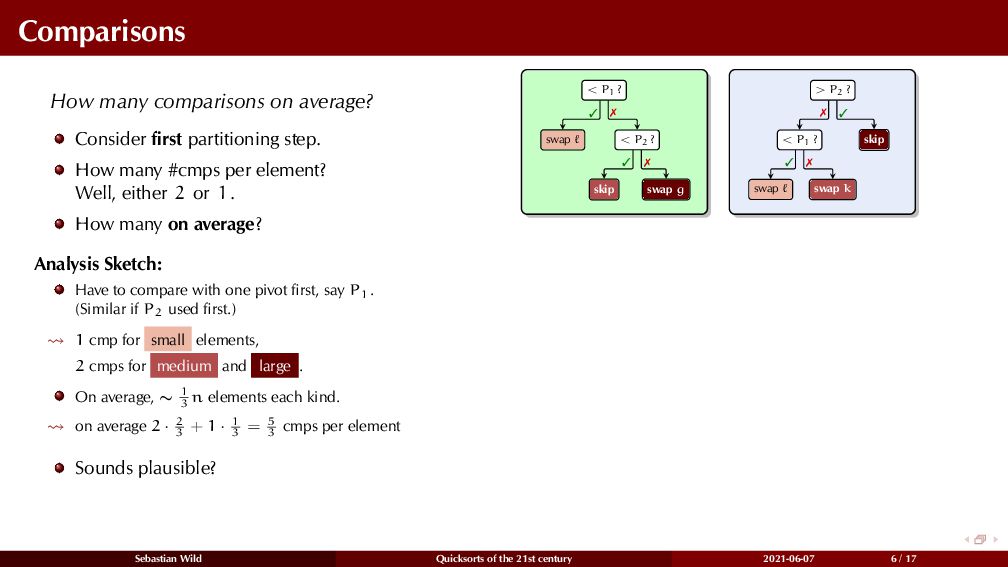
Quicksort is one of most well-understood algorithms – both in terms of theoretical performance guarantees and practical running time – and an implementation of quicksort is part of almost every programming library. While the first 3 decades after quicksort's publication have seen extensive engineering efforts, implementations seemed to have converged to a stable state. But now, there is again excitement within the algorithms community, triggered by the success of a new dual-pivot quicksort introduced in the Java 7 runtime library.
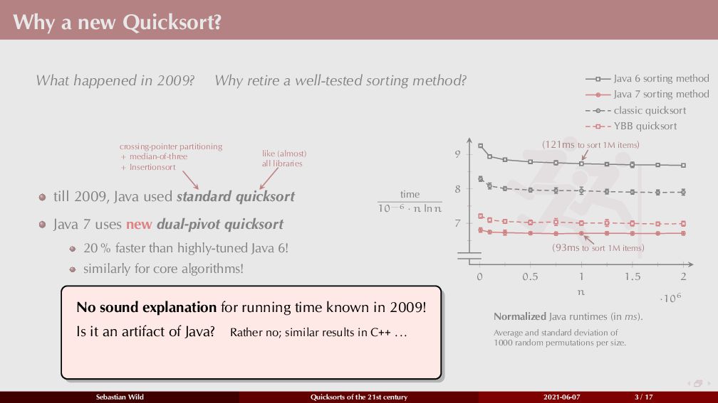
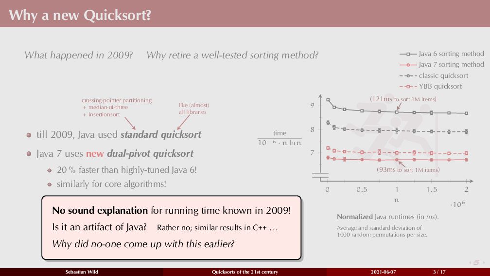
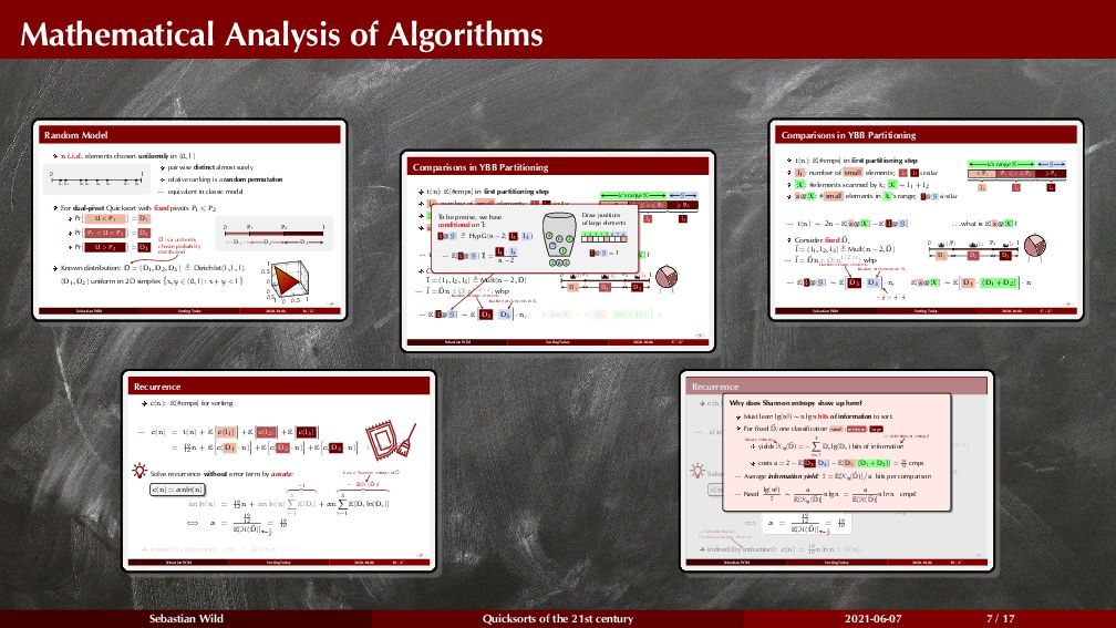
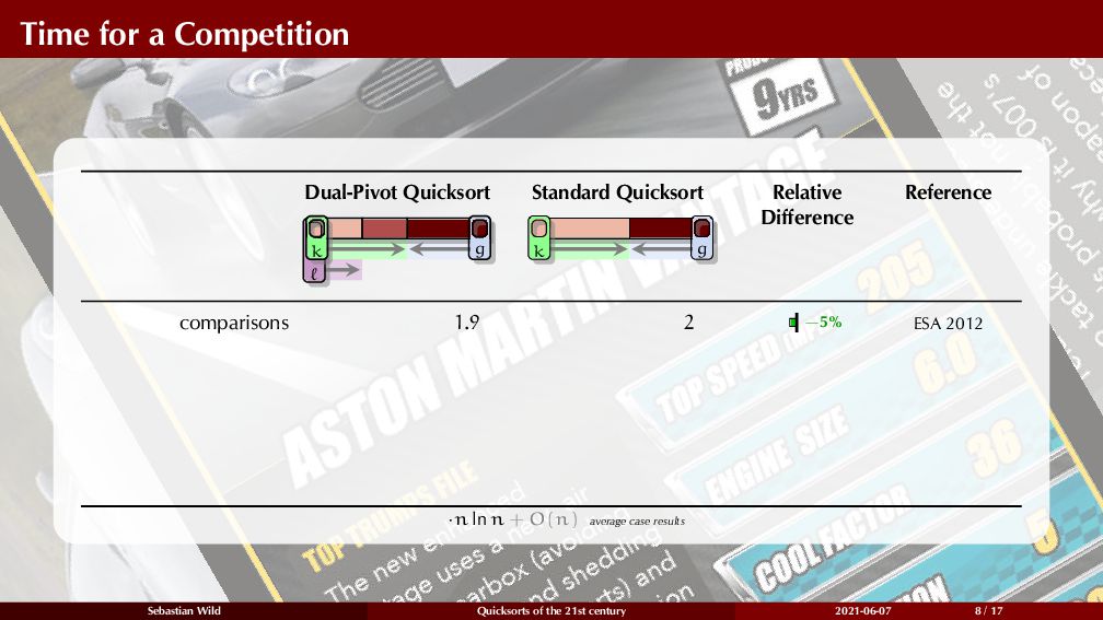
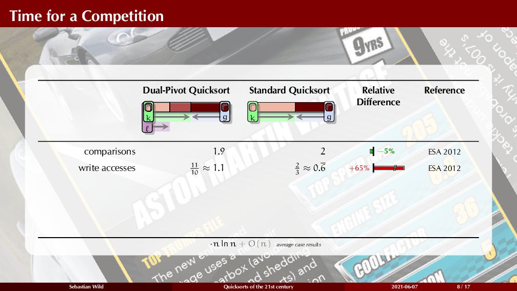
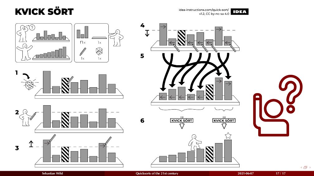
I will introduce this algorithm and present analytical evidence for my hypothesis why (a) dual-pivot quicksort is faster than the previously used (standard) quicksort and (b) why this basic improvement was not already found much earlier. Moreover, I will spotlight new algorithms inspired by quicksort and some unsolved riddles encountered during my decade with quicksort.
This talk was part of the special session celebrating quicksort's 60th birthday during the “Verified software: tools and experiments” workshop at the Isaac Newton Institute (https://www.newton.ac.uk/event/vsow04/).
A video recording of the talk is available here: https://www.newton.ac.uk/seminar/20210607173018001/
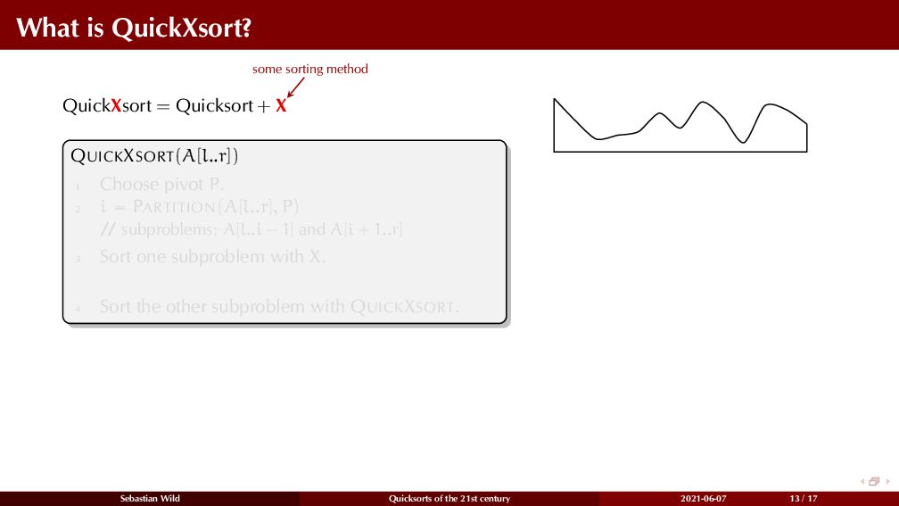
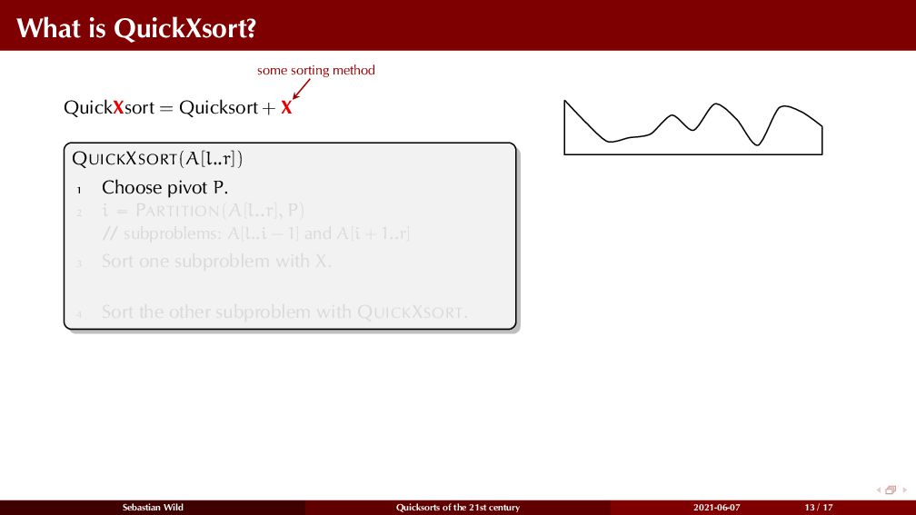
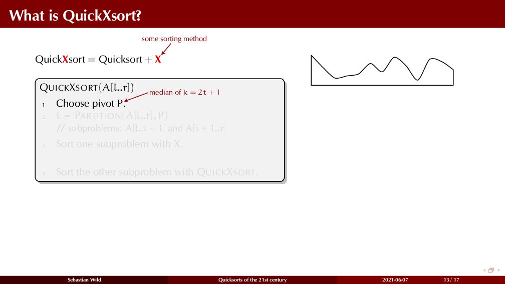
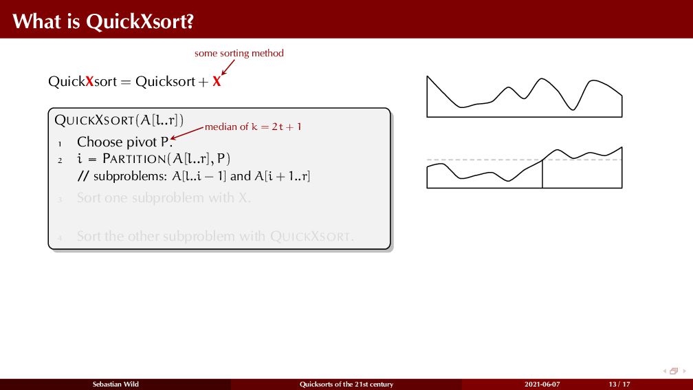
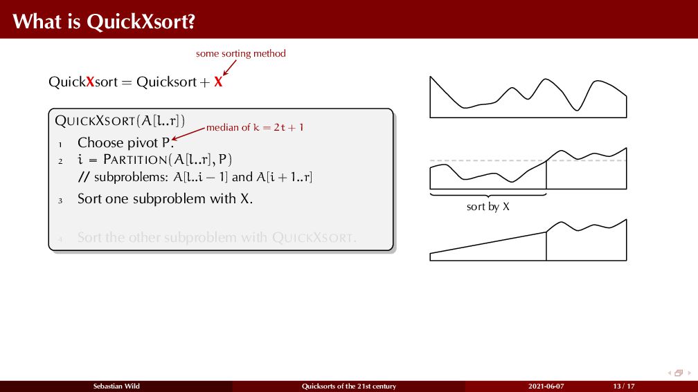
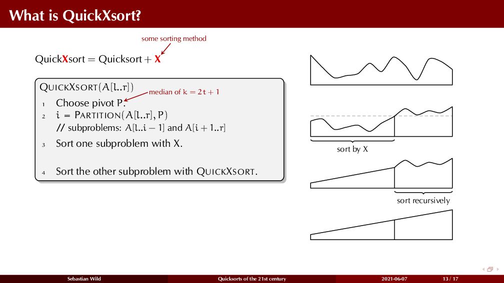
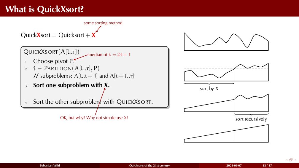
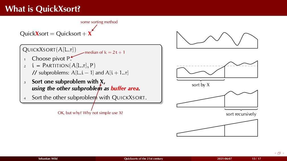
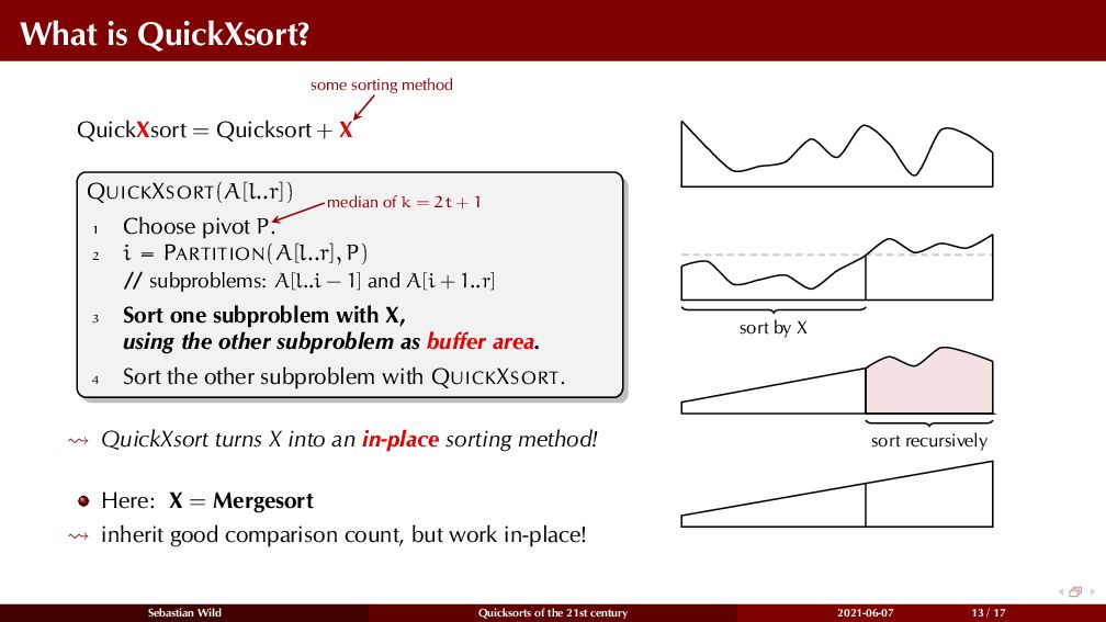
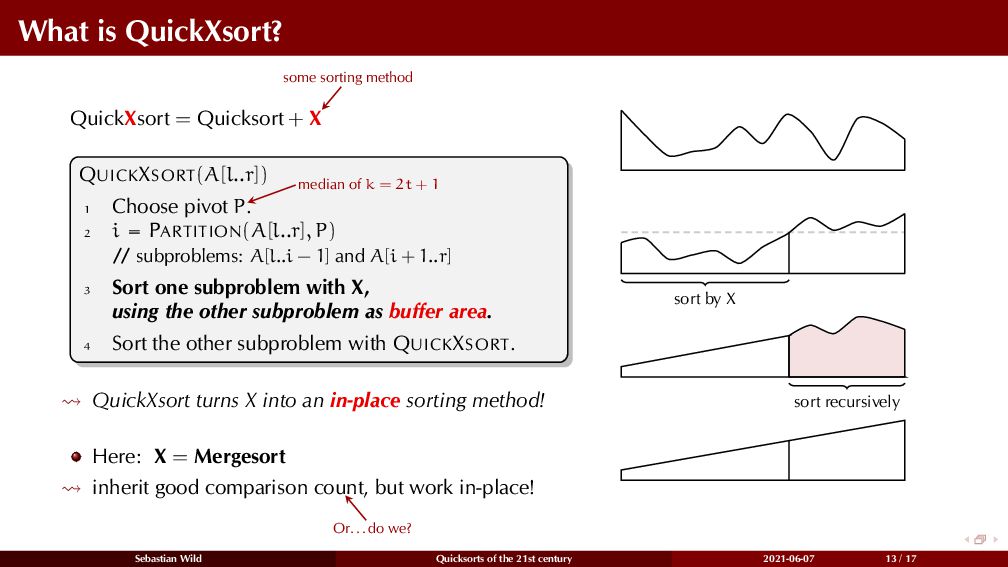
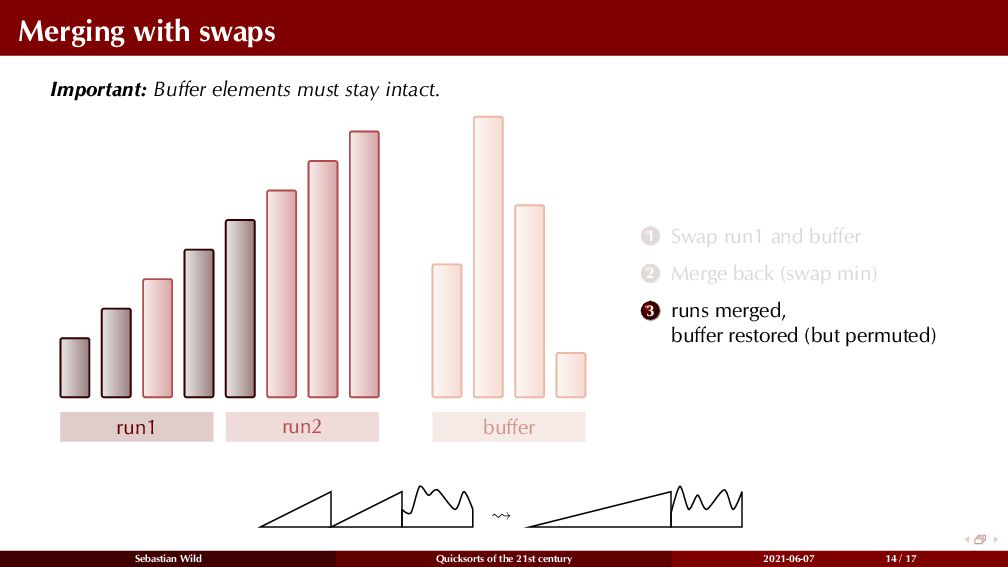
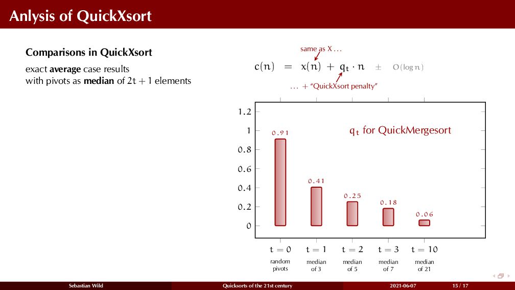
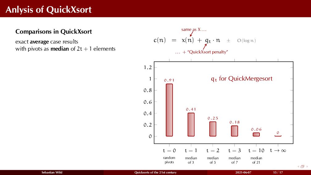
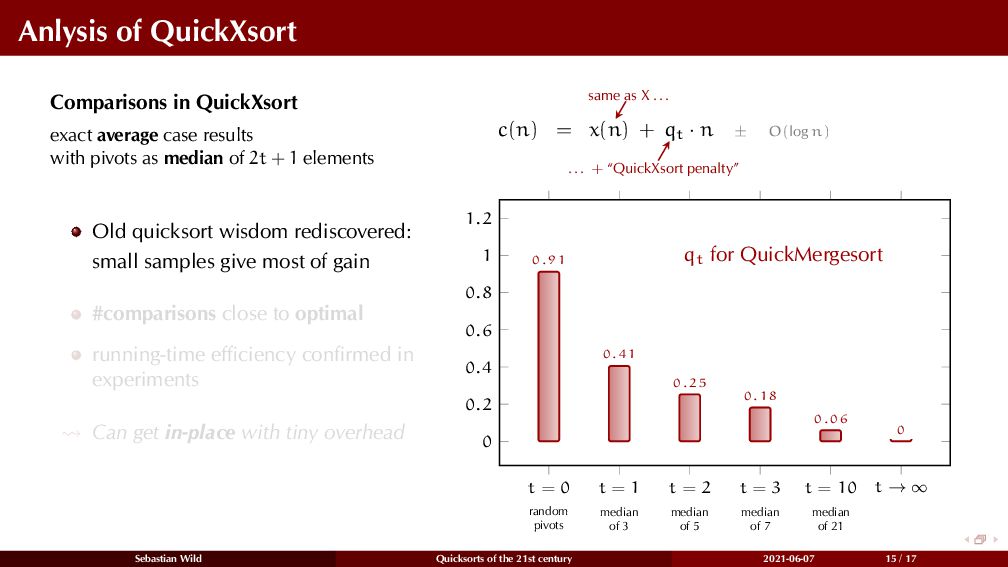
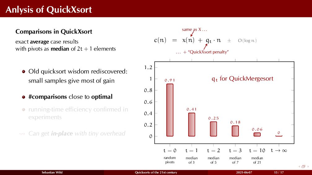
![QuickMergesort QUICKMERGESORT(A[l..r]) 1 Choose pivot P. 2 i = PARTITION(A[l..r],](https://files.speakerdeck.com/presentations/c4080e6c635a44beb180673741d1d407/slide_214.jpg)
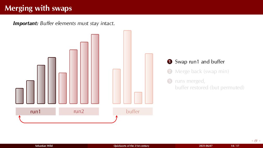
![QuickMergesort QUICKMERGESORT(A[l..r]) 1 Choose pivot P. 2 i = PARTITION(A[l..r],](https://files.speakerdeck.com/presentations/c4080e6c635a44beb180673741d1d407/slide_215.jpg)
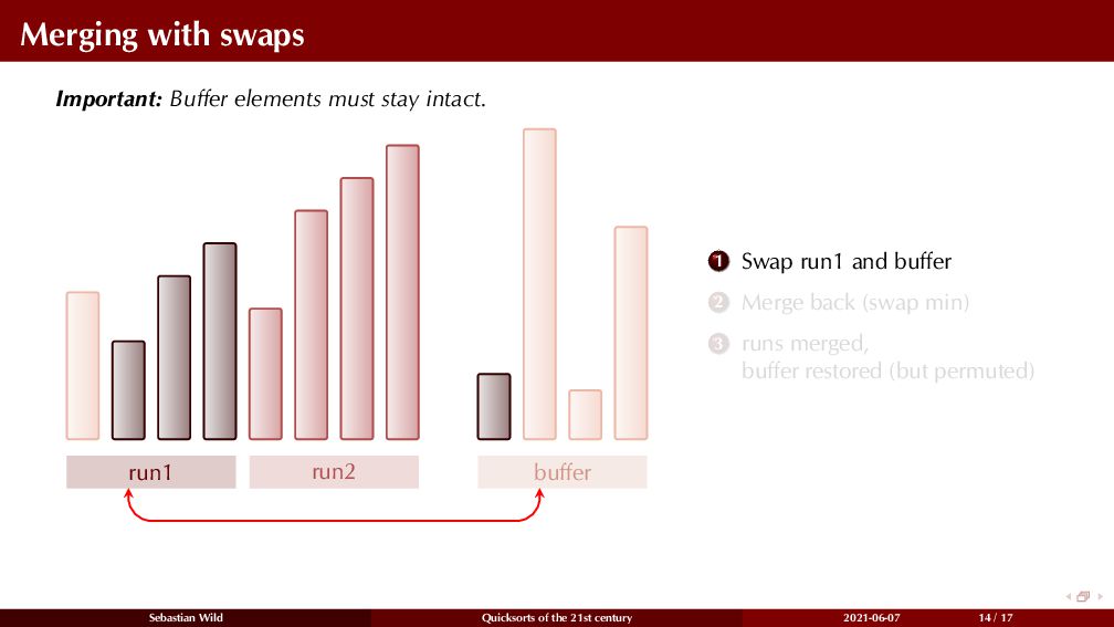
![QuickMergesort QUICKMERGESORT(A[l..r]) 1 Choose pivot P. 2 i = PARTITION(A[l..r],](https://files.speakerdeck.com/presentations/c4080e6c635a44beb180673741d1d407/slide_216.jpg)
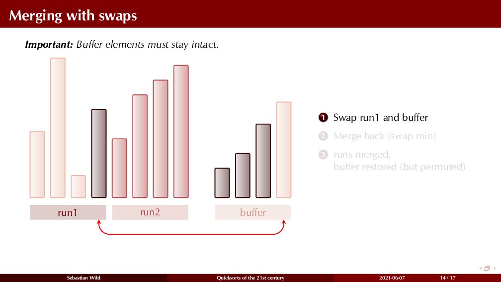
![QuickMergesort QUICKMERGESORT(A[l..r]) 1 Choose pivot P. 2 i = PARTITION(A[l..r],](https://files.speakerdeck.com/presentations/c4080e6c635a44beb180673741d1d407/slide_217.jpg)
![QuickMergesort QUICKMERGESORT(A[l..r]) 1 Choose pivot P. 2 i = PARTITION(A[l..r],](https://files.speakerdeck.com/presentations/c4080e6c635a44beb180673741d1d407/slide_218.jpg)