New solutions at the intersection of black-hole binary simulations and nanohertz gravitational-wave searches

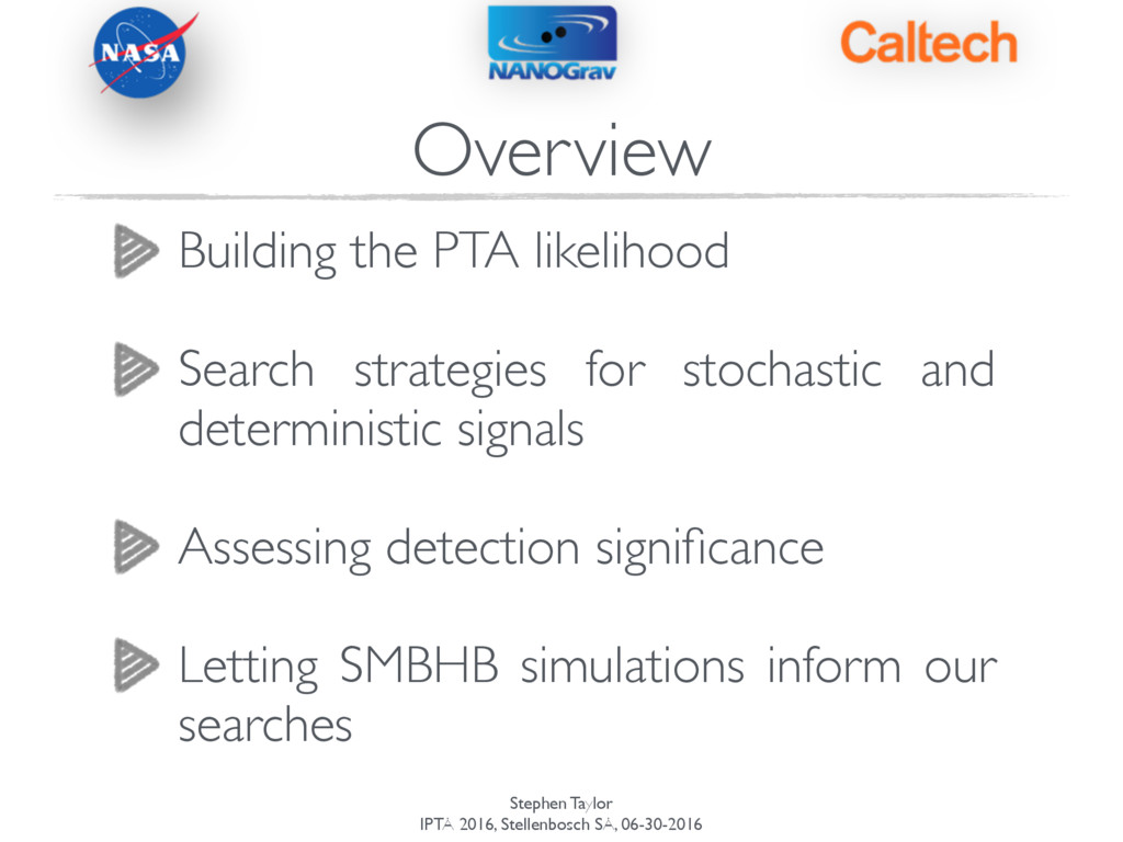
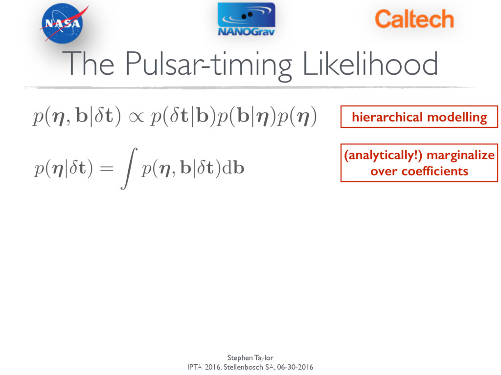
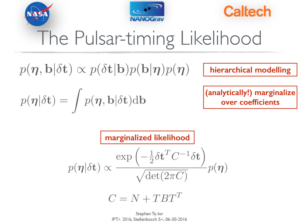
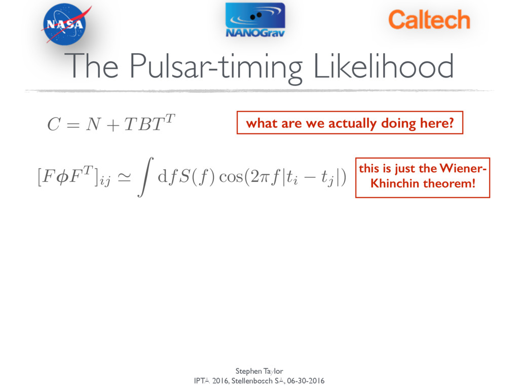
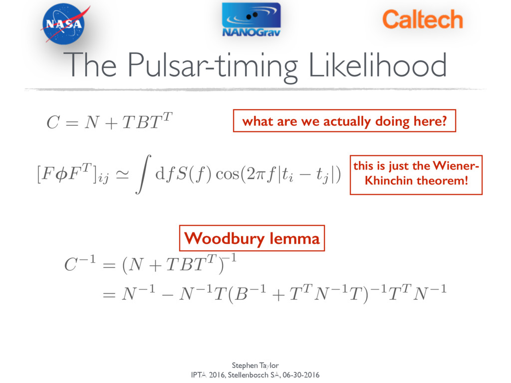
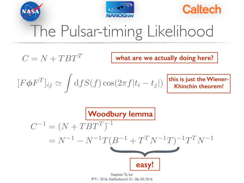
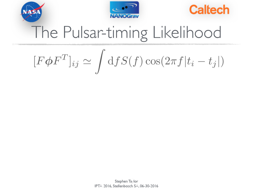
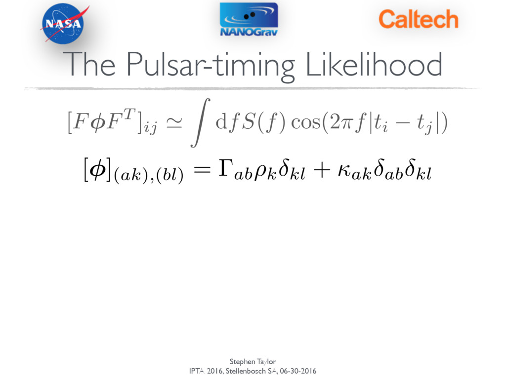
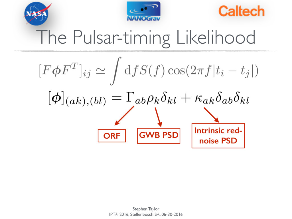
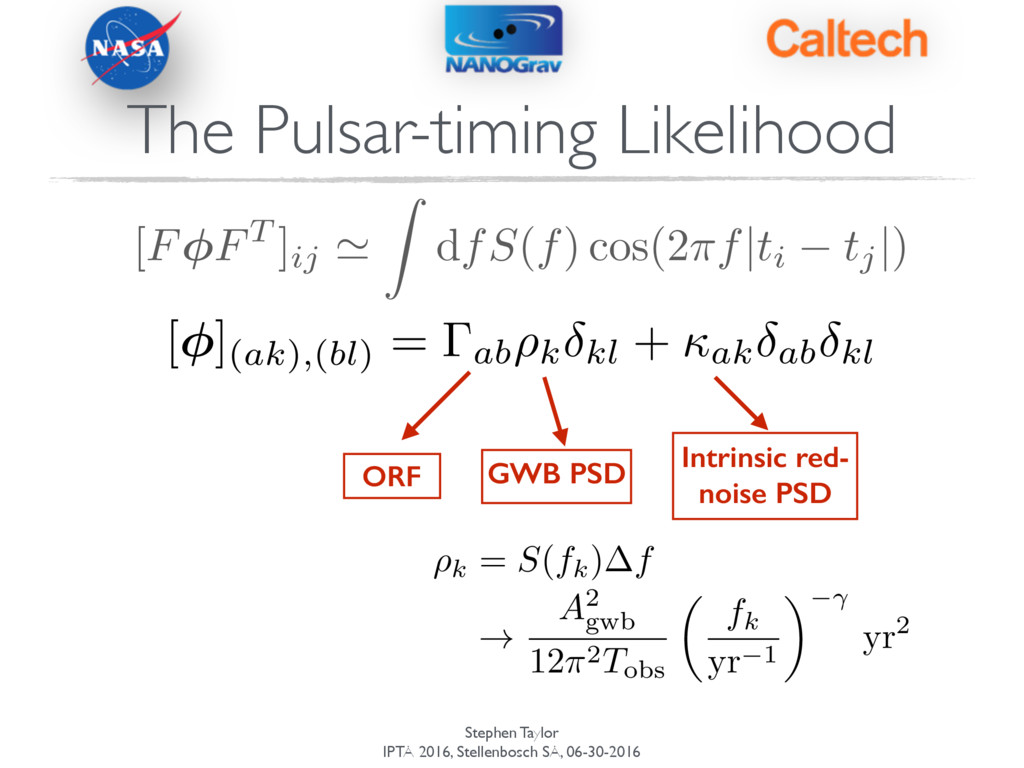
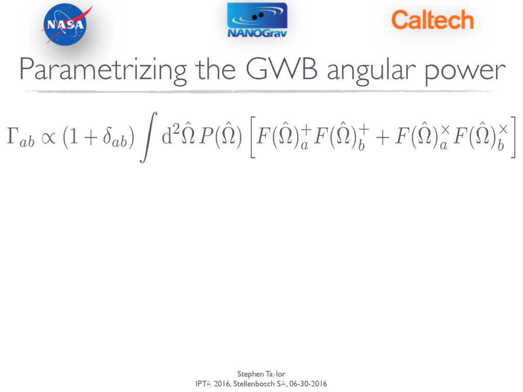
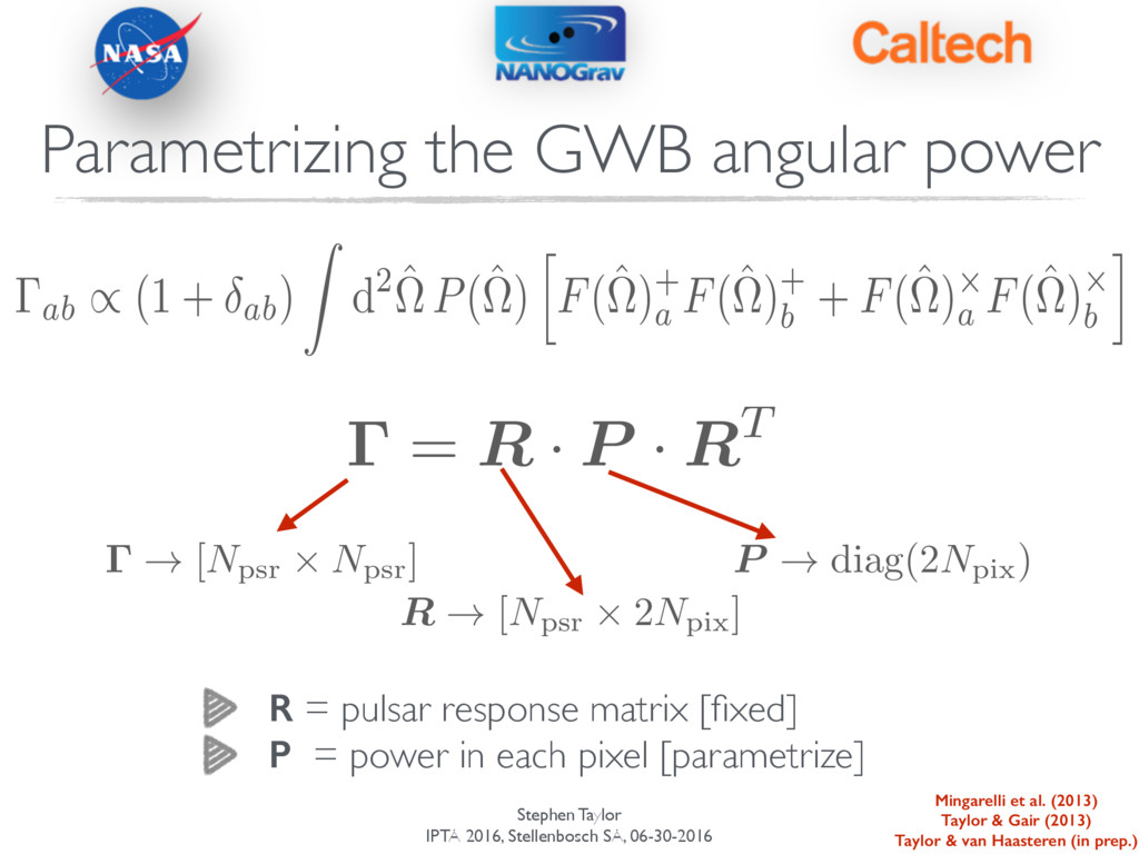
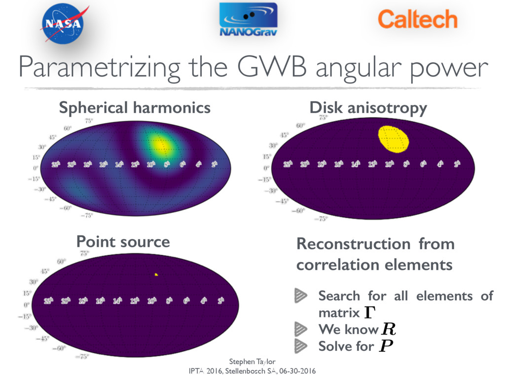
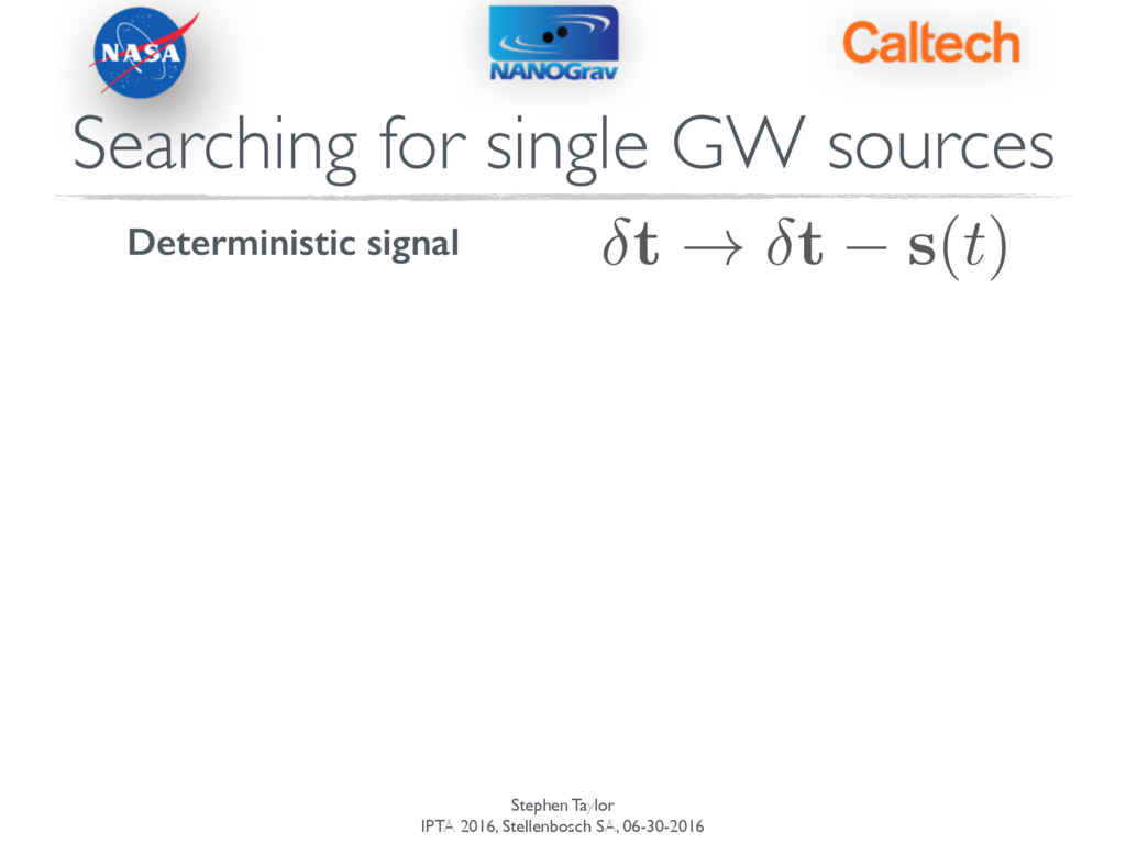
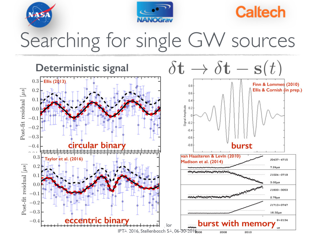
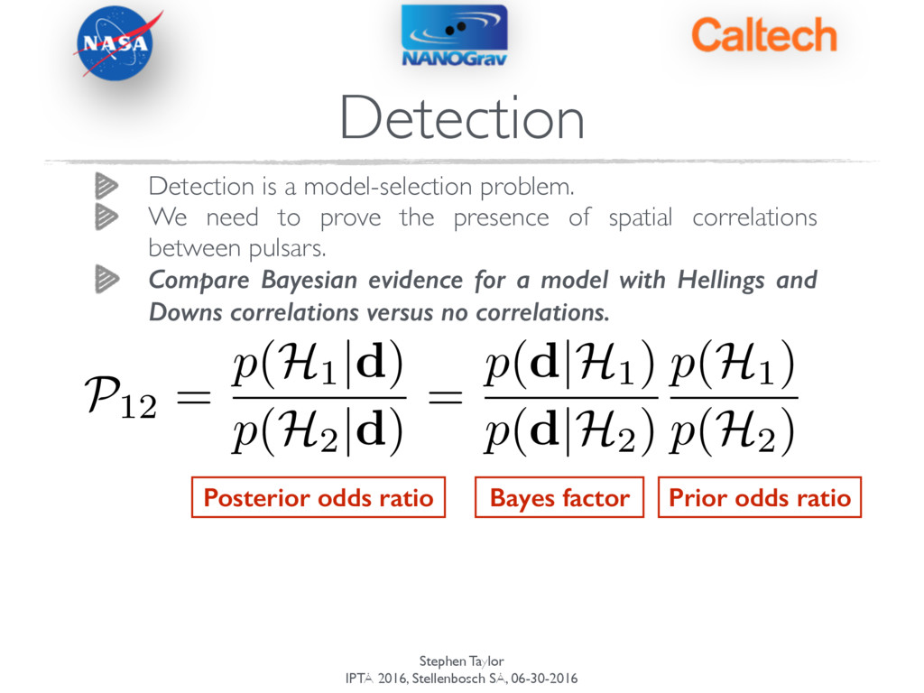
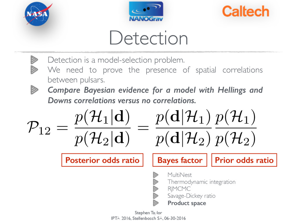
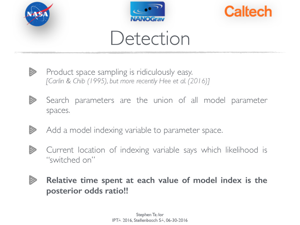
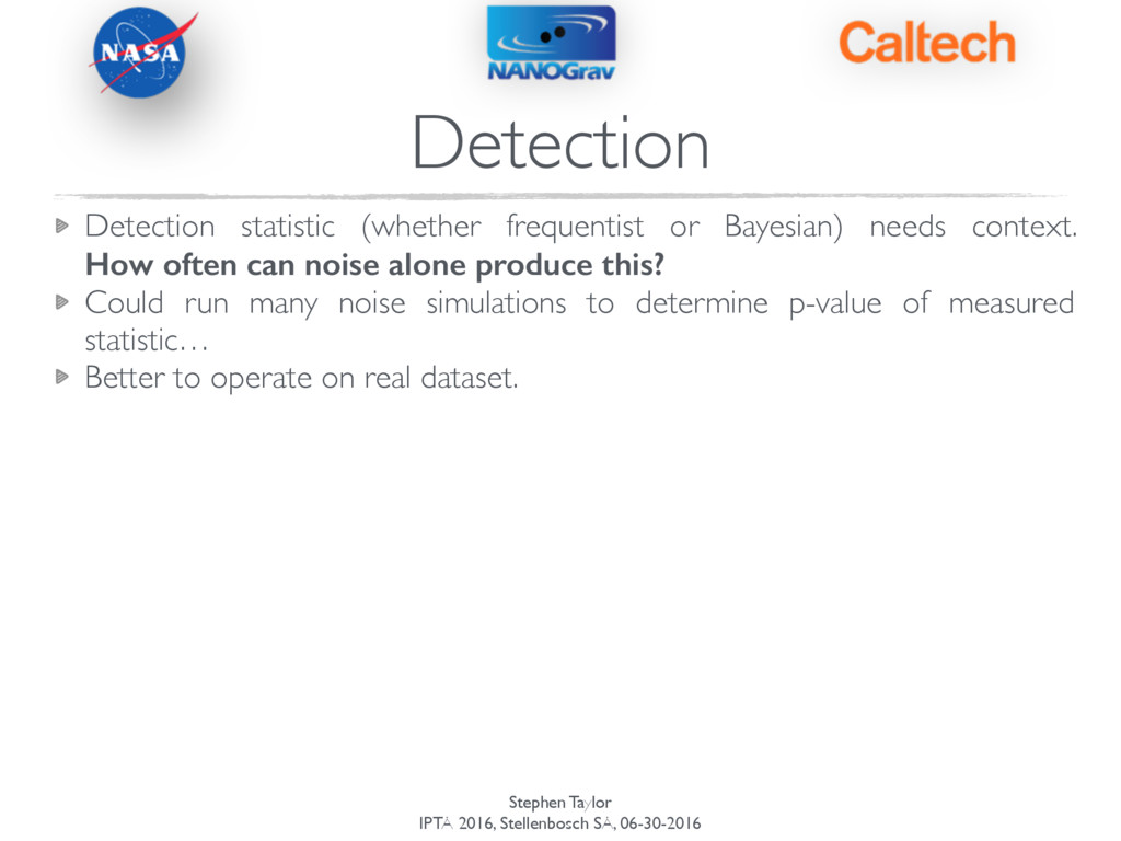
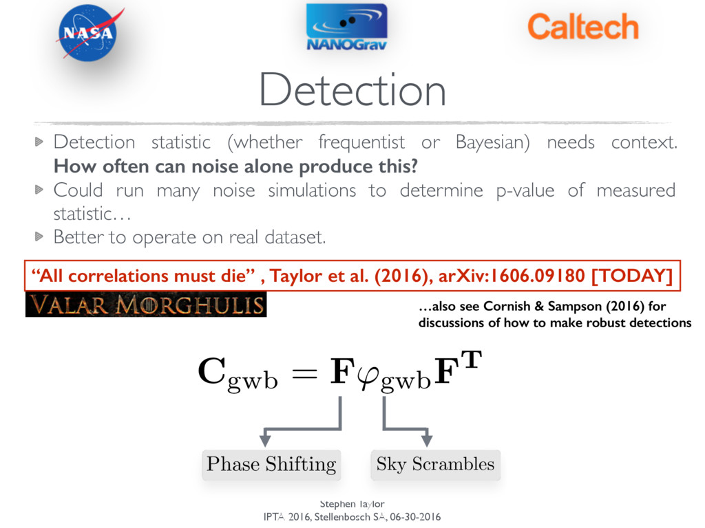
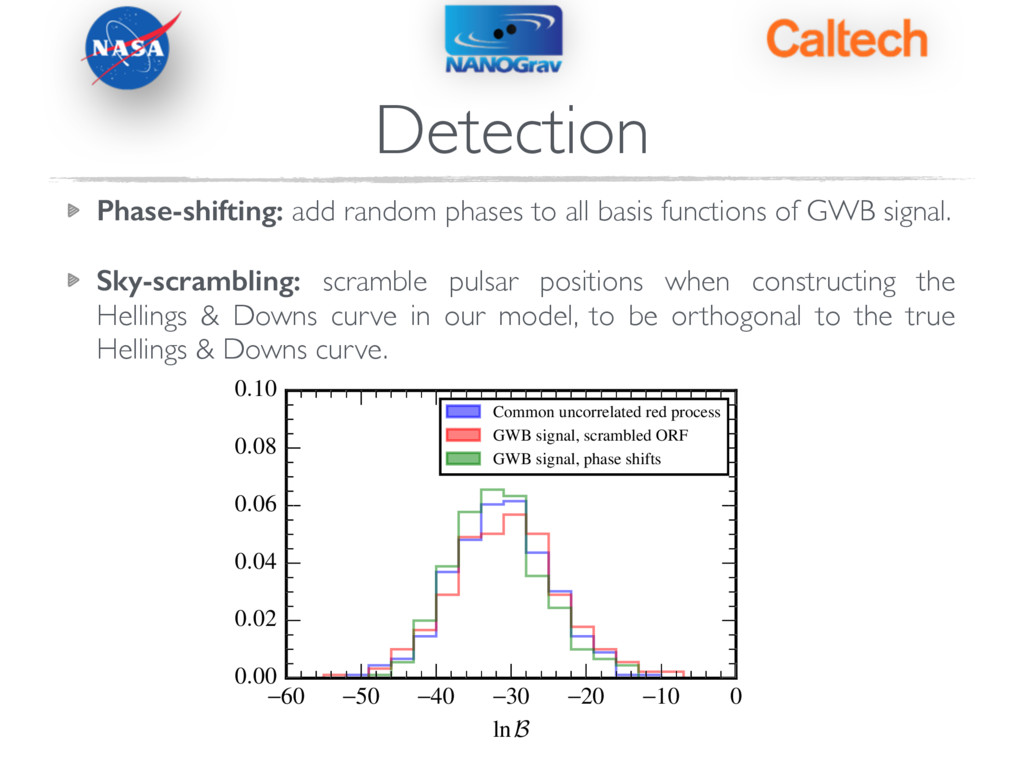
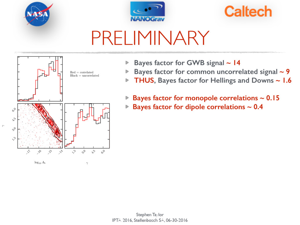
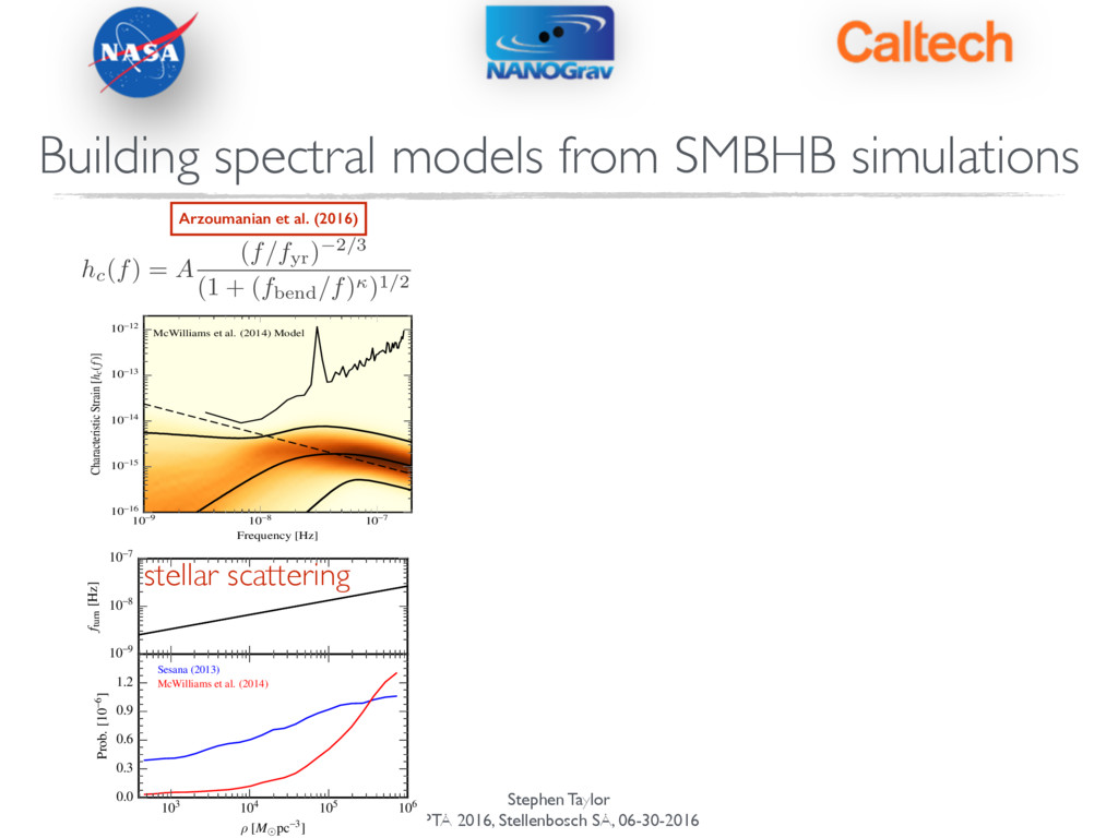
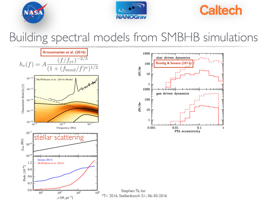
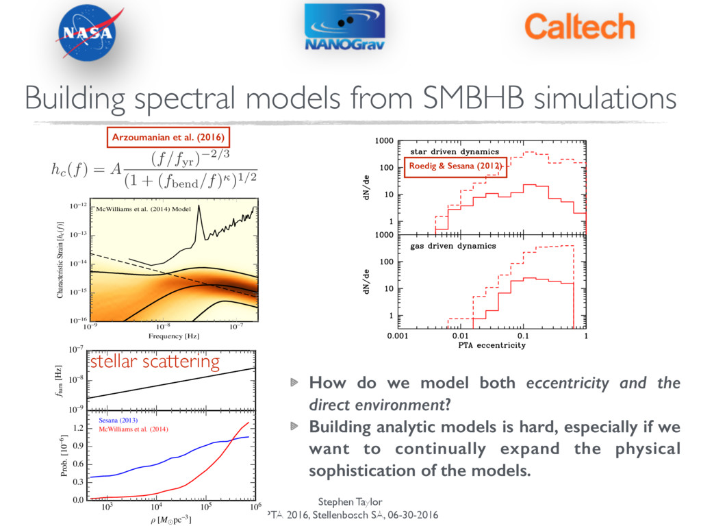
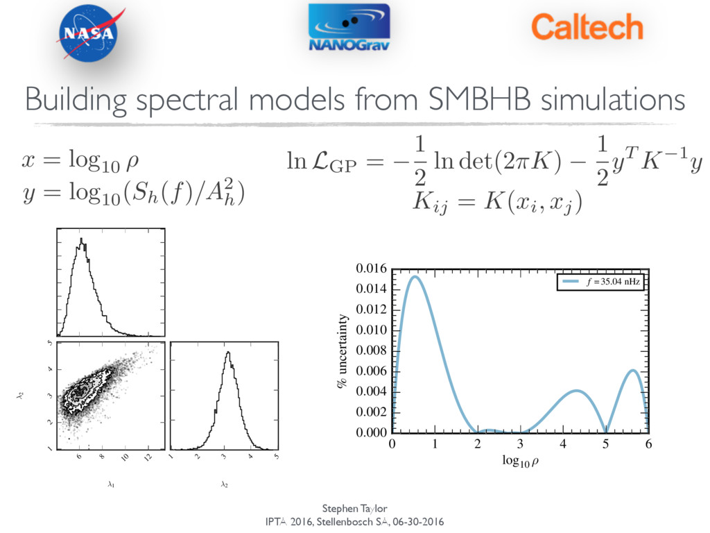
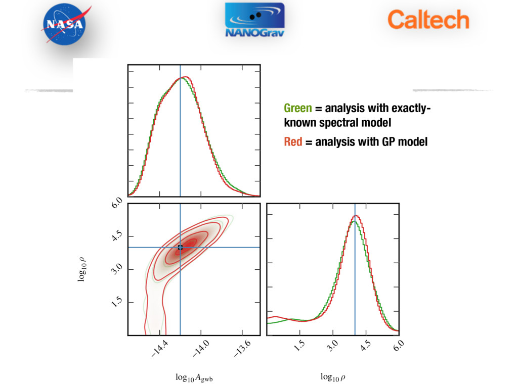
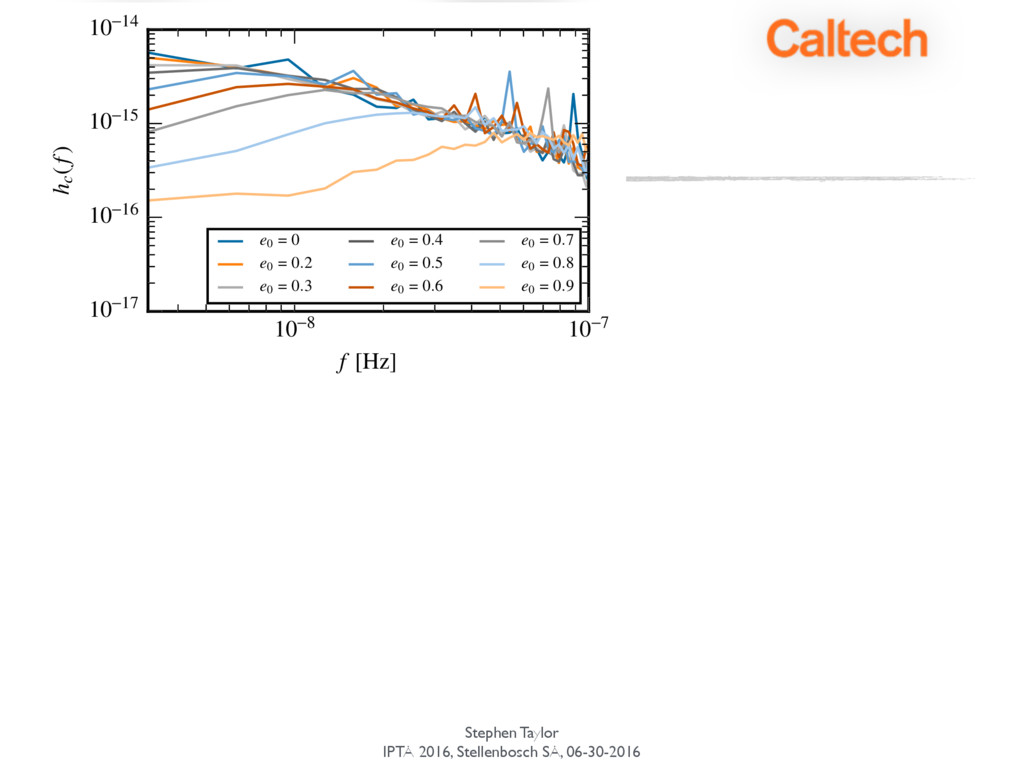
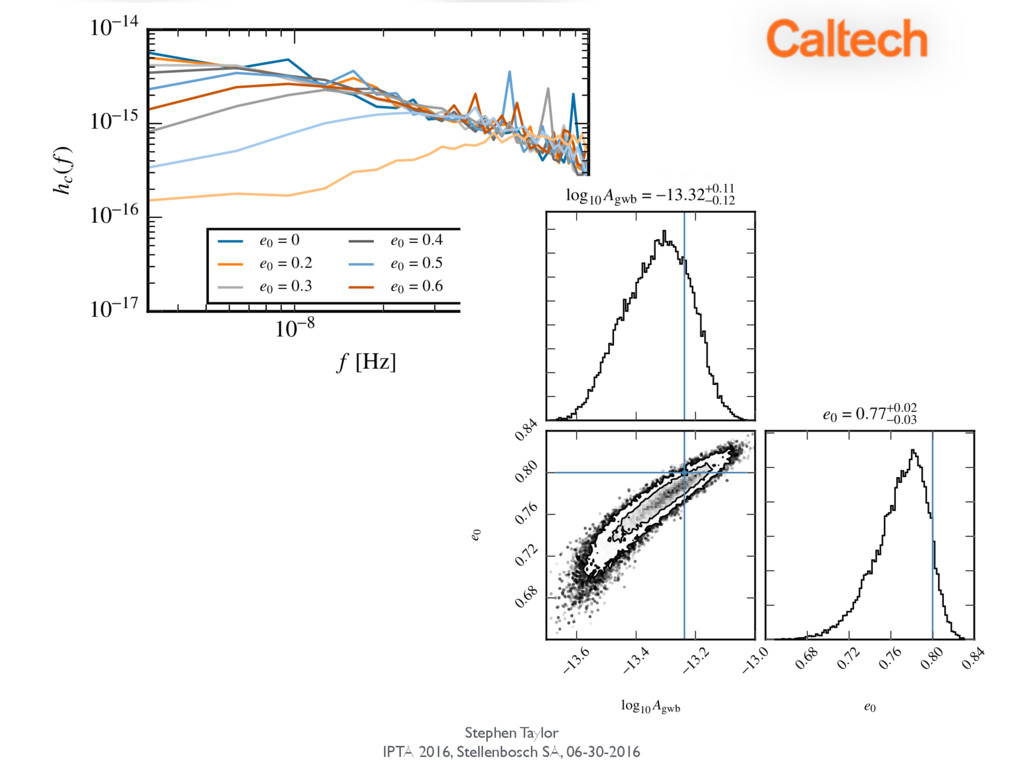
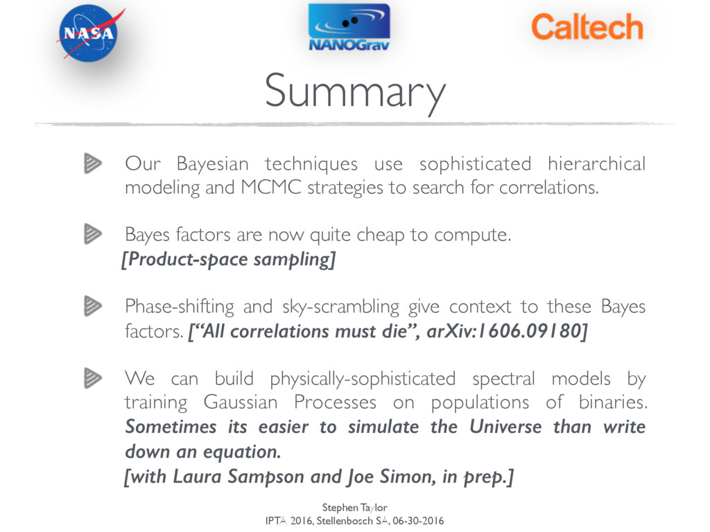
[06/30/2016] An invited talk at the 2016 International Pulsar Timing Array meeting in Stellenbosch, South Africa. I start with an introduction to current data-analysis approaches to pulsar-timing gravitational-wave searches, then discuss how we assess detection significance, and how we can build models based on simulations.

Transcript

1. Stephen Taylor IPTA 2016, Stellenbosch SA, 06-30-2016 © 2016 California Institute of Technology. Government sponsorship acknowledged Stephen R. Taylor New solutions at the intersection of black-hole binary simulations and nanohertz gravitational-wave searches NASA POSTDOCTORAL FELLOW, JET PROPULSION LABORATORY, CALIFORNIA INSTITUTE OF TECHNOLOGY
2. Stephen Taylor IPTA 2016, Stellenbosch SA, 06-30-2016 Building the PTA likelihood ! Search strategies for stochastic and deterministic signals ! Assessing detection significance ! Letting SMBHB simulations inform our searches Overview
3. Stephen Taylor IPTA 2016, Stellenbosch SA, 06-30-2016 The Pulsar-timing Likelihood T = ⇥ M F U ⇤ b = 2 4 ✏ a j 3 5 Tb = M✏ + Fa + Uj p ( t|b ) = exp 1 2 ( t Tb ) TN 1 ( t Tb ) p det(2 ⇡N )
4. Stephen Taylor IPTA 2016, Stellenbosch SA, 06-30-2016 The Pulsar-timing Likelihood T = ⇥ M F U ⇤ b = 2 4 ✏ a j 3 5 Tb = M✏ + Fa + Uj p ( b|⌘ ) = exp 1 2 bT B 1b p det(2 ⇡B ) B = 2 4 1 0 0 0 0 0 0 J 3 5 p ( t|b ) = exp 1 2 ( t Tb ) TN 1 ( t Tb ) p det(2 ⇡N ) everything is a random Gaussian process!
5. Stephen Taylor IPTA 2016, Stellenbosch SA, 06-30-2016 The Pulsar-timing Likelihood p(⌘| t) = Z p(⌘, b| t)db p(⌘, b| t) / p( t|b)p(b|⌘)p(⌘) hierarchical modelling (analytically!) marginalize over coefficients
6. Stephen Taylor IPTA 2016, Stellenbosch SA, 06-30-2016 The Pulsar-timing Likelihood p(⌘| t) = Z p(⌘, b| t)db p(⌘, b| t) / p( t|b)p(b|⌘)p(⌘) p ( ⌘| t ) / exp ⇣ 1 2 tT C 1 t ⌘ p det(2 ⇡C ) p ( ⌘ ) C = N + TBTT hierarchical modelling (analytically!) marginalize over coefficients marginalized likelihood
7. Stephen Taylor IPTA 2016, Stellenbosch SA, 06-30-2016 The Pulsar-timing Likelihood C = N + TBTT what are we actually doing here? this is just the Wiener- Khinchin theorem! [ F FT ]ij ' Z d fS ( f ) cos(2 ⇡f|ti tj | )
8. Stephen Taylor IPTA 2016, Stellenbosch SA, 06-30-2016 The Pulsar-timing Likelihood C = N + TBTT what are we actually doing here? this is just the Wiener- Khinchin theorem! [ F FT ]ij ' Z d fS ( f ) cos(2 ⇡f|ti tj | ) C 1 = (N + TBTT ) = N 1 N 1T(B 1 + TT N 1T) 1TT N 1 Woodbury lemma 1
9. Stephen Taylor IPTA 2016, Stellenbosch SA, 06-30-2016 The Pulsar-timing Likelihood C = N + TBTT what are we actually doing here? this is just the Wiener- Khinchin theorem! [ F FT ]ij ' Z d fS ( f ) cos(2 ⇡f|ti tj | ) C 1 = (N + TBTT ) = N 1 N 1T(B 1 + TT N 1T) 1TT N 1 easy! Woodbury lemma 1
10. Stephen Taylor IPTA 2016, Stellenbosch SA, 06-30-2016 The Pulsar-timing Likelihood Without cross-pulsar correlations [~ms] ! With cross-pulsar correlations [~0.1s]
11. Stephen Taylor IPTA 2016, Stellenbosch SA, 06-30-2016 The Pulsar-timing Likelihood Without cross-pulsar correlations [~ms] ! With cross-pulsar correlations [~0.1s]
12. Stephen Taylor IPTA 2016, Stellenbosch SA, 06-30-2016 The Pulsar-timing Likelihood [ F FT ]ij ' Z d fS ( f ) cos(2 ⇡f|ti tj | )
13. Stephen Taylor IPTA 2016, Stellenbosch SA, 06-30-2016 The Pulsar-timing Likelihood [ F FT ]ij ' Z d fS ( f ) cos(2 ⇡f|ti tj | ) [ ](ak),(bl) = ab⇢k kl + ak ab kl
14. Stephen Taylor IPTA 2016, Stellenbosch SA, 06-30-2016 The Pulsar-timing Likelihood ORF GWB PSD Intrinsic red- noise PSD [ F FT ]ij ' Z d fS ( f ) cos(2 ⇡f|ti tj | ) [ ](ak),(bl) = ab⇢k kl + ak ab kl
15. Stephen Taylor IPTA 2016, Stellenbosch SA, 06-30-2016 The Pulsar-timing Likelihood ORF GWB PSD Intrinsic red- noise PSD [ F FT ]ij ' Z d fS ( f ) cos(2 ⇡f|ti tj | ) [ ](ak),(bl) = ab⇢k kl + ak ab kl ⇢k = S(fk) f ! A2 gwb 12⇡2 T obs ✓ fk yr 1 ◆ yr2
16. Stephen Taylor IPTA 2016, Stellenbosch SA, 06-30-2016 Parametrizing the GWB angular power ab / (1 + ab) Z d2 ˆ ⌦P(ˆ ⌦) h F(ˆ ⌦)+ a F(ˆ ⌦)+ b + F(ˆ ⌦)⇥ a F(ˆ ⌦)⇥ b i
17. Stephen Taylor IPTA 2016, Stellenbosch SA, 06-30-2016 Parametrizing the GWB angular power ab / (1 + ab) Z d2 ˆ ⌦P(ˆ ⌦) h F(ˆ ⌦)+ a F(ˆ ⌦)+ b + F(ˆ ⌦)⇥ a F(ˆ ⌦)⇥ b i = R · P · RT R ! [N psr ⇥ 2N pix ] P ! diag(2N pix ) ! [Npsr ⇥ Npsr] R = pulsar response matrix [fixed] P = power in each pixel [parametrize] Mingarelli et al. (2013) Taylor & Gair (2013) Taylor & van Haasteren (in prep.)
18. Stephen Taylor IPTA 2016, Stellenbosch SA, 06-30-2016 Parametrizing the GWB angular power Spherical harmonics Disk anisotropy Point source Reconstruction from correlation elements Search for all elements of matrix We know Solve for R P
19. Stephen Taylor IPTA 2016, Stellenbosch SA, 06-30-2016 Searching for single GW sources
20. Stephen Taylor IPTA 2016, Stellenbosch SA, 06-30-2016 Searching for single GW sources t ! t s(t) Deterministic signal
21. Stephen Taylor IPTA 2016, Stellenbosch SA, 06-30-2016 Searching for single GW sources t ! t s(t) Deterministic signal 0.4 0.3 0.2 0.1 0.0 0.1 0.2 0.3 Post-fit residual [µs] 0.04 s] 0.4 0.3 0.2 0.1 0.0 0.1 0.2 0.3 Post-fit residual [µs] 53000 53500 54000 54500 55000 55500 56000 56500 0.03 0.02 0.01 0.00 0.01 0.02 0.03 0.04 = srec.(t) strue(t) [µs] 1662 J. B. Wang et al. circular binary eccentric binary burst with memory burst Ellis (2013) Taylor et al. (2016) van Haasteren & Levin (2010) Madison et al. (2014) Finn & Lommen (2010) Ellis & Cornish (in prep.)
22. Stephen Taylor IPTA 2016, Stellenbosch SA, 06-30-2016 Detection Detection is a model-selection problem. We need to prove the presence of spatial correlations between pulsars. Compare Bayesian evidence for a model with Hellings and Downs correlations versus no correlations.
23. Stephen Taylor IPTA 2016, Stellenbosch SA, 06-30-2016 Detection Detection is a model-selection problem. We need to prove the presence of spatial correlations between pulsars. Compare Bayesian evidence for a model with Hellings and Downs correlations versus no correlations. P12 = p(H1 |d) p(H2 |d) = p(d|H1) p(d|H2) p(H1) p(H2) Posterior odds ratio Bayes factor Prior odds ratio
24. Stephen Taylor IPTA 2016, Stellenbosch SA, 06-30-2016 Detection Detection is a model-selection problem. We need to prove the presence of spatial correlations between pulsars. Compare Bayesian evidence for a model with Hellings and Downs correlations versus no correlations. P12 = p(H1 |d) p(H2 |d) = p(d|H1) p(d|H2) p(H1) p(H2) Posterior odds ratio Bayes factor Prior odds ratio MultiNest Thermodynamic integration RJMCMC Savage-Dickey ratio Product space
25. Stephen Taylor IPTA 2016, Stellenbosch SA, 06-30-2016 Detection Product space sampling is ridiculously easy. [Carlin & Chib (1995), but more recently Hee et al. (2016)] ! Search parameters are the union of all model parameter spaces. ! Add a model indexing variable to parameter space. ! Current location of indexing variable says which likelihood is “switched on” ! Relative time spent at each value of model index is the posterior odds ratio!!
26. Stephen Taylor IPTA 2016, Stellenbosch SA, 06-30-2016 Detection Detection statistic (whether frequentist or Bayesian) needs context. How often can noise alone produce this? Could run many noise simulations to determine p-value of measured statistic… Better to operate on real dataset.
27. Stephen Taylor IPTA 2016, Stellenbosch SA, 06-30-2016 Cgwb = F'gwbFT Phase Shifting Sky Scrambles …also see Cornish & Sampson (2016) for discussions of how to make robust detections Detection Detection statistic (whether frequentist or Bayesian) needs context. How often can noise alone produce this? Could run many noise simulations to determine p-value of measured statistic… Better to operate on real dataset. “All correlations must die” , Taylor et al. (2016), arXiv:1606.09180 [TODAY]
28. Stephen Taylor IPTA 2016, Stellenbosch SA, 06-30-2016 Detection -60 -50 -40 -30 -20 -10 0 lnB 0.00 0.02 0.04 0.06 0.08 0.10 Common uncorrelated red process GWB signal, scrambled ORF GWB signal, phase shifts Phase-shifting: add random phases to all basis functions of GWB signal. ! Sky-scrambling: scramble pulsar positions when constructing the Hellings & Downs curve in our model, to be orthogonal to the true Hellings & Downs curve.
29. Stephen Taylor IPTA 2016, Stellenbosch SA, 06-30-2016 PRELIMINARY 17 16 15 14 log10 Ah 1.5 3.0 4.5 6.0 1.5 3.0 4.5 6.0 Red = correlated Black = uncorrelated Bayes factor for GWB signal ~ 14 Bayes factor for common uncorrelated signal ~ 9 THUS, Bayes factor for Hellings and Downs ~ 1.6 ! Bayes factor for monopole correlations ~ 0.15 Bayes factor for dipole correlations ~ 0.4
30. Stephen Taylor IPTA 2016, Stellenbosch SA, 06-30-2016 PRELIMINARY -1.5 -1.0 -0.5 0.0 0.5 1.0 1.5 lnB 0.0 0.2 0.4 0.6 0.8 1.0 1.2 1.4 GWB signal, phase shifts 17 16 15 14 log10 Ah 1.5 3.0 4.5 6.0 1.5 3.0 4.5 6.0 Red = correlated Black = uncorrelated Bayes factor for GWB signal ~ 14 Bayes factor for common uncorrelated signal ~ 9 THUS, Bayes factor for Hellings and Downs ~ 1.6 ! Bayes factor for monopole correlations ~ 0.15 Bayes factor for dipole correlations ~ 0.4
31. Stephen Taylor IPTA 2016, Stellenbosch SA, 06-30-2016 Building spectral models from SMBHB simulations 12 10-9 10-8 10-7 Frequency [Hz] 10-16 10-15 10-14 10-13 10-12 Characteristic Strain [hc(f)] McWilliams et al. (2014) Model Figure 5. Probability density plots of the recovered GWB spectra for models A and B using the broken-power-law model parameterized by (Agw, fbend, and ) as discussed in the text. The thick black lines indicate the 95% credible region and median of the GWB spectrum. The dashed line shows the 95% upper limit on the amplitude of purely GW-driven spectrum using the Gaussian priors on the amplitude from models A and B, respectively. The thin black curve shows the 95% upper limit on the GWB spectrum from the spectral analysis. 16 10-9 10-8 10-7 fturn [Hz] 103 104 105 106 ⇢ [M pc-3] 0.0 0.3 0.6 0.9 1.2 Prob. [10-6] Sesana (2013) McWilliams et al. (2014) stellar scattering hc(f) = A (f/fyr) 2/3 (1 + (fbend/f))1/2 Arzoumanian et al. (2016)
32. Stephen Taylor IPTA 2016, Stellenbosch SA, 06-30-2016 Building spectral models from SMBHB simulations 12 10-9 10-8 10-7 Frequency [Hz] 10-16 10-15 10-14 10-13 10-12 Characteristic Strain [hc(f)] McWilliams et al. (2014) Model Figure 5. Probability density plots of the recovered GWB spectra for models A and B using the broken-power-law model parameterized by (Agw, fbend, and ) as discussed in the text. The thick black lines indicate the 95% credible region and median of the GWB spectrum. The dashed line shows the 95% upper limit on the amplitude of purely GW-driven spectrum using the Gaussian priors on the amplitude from models A and B, respectively. The thin black curve shows the 95% upper limit on the GWB spectrum from the spectral analysis. 16 10-9 10-8 10-7 fturn [Hz] 103 104 105 106 ⇢ [M pc-3] 0.0 0.3 0.6 0.9 1.2 Prob. [10-6] Sesana (2013) McWilliams et al. (2014) stellar scattering hc(f) = A (f/fyr) 2/3 (1 + (fbend/f))1/2 Figure 2. Eccentricity population of MBHBs detectable by ELISA/NGO and PTAs, expected in stellar and gaseous environments. Left panel: The solid histograms represent the efficient models whereas the dashed histograms are for the inefficient models. Right panel: solid his- tograms include all sources producing timing residuals above 3 ns, dashed histograms include all sources producing residual above 10 ns. mechanism (gas/star) we consider two scenarios (efficient/inefficient), to give an idea of the expected eccentricity range. The models are the following (i) gas-efficient: α = 0.3, ˙ m = 1. The migration timescale is maximized for this high values of the disc parameters, and the decoupling occurs in the very late stage of the MBHB evolution; Roedig & Sesana (2012) Arzoumanian et al. (2016)
33. Stephen Taylor IPTA 2016, Stellenbosch SA, 06-30-2016 Building spectral models from SMBHB simulations 12 10-9 10-8 10-7 Frequency [Hz] 10-16 10-15 10-14 10-13 10-12 Characteristic Strain [hc(f)] McWilliams et al. (2014) Model Figure 5. Probability density plots of the recovered GWB spectra for models A and B using the broken-power-law model parameterized by (Agw, fbend, and ) as discussed in the text. The thick black lines indicate the 95% credible region and median of the GWB spectrum. The dashed line shows the 95% upper limit on the amplitude of purely GW-driven spectrum using the Gaussian priors on the amplitude from models A and B, respectively. The thin black curve shows the 95% upper limit on the GWB spectrum from the spectral analysis. 16 10-9 10-8 10-7 fturn [Hz] 103 104 105 106 ⇢ [M pc-3] 0.0 0.3 0.6 0.9 1.2 Prob. [10-6] Sesana (2013) McWilliams et al. (2014) stellar scattering hc(f) = A (f/fyr) 2/3 (1 + (fbend/f))1/2 Figure 2. Eccentricity population of MBHBs detectable by ELISA/NGO and PTAs, expected in stellar and gaseous environments. Left panel: The solid histograms represent the efficient models whereas the dashed histograms are for the inefficient models. Right panel: solid his- tograms include all sources producing timing residuals above 3 ns, dashed histograms include all sources producing residual above 10 ns. mechanism (gas/star) we consider two scenarios (efficient/inefficient), to give an idea of the expected eccentricity range. The models are the following (i) gas-efficient: α = 0.3, ˙ m = 1. The migration timescale is maximized for this high values of the disc parameters, and the decoupling occurs in the very late stage of the MBHB evolution; Roedig & Sesana (2012) Arzoumanian et al. (2016) How do we model both eccentricity and the direct environment? Building analytic models is hard, especially if we want to continually expand the physical sophistication of the models.
34. Stephen Taylor IPTA 2016, Stellenbosch SA, 06-30-2016 Building spectral models from SMBHB simulations
35. Stephen Taylor IPTA 2016, Stellenbosch SA, 06-30-2016 Gaussian Process Interpolation •Run a small number of expensive SMBHB population simulations. •Learn the shape of the spectrum at different physical parameter values. •Learn the spectral variance due to finiteness of the SMBHB population. ! •We have a predictor for the shape of the spectrum, AND a measure of the uncertainty from the interpolation scheme. Building spectral models from SMBHB simulations
36. Stephen Taylor IPTA 2016, Stellenbosch SA, 06-30-2016 10-8 10-7 f [Hz] 10-1 100 101 hc(f) ⇢ = 100M pc-3 ⇢ = 500 ⇢ = 1000 ⇢ = 105 ⇢ = 106 /Ah /Ah Building spectral models from SMBHB simulations
37. Stephen Taylor IPTA 2016, Stellenbosch SA, 06-30-2016 10-8 10-7 f [Hz] 10-1 100 101 hc(f) ⇢ = 100M pc-3 ⇢ = 500 ⇢ = 1000 ⇢ = 105 ⇢ = 106 /Ah 10-8 10-7 f [Hz] 10-1 100 101 hc(f) ⇢ = 100M pc-3 ⇢ = 500 ⇢ = 1000 ⇢ = 105 ⇢ = 106 /Ah Building spectral models from SMBHB simulations
38. Stephen Taylor IPTA 2016, Stellenbosch SA, 06-30-2016 • Gaussian Process trained at a few stellar density values. • We can predict the spectral shape at any stellar density value! • Carry the interpolation uncertainty forward into our GW inference. 6 8 10 12 1 1 2 3 4 5 2 1 2 3 4 5 2 x = log10 ⇢ y = log10( Sh( f ) /A2 h) ln LGP = 1 2 ln det(2⇡K) 1 2 yT K 1y Kij = K ( xi, xj) Building spectral models from SMBHB simulations
39. Stephen Taylor IPTA 2016, Stellenbosch SA, 06-30-2016 • Gaussian Process trained at a few stellar density values. • We can predict the spectral shape at any stellar density value! • Carry the interpolation uncertainty forward into our GW inference. 6 8 10 12 1 1 2 3 4 5 2 1 2 3 4 5 2 0 1 2 3 4 5 6 log10 ⇢ 0.000 0.002 0.004 0.006 0.008 0.010 0.012 0.014 0.016 % uncertainty f =35.04 nHz x = log10 ⇢ y = log10( Sh( f ) /A2 h) ln LGP = 1 2 ln det(2⇡K) 1 2 yT K 1y Kij = K ( xi, xj) Building spectral models from SMBHB simulations
40. Stephen Taylor IPTA 2016, Stellenbosch SA, 06-30-2016 -14.4 -14.0 -13.6 log10 Agwb 1.5 3.0 4.5 6.0 log10 ⇢ 1.5 3.0 4.5 6.0 log10 ⇢ Green = analysis with exactly- known spectral model Red = analysis with GP model
41. Stephen Taylor IPTA 2016, Stellenbosch SA, 06-30-2016 10-8 10-7 f [Hz] 10-17 10-16 10-15 10-14 hc(f) e0 = 0 e0 = 0.2 e0 = 0.3 e0 = 0.4 e0 = 0.5 e0 = 0.6 e0 = 0.7 e0 = 0.8 e0 = 0.9
42. Stephen Taylor IPTA 2016, Stellenbosch SA, 06-30-2016 10-8 10-7 f [Hz] 10-17 10-16 10-15 10-14 hc(f) e0 = 0 e0 = 0.2 e0 = 0.3 e0 = 0.4 e0 = 0.5 e0 = 0.6 e0 = 0.7 e0 = 0.8 e0 = 0.9 log10 Agwb = -13.32+0.11 -0.12 -13.6 -13.4 -13.2 -13.0 log10 Agwb 0.68 0.72 0.76 0.80 0.84 e0 0.68 0.72 0.76 0.80 0.84 e0 e0 = 0.77+0.02 -0.03
43. Stephen Taylor IPTA 2016, Stellenbosch SA, 06-30-2016 Summary Our Bayesian techniques use sophisticated hierarchical modeling and MCMC strategies to search for correlations. ! Bayes factors are now quite cheap to compute. [Product-space sampling] ! Phase-shifting and sky-scrambling give context to these Bayes factors. [“All correlations must die”, arXiv:1606.09180] ! We can build physically-sophisticated spectral models by training Gaussian Processes on populations of binaries. Sometimes its easier to simulate the Universe than write down an equation. [with Laura Sampson and Joe Simon, in prep.]