Change in Available Golden Golden-cheeked Warbler Habitat Through Time: An Assessment of Change in Mature Central Texas Juniper Juniper-Oak Woodlands

By Nancy A. Heger and Tom Hayes
NAH: Texas State University and TPWD
TH: Environmental Conservation Alliance, Inc.

Transcript

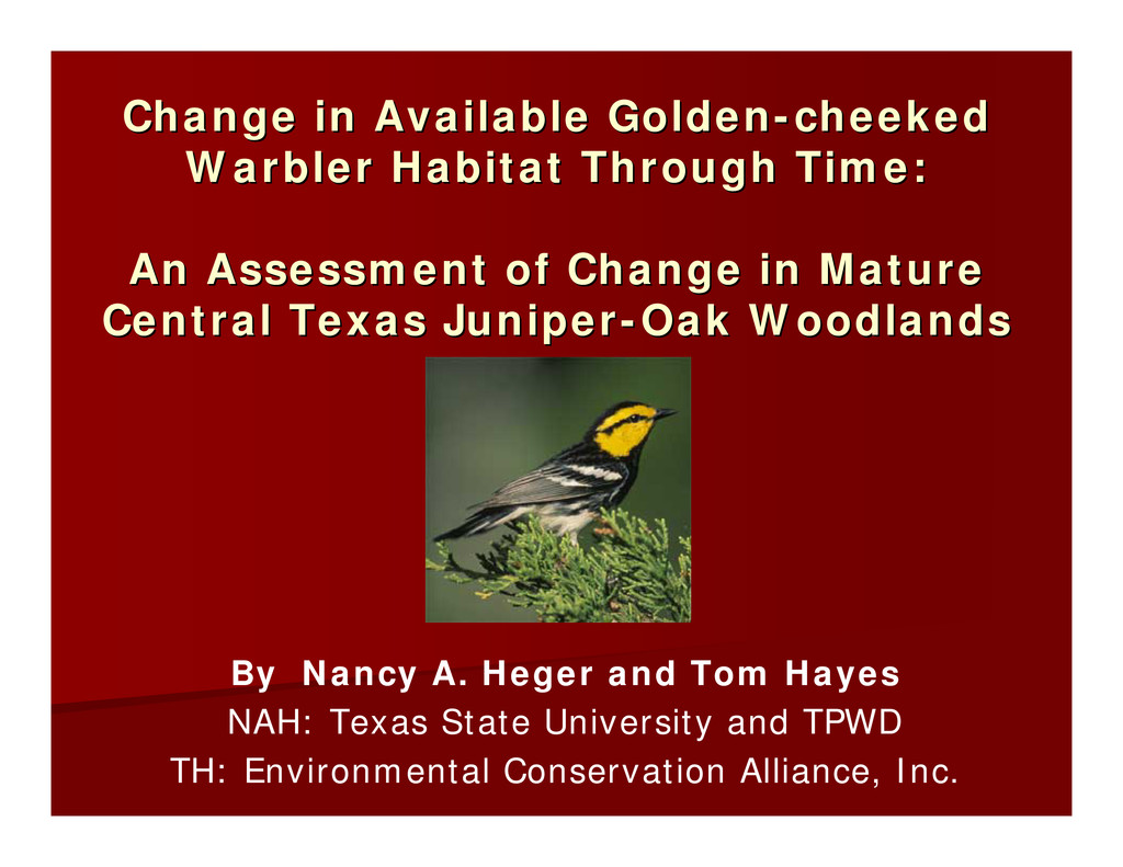
1. Change in Available Golden Change in Available Golden- -cheeked cheeked Warbler Habitat Through Time: Warbler Habitat Through Time: An Assessment of Change in Mature An Assessment of Change in Mature Central Texas Juniper Central Texas Juniper- -Oak Woodlands Oak Woodlands By Nancy A. Heger and Tom Hayes NAH: Texas State University and TPWD TH: Environmental Conservation Alliance, Inc.
2. Golden Golden- -cheeked Warblers (GCWA) cheeked Warblers (GCWA) Setophaga chrysoparia Setophaga chrysoparia (Dendroica chrysoparia)  Prominent golden-cheeks  Females & juveniles less showy than males  Nest only in Central Texas; Texas Hill Country (THC)  Winter in Mexico and Central America Male Female
3. Data Sources: Pulich 1976, USFWS 1992, 2012, Campbell 2003
4. Problem Problem  Range reductions  Significant GCWA population decline  Loss of prime nesting habitat within Central Texas  Mainly due to human population growth • Development & urban sprawl into the THC • Land clearing • Juniper eradication
5. Citizen Involvement Citizen Involvement  Austin environmentalists for protection of endangered species (ES) habitat
6. Endangered Species Listing Endangered Species Listing  May 4, 1990: Emergency rule to place GCWA on the endangered species list  Still, development and growth continues especially in the THC west of Austin  Balcones Canyonlands Conservation Plan (BCCP) • creation of a 30,428 acre preserve system in Travis County (Balcones Canyonlands Preserve (BCP))
7. Previous Assessments and Previous Assessments and Current Needs Current Needs  Previous Research: single time-point estimations of population numbers and available habitat  Trends in loss or gain of habitat have not been documented through time  We used remote sensing and GIS to assess GCWA habitat change from 1986 to 2005 (later add 2010)
8. Significance Significance  Need to restore GCWA populations  Information on gains and losses helps to • Access where to focus effort • Access effectiveness of past management  Protecting GCWA also • Protects others species • Protects the Edwards aquifer
9. Modeling GCWA Habitat  Typical Nesting Habitat: Ashe juniper- oak woodland (Mixed habitat)  Only mature junipers (20-30 yrs; 4.5 m tall) produce shredding bark for nesting Prefers  thick canopy  dense forests  large tracts  >100m from edges
10. Study area Study area  We focused on an approximately 3,240,000 ha area surrounding Austin, Travis county Because  Austin – one of the fastest growing areas in the country  Westward urban sprawl & Development  Causes accelerated GCWA habitat loss  Loss is mitigated somewhat by BCCP
11. Study area Study area - - 3,240,000 ha 3,240,000 ha
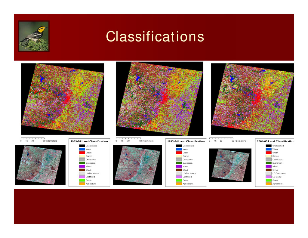
12. Methodology  Select summer & winter TM satellite images  Conduct supervised classifications of stacked images separately for each decade  Conduct Accuracy analysis  Run 3 GCWA habitat Models  Select best model based on GCWA presence data in BCNWR  Identify gains and losses in GCWA habitat through time
13. Winter Winter Summer Summer
14. Winter Summer Winter Summer Mixed Habitat Mixed Habitat
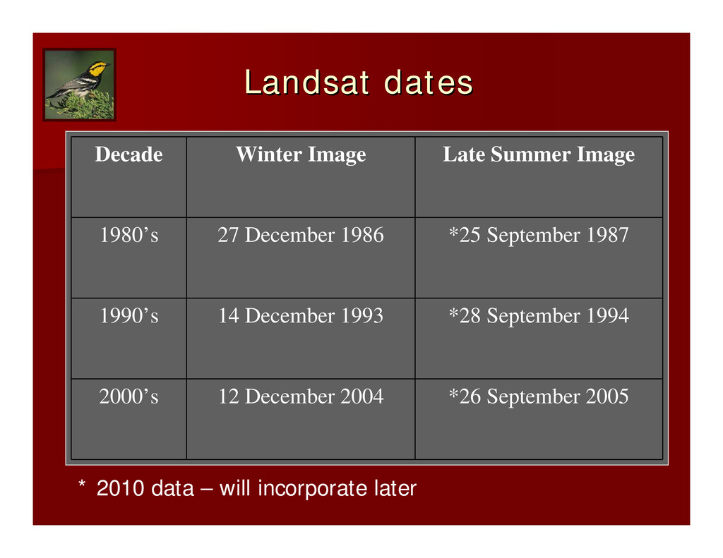
15. Landsat dates Landsat dates Decade Winter Image Late Summer Image 1980’s 27 December 1986 *25 September 1987 1990’s 14 December 1993 *28 September 1994 2000’s 12 December 2004 *26 September 2005 * 2010 data – will incorporate later
16. Land Classes Land Classes Open Water Urban Barren Deciduous forest Evergreen forest Mixed Forest Shrubland Grassland Agriculture
17. Classification  ERDAS Imagine  Stacked summer and winter images  Spectral signatures created; assessed spectral patterns  Supervised classification
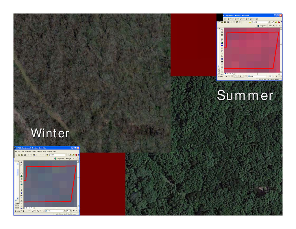
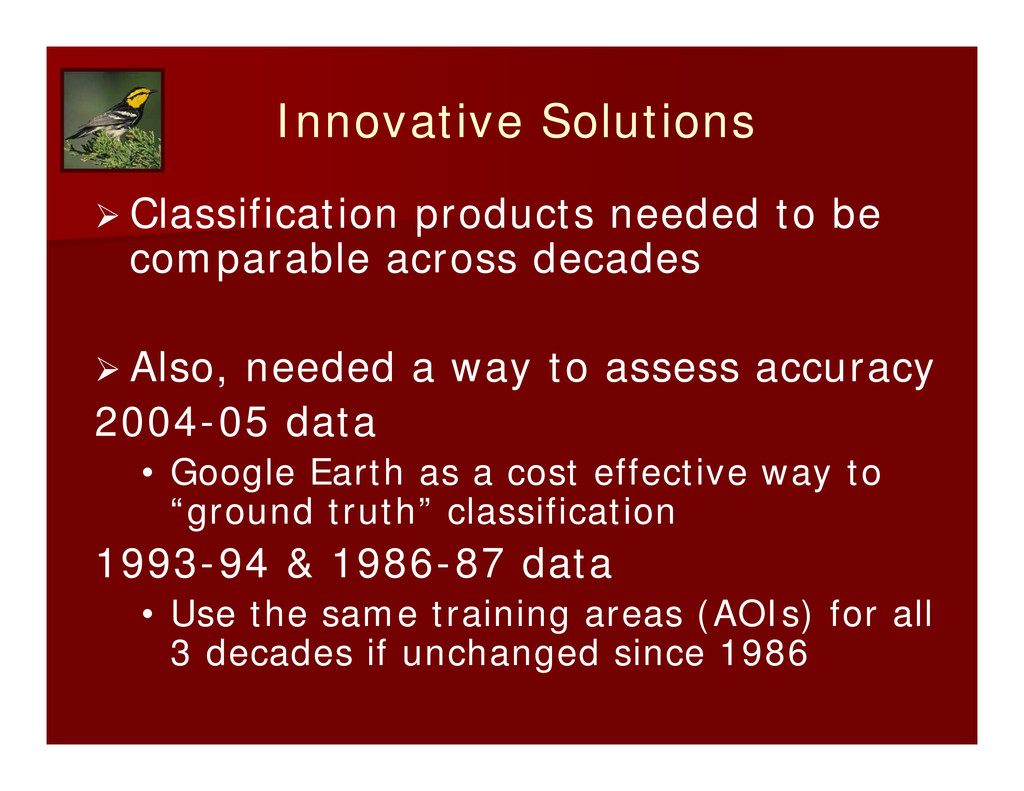
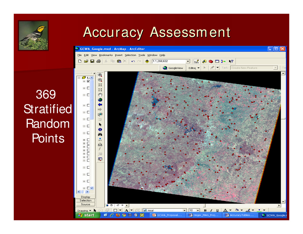
18. Innovative Solutions  Classification products needed to be comparable across decades  Also, needed a way to assess accuracy 2004-05 data • Google Earth as a cost effective way to “ground truth” classification 1993-94 & 1986-87 data • Use the same training areas (AOIs) for all 3 decades if unchanged since 1986
19. Generating AOIs Generating AOIs Agriculture Agriculture
20. 1986 1986 1993 1993 2004 2004 Agriculture Agriculture
21. Mixed Mixed
22. Mixed Habitat Mixed Habitat Winter Summer
23. 1987 1987 Mixed Mixed 1994 1994 2005 2005
24. Classifications
25. Accuracy Assessment Accuracy Assessment 369 Stratified Random Points
26. Accuracy Assessment  Overall Accuracy 87 %; Kappa 85% Class UA OE PA CE Water 100 0 96 4 Urban 76 24 92 8 Barren 100 0 84 16 Deciduous 95 5 79 11 Evergreen 90 10 70 30 Mixed 70 30 84 16 Grass-Shrub 87 13 86 14 Agriculture 79 21 100 0
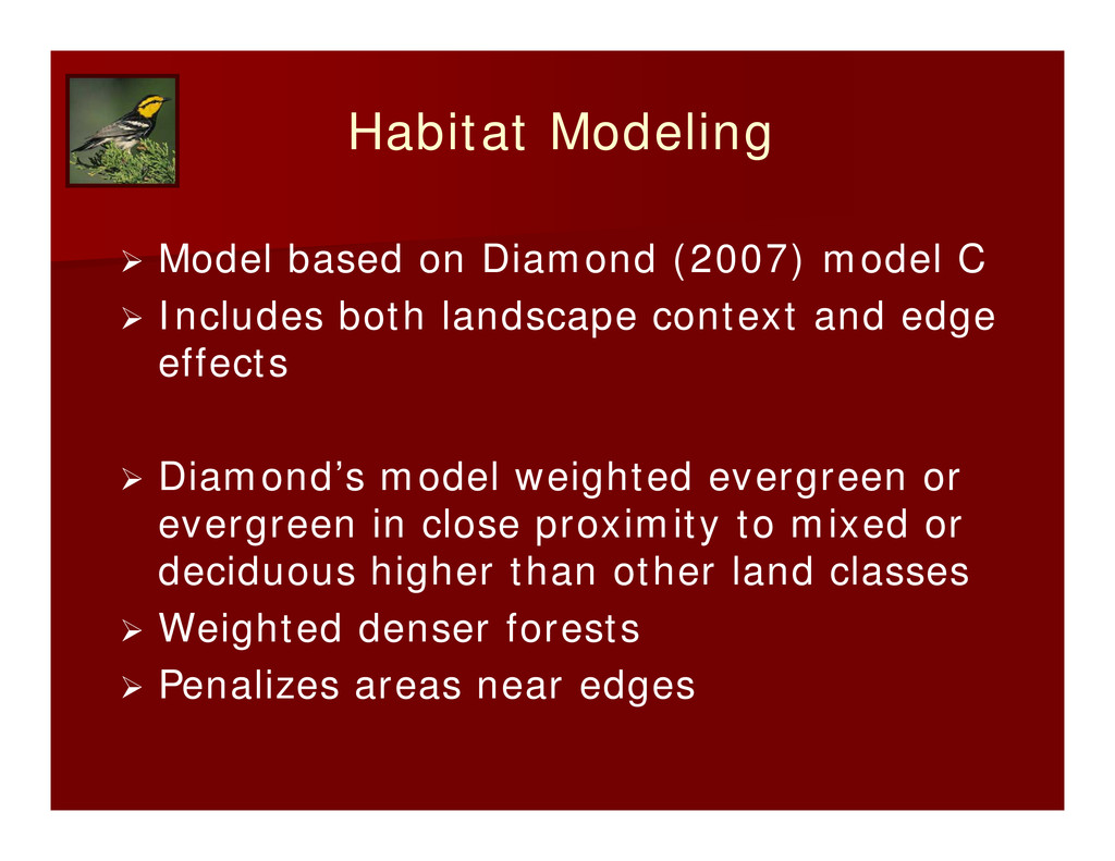
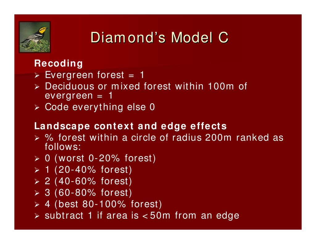
27. Habitat Modeling  Model based on Diamond (2007) model C  Includes both landscape context and edge effects  Diamond’s model weighted evergreen or evergreen in close proximity to mixed or deciduous higher than other land classes  Weighted denser forests  Penalizes areas near edges
28. Diamond Diamond’ ’s Model C s Model C Recoding  Evergreen forest = 1  Deciduous or mixed forest within 100m of evergreen = 1  Code everything else 0 Landscape context and edge effects  % forest within a circle of radius 200m ranked as follows:  0 (worst 0-20% forest)  1 (20-40% forest)  2 (40-60% forest)  3 (60-80% forest)  4 (best 80-100% forest)  subtract 1 if area is <50m from an edge
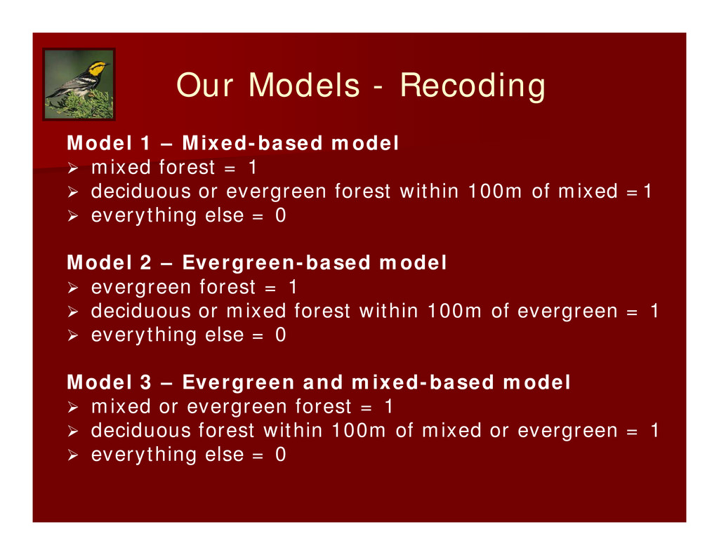
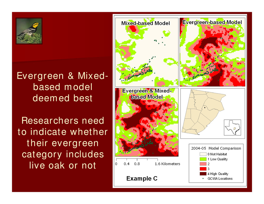
29. Our Models - Recoding Model 1 – Mixed-based model  mixed forest = 1  deciduous or evergreen forest within 100m of mixed =1  everything else = 0 Model 2 – Evergreen-based model  evergreen forest = 1  deciduous or mixed forest within 100m of evergreen = 1  everything else = 0 Model 3 – Evergreen and mixed-based model  mixed or evergreen forest = 1  deciduous forest within 100m of mixed or evergreen = 1  everything else = 0
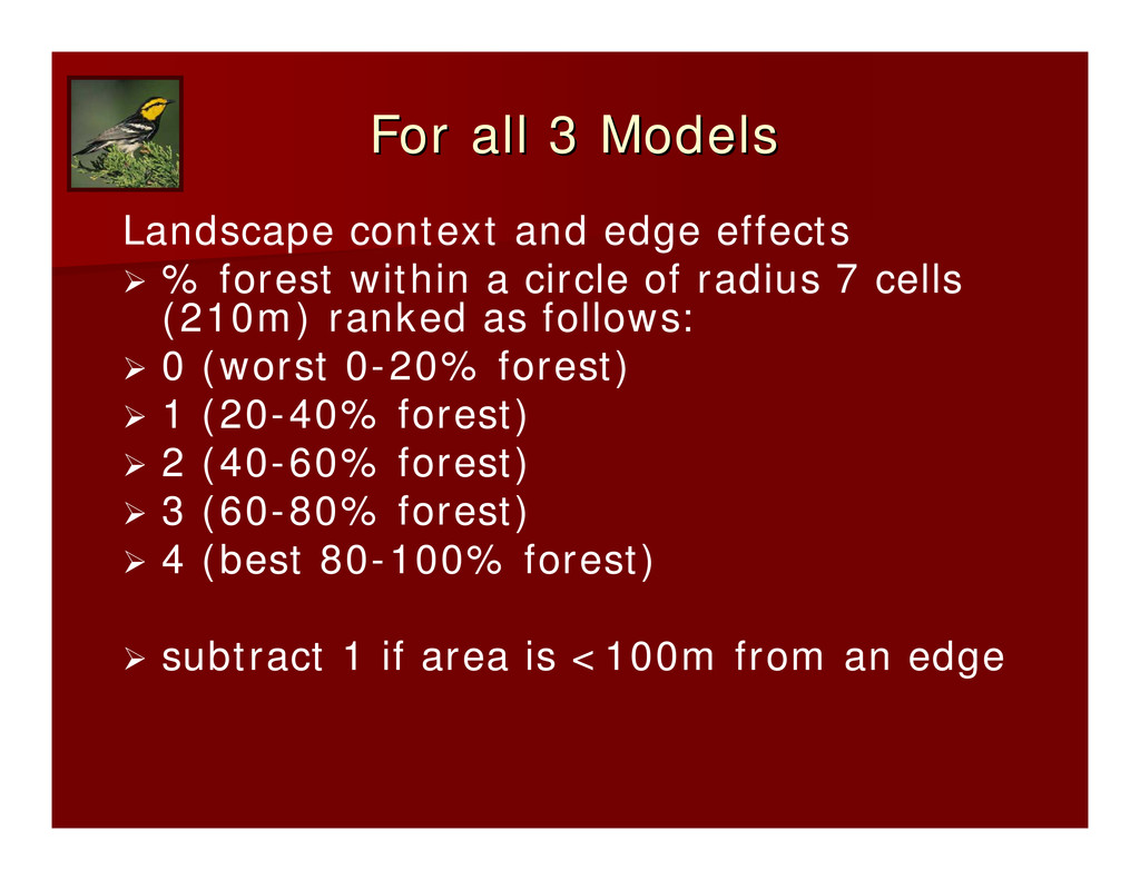
30. For all 3 Models For all 3 Models Landscape context and edge effects  % forest within a circle of radius 7 cells (210m) ranked as follows:  0 (worst 0-20% forest)  1 (20-40% forest)  2 (40-60% forest)  3 (60-80% forest)  4 (best 80-100% forest)  subtract 1 if area is <100m from an edge
31. Model Evaluation  Model predictions were compared to GCWA data  USFWS provided a data set of 2025 GCWA location points in BCNWR from 1993 to 2010  The model coinciding most highly with this data = best model
33. Evergreen & Mixed- based model deemed best Researchers need to indicate whether their evergreen category includes live oak or not
34. Assessing Change 1. Overall percent of each class 2. Change between decades assessed by rank differences (-4 to +4) • Positive indicates gains • Negative indicates losses 3. Change in quality habitats • Recoded ranks 3 and 4 (>60% forest) as 1 • Rest =0 • Calculate differences
35. Model Results Red and Dark red = best quality habitat Red and Dark red = best quality habitat
36. Percent Change  Ranking differ significantly through time (2 = 56.14, df = 8, P<0.001)  Cell Adjusted standardized residuals indicate • Differences due mainly to 1993-94 & 2004-05 • Rank 0 increased from 1993-94 to 2004-05 • Ranks 2, 3, & 4 decreased from 1993-94 to 2004-05 Thus, • Non-GCWA habitat increased through time • Marginal to high quality GCWA habitat decreased through time
37. Change Between Decades
38. Change in Quality Habitat
39. GCWA Habitat Gains in BCNWR
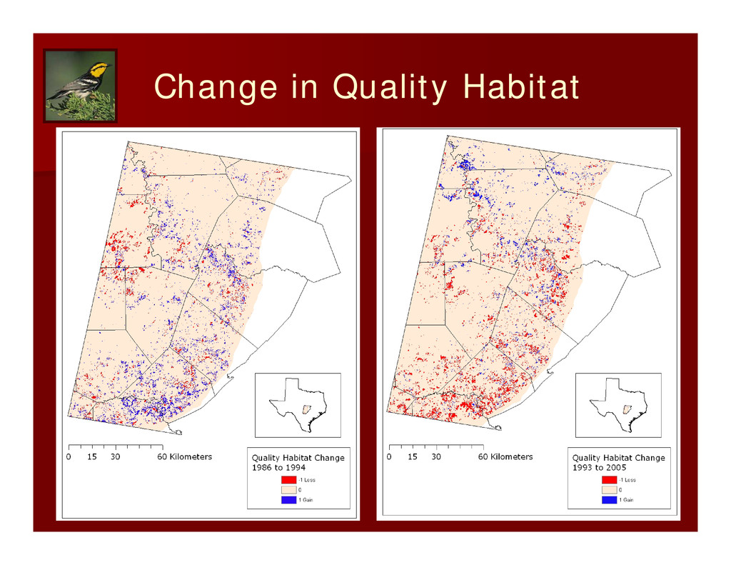
40. Conclusions  Evergreen and mixed-based model best predictor of GCWA habitat  Losses in GCWA habitat have accelerated from 1993-94 to 2004-05  Losses in higher quality GCWA habitat are seen most abundantly near the Austin-San Antonio I-35 corridor  Losses are mitigated somewhat by the BCCP  Even so, losses substantially exceed gains
41. References References DeBoer, T. S. & Diamond, D. D. 2006. Predicting presence-absence of the endangered golden-cheeked warbler (Dendroica chrysoparia). Southwestern Naturalist 51:181-190. Diamond, D. D. 2007. Range-wide modeling of Golden-cheeked warbler habitat. Unpublished report to TPWD. Columbia, Missouri : University of Missouri. Loomis Austin. 2008. Mapping potential golden-cheeked warbler breeding habitat using remotely sensed forest canopy cover data. Report LAI Project No. 051001. Austin, TX: Loomis Austin. Magness, D. R., Wilkins, R. N. & Hejl, S. J. 2006. Quantitative relationships among golden-cheeked warbler occurrence and landscape size, composition, and structure. Wildlife Society Bulletin 34:473-479. Morrison M. L., R. N. Wilkins, B. A. Collier, J. E.Groce, H. A. Mathewson, T. M. McFarland, A. G. Snelgrove, R. T. Snelgrove, and K. L. Skow. 2010. Golden-cheeked warbler population distribution and abundance. College Station, TX: Texas A&M Institute of Renewable Natural Resources. GCWA Photo source: U.S. Fish and Wildlife Service
42. Photo Sources  Title slide Male GCWA – USFWS  Species slide Male GCWA - Rolf Nussbaumer, naturepl.com  Female GCWA - texasgloria52 on flickr.com  Austin Environmentalist – Kim Ludeke, TPWD  Oak-Juniper woodland – TPWD, GIS Lab  Lost Maples, Oak-Juniper – scilogs.com
43. Questions? Questions?
44. Overall Change Detection Overall Change Detection  Subtract the 1985-1986 ranks from the 1993- 1994 ranks resulting in the following scale:  4 (improved by 4 ranks; gain)  3 (improved by 3 ranks; gain)  2 (improved by 2 ranks; gain)  1 (improved by 1 rank; gain)  0 (no change)  -1 (worsened by 1 rank; loss)  -2 (worsened by 2 ranks; loss)  -3 (worsened by 3 ranks; loss)  -4 (worsened by 4 ranks; loss)  Create between decade change map