11/16
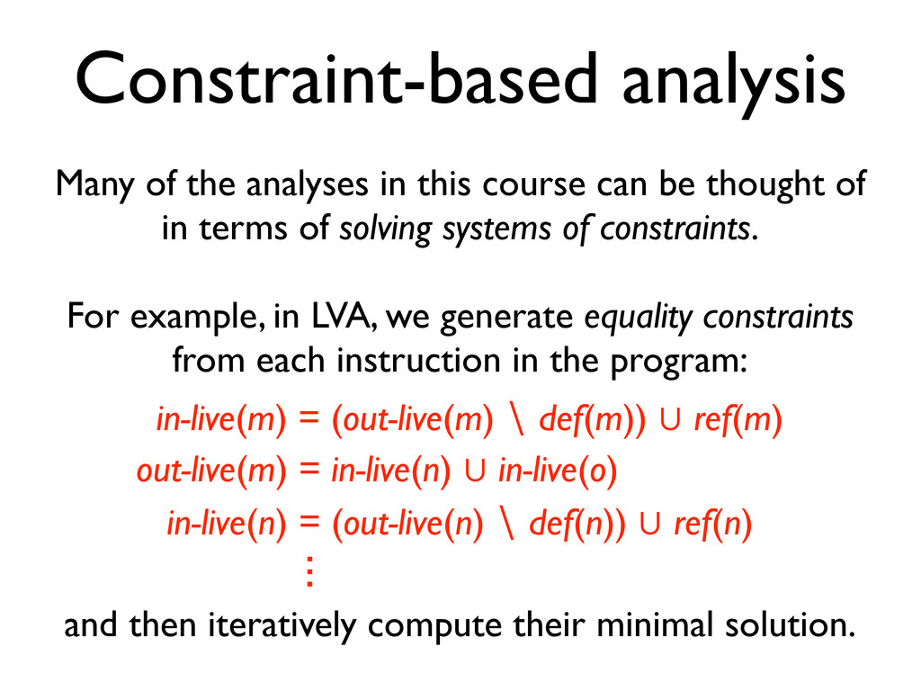
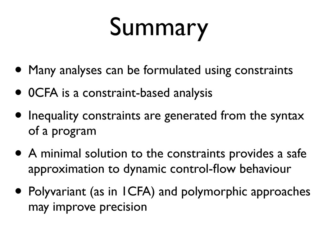
* Many analyses can be formulated using constraints
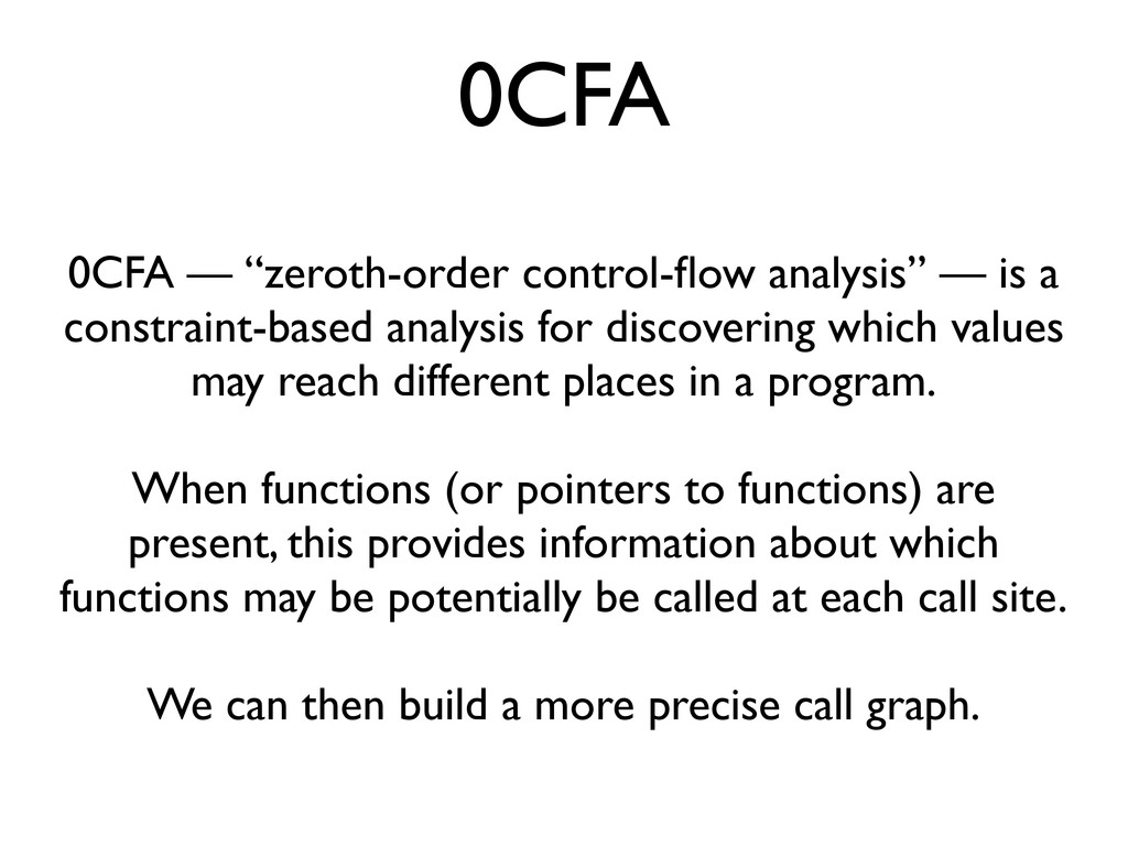
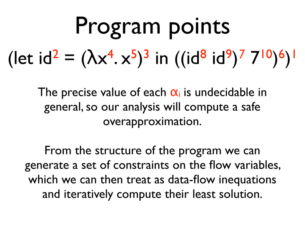
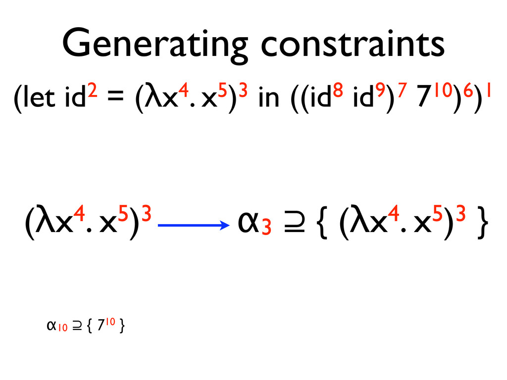
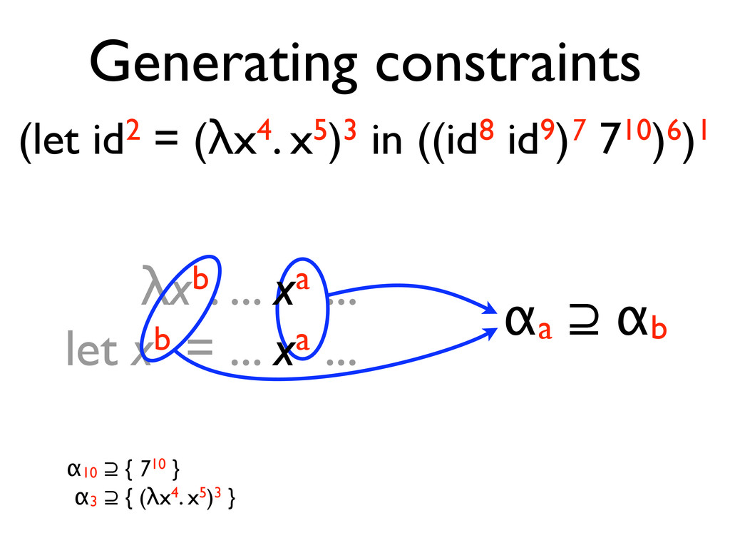
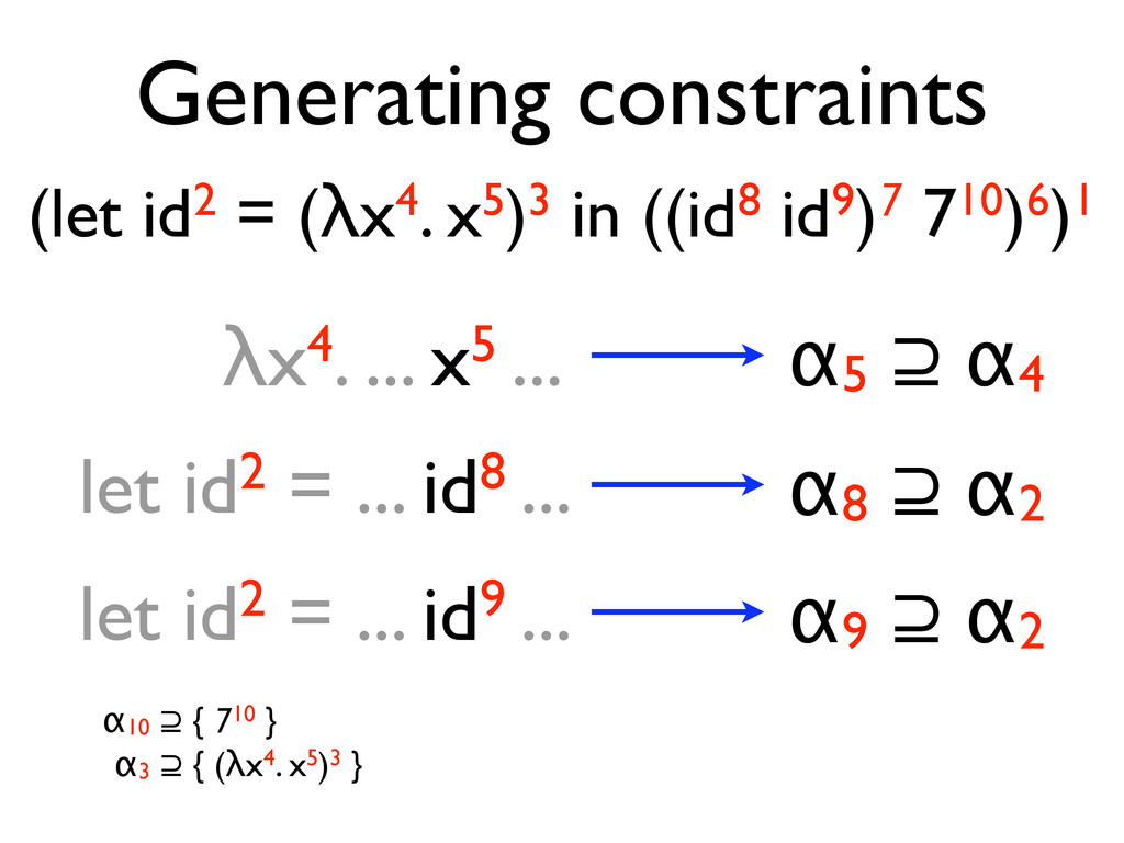
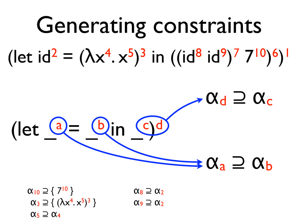
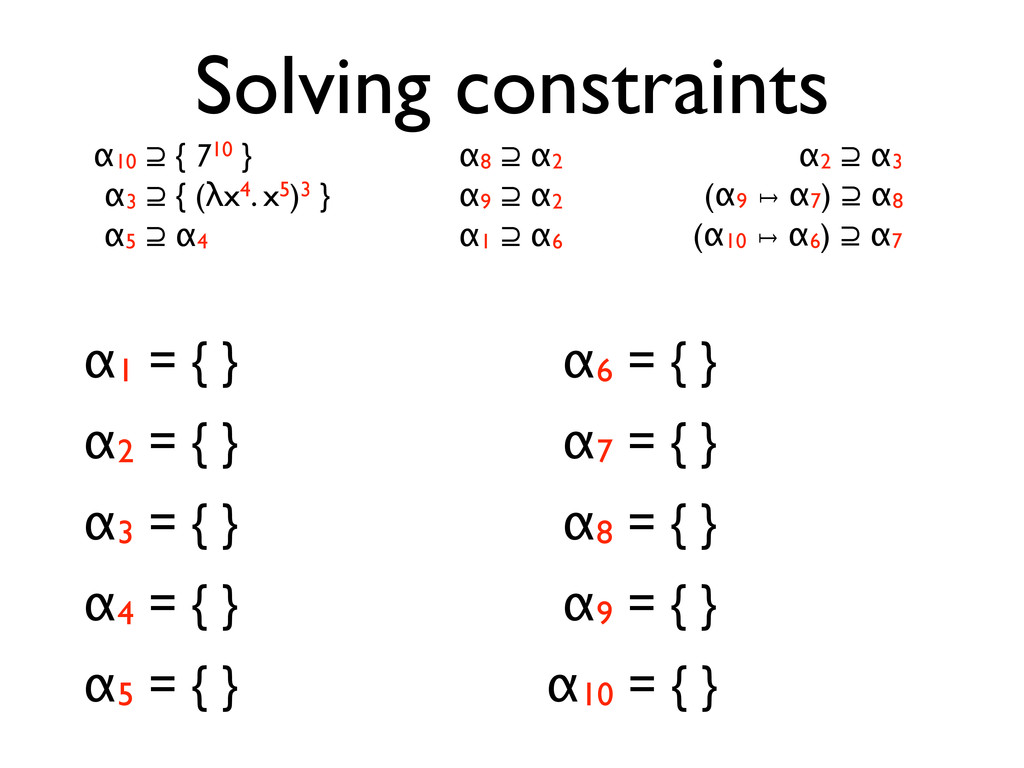
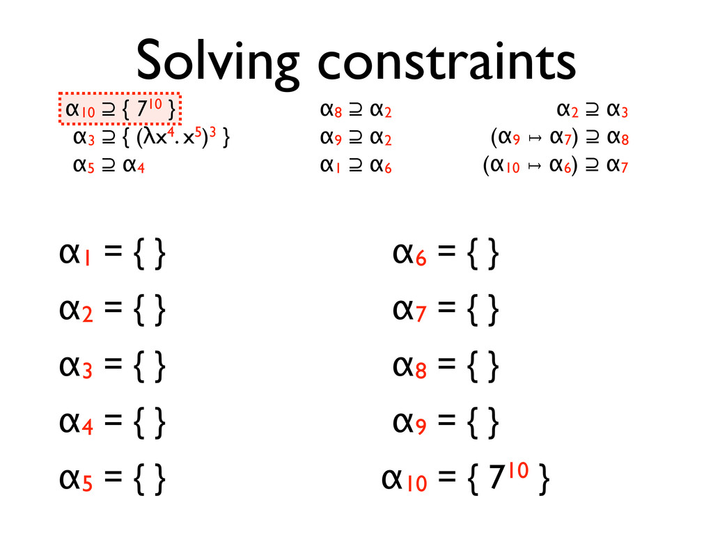
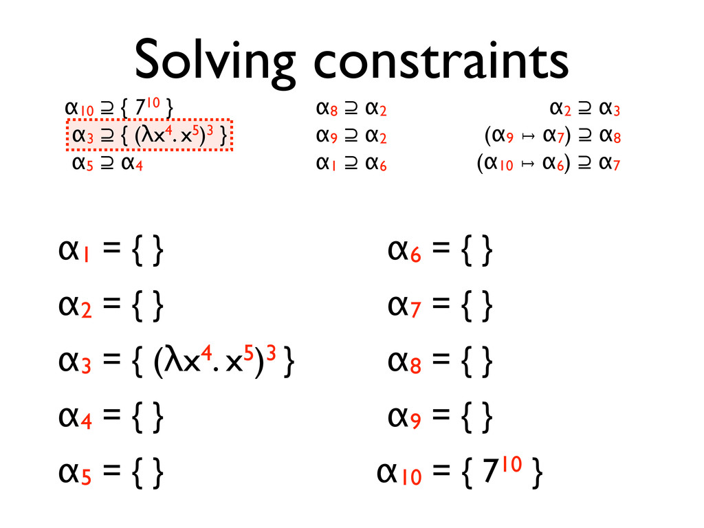
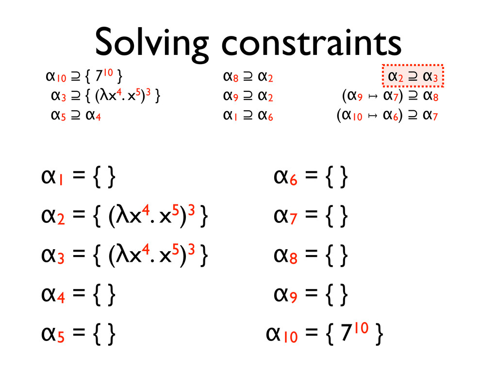
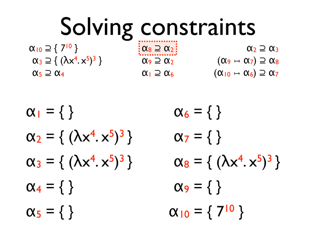
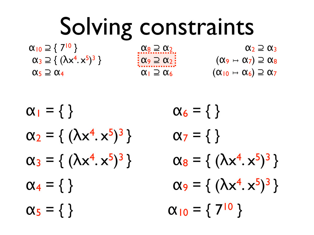
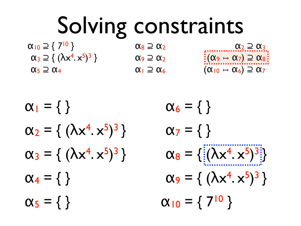
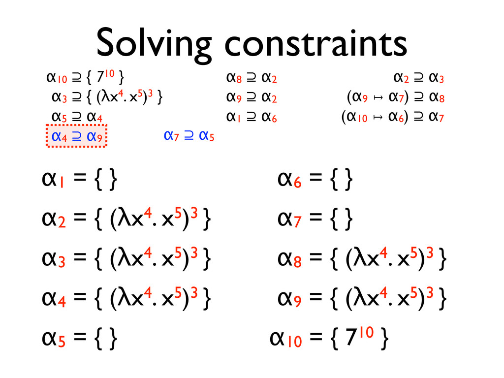
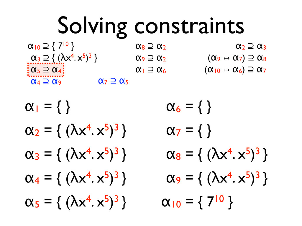
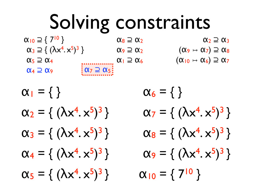
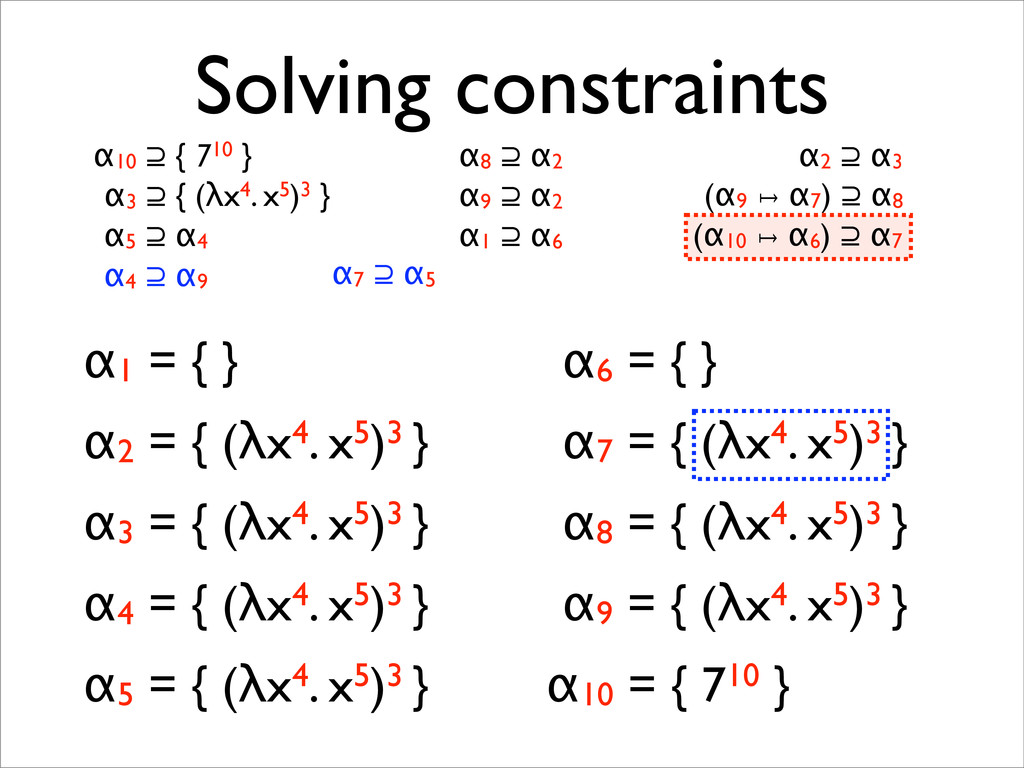
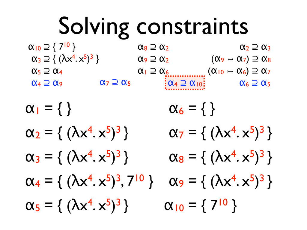
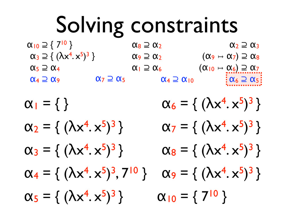
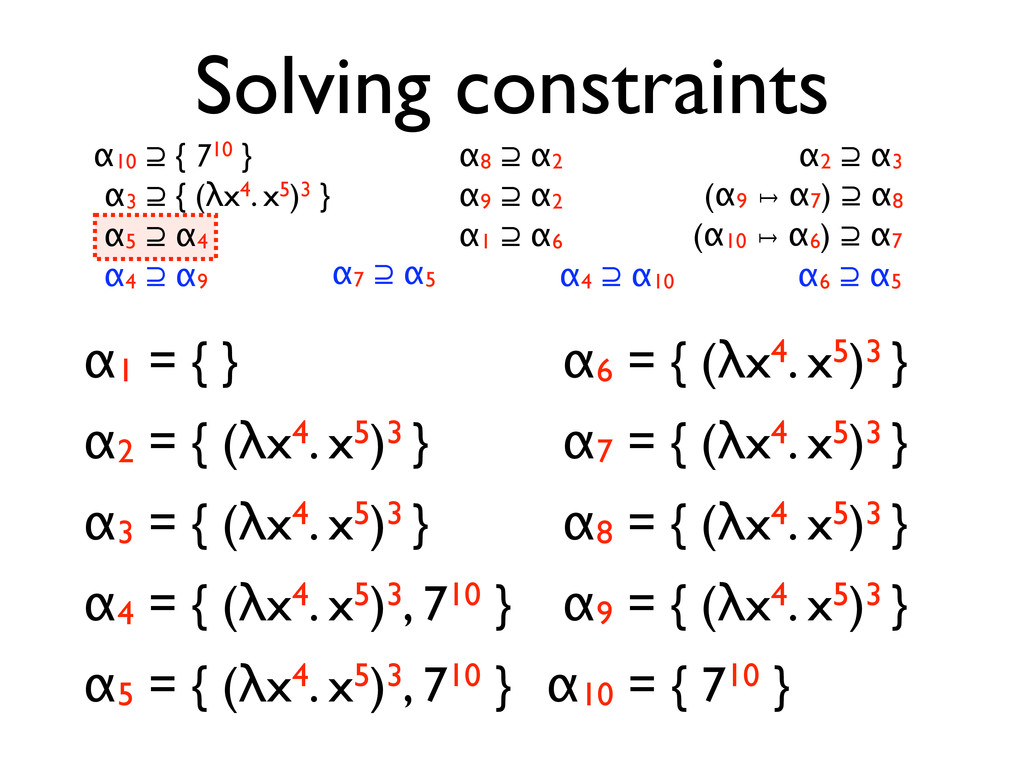
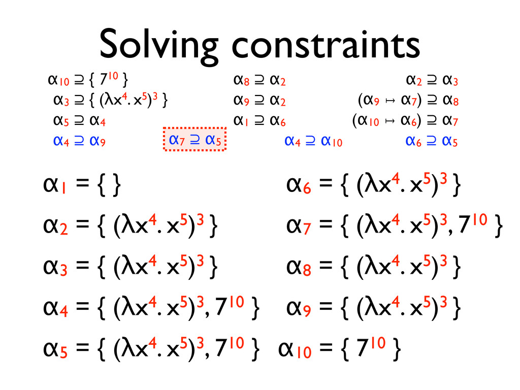
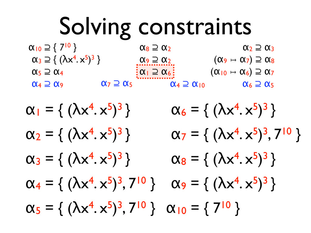
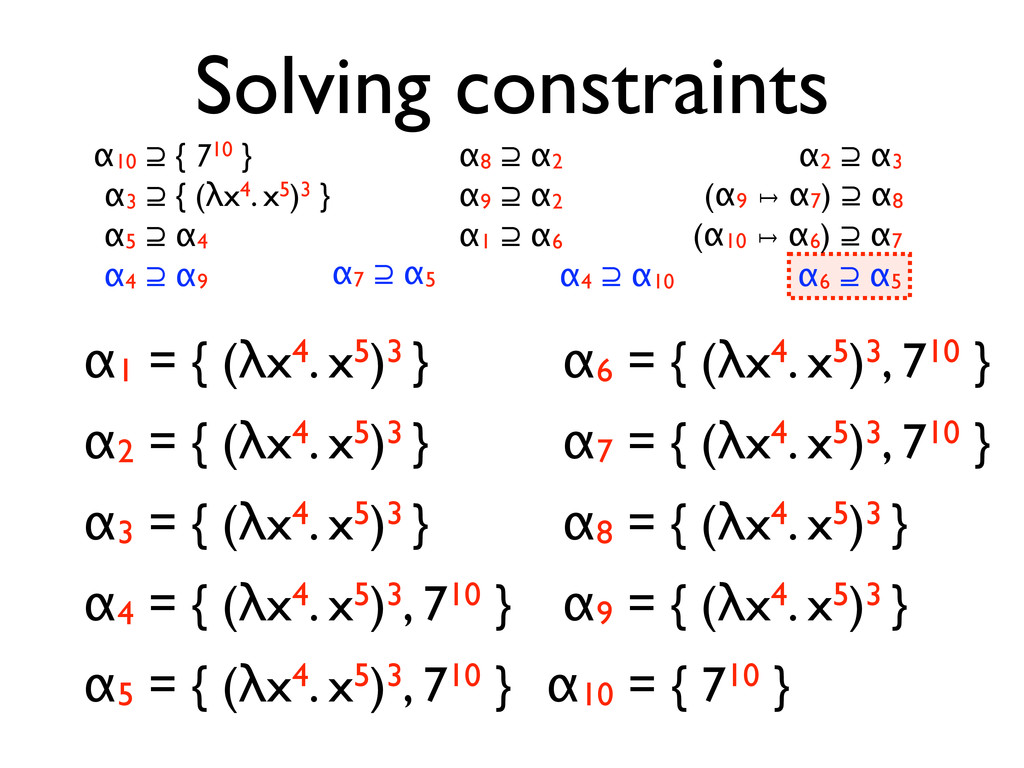
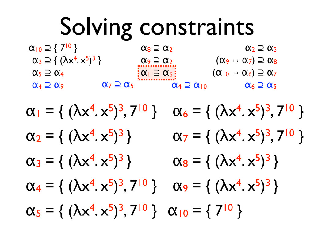
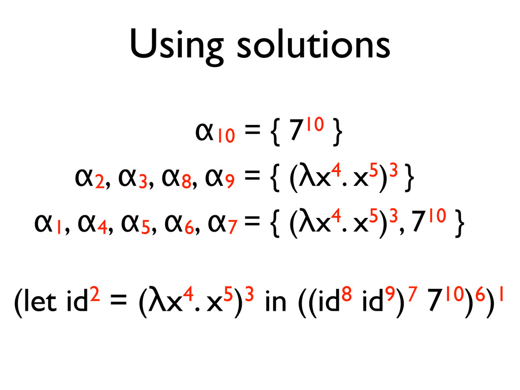
* 0CFA is a constraint-based analysis
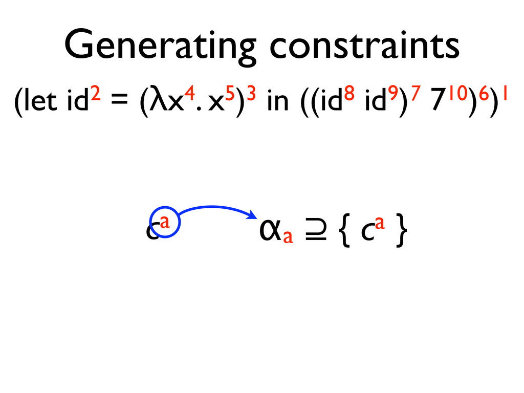
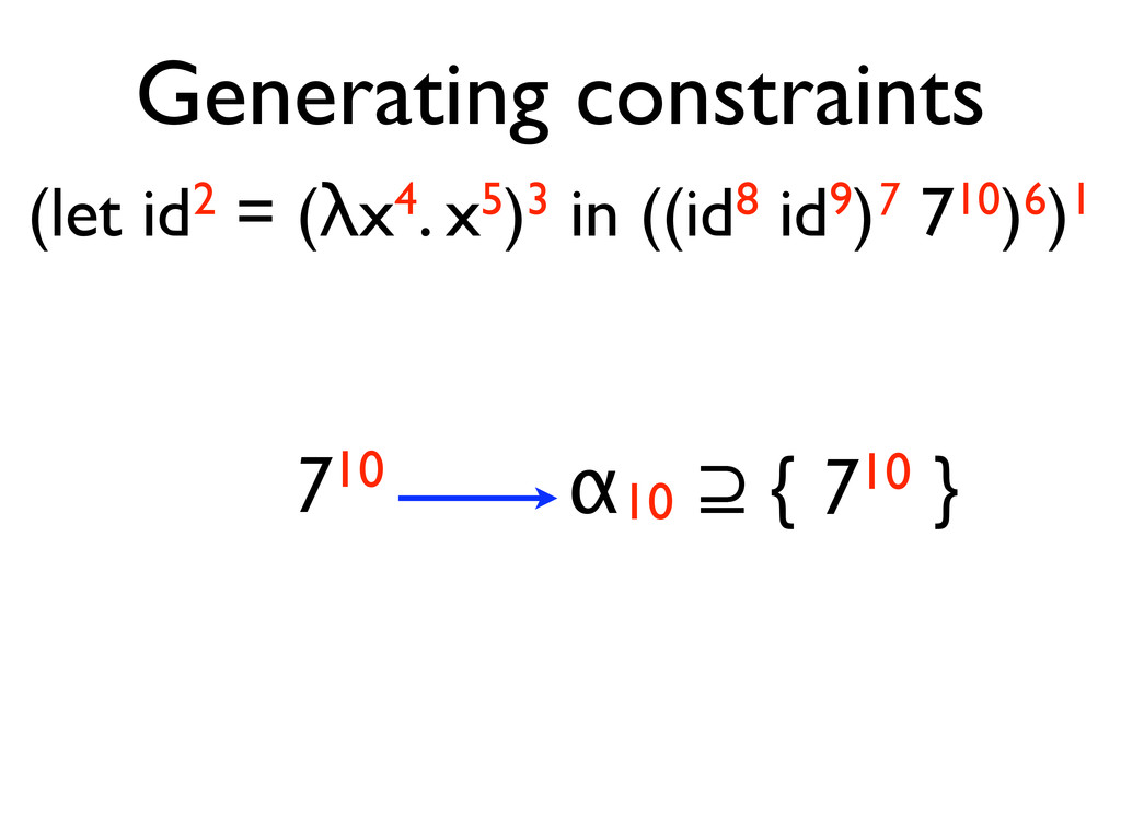
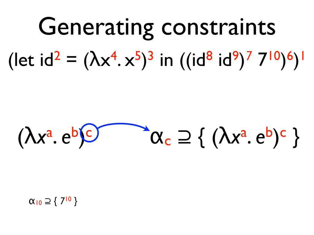
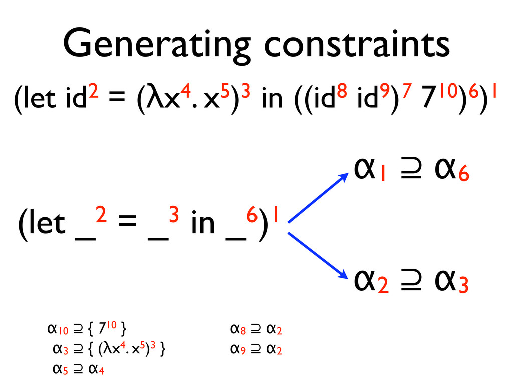
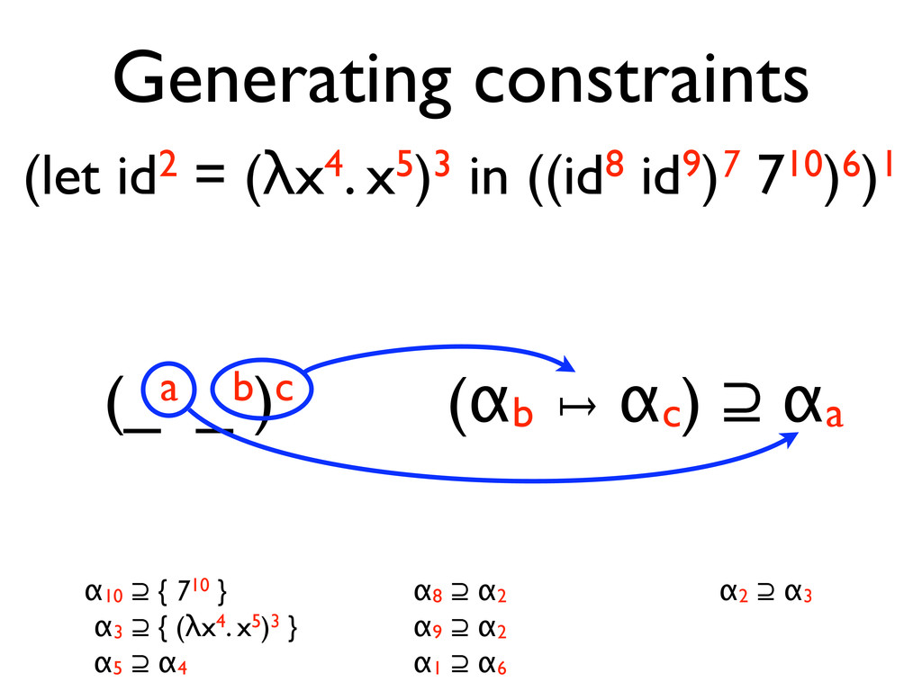
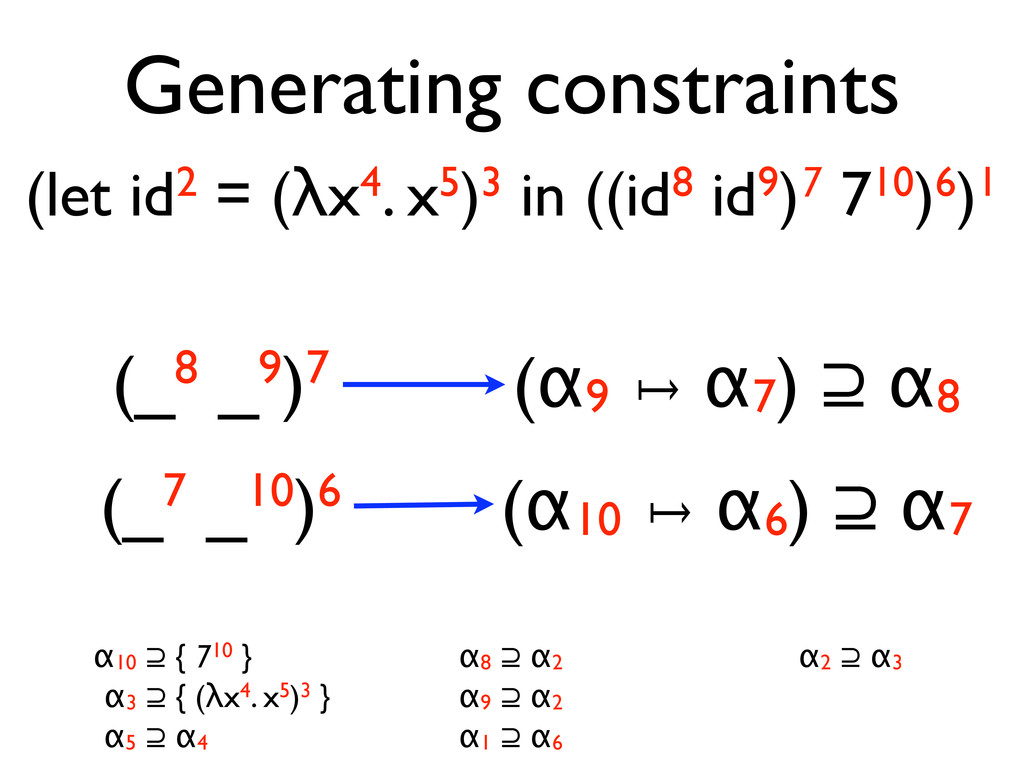
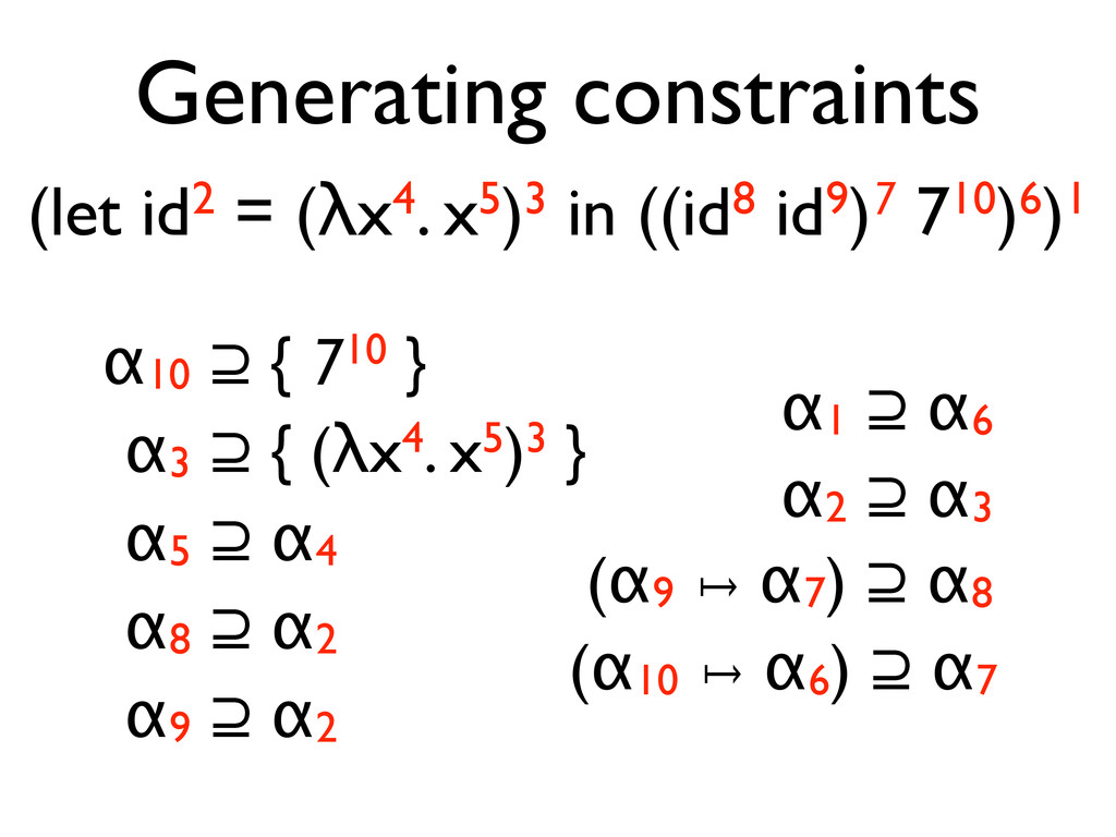
* Inequality constraints are generated from the syntax of a program
* A minimal solution to the constraints provides a safe approximation to dynamic control-flow behaviour
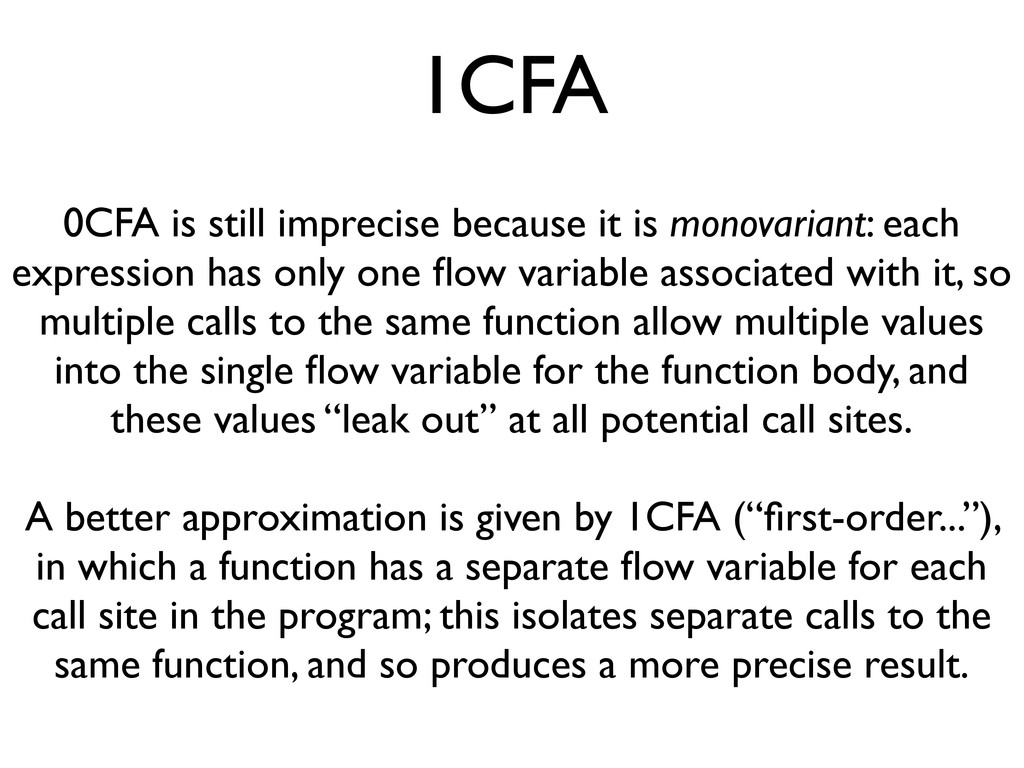
* Polyvariant (as in 1CFA) and polymorphic approaches may improve precision