Calculating Returns to Degree Using Administrative Data

Transcript

1. CALCULATING RETURNS TO DEGREE USING ADMINISTRATIVE DATA TOM SCHENK JR.,

   IOWA DEPARTMENT OF EDUCATION KIYOKAZU MATSUYAMA, IOWA WORKFORCE DEVELOPMENT

2. MOTIVATING QUESTIONS • What are Iowa community colleges role in

   labor supply? • Does a college degree provide economic returns to the individual?

3. ADMINISTRATIVE RECORDS • Educational administrative records rose in popularity during

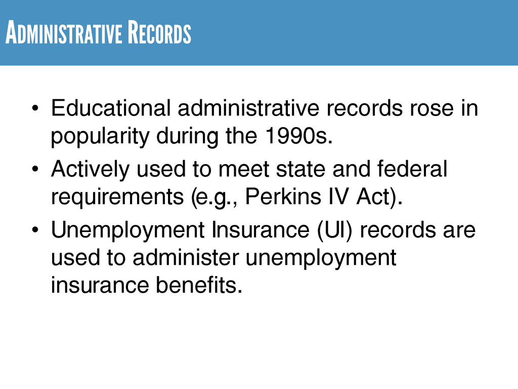
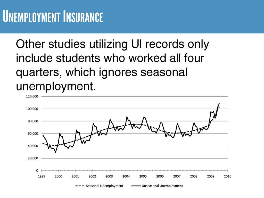
   the 1990s. • Actively used to meet state and federal requirements (e.g., Perkins IV Act). • Unemployment Insurance (UI) records are used to administer unemployment insurance benefits.

4. ADMINISTRATIVE RECORDS & WORKFORCE OUTCOMES • Several studies match educational

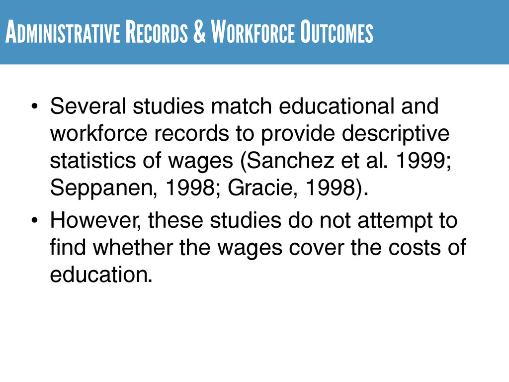
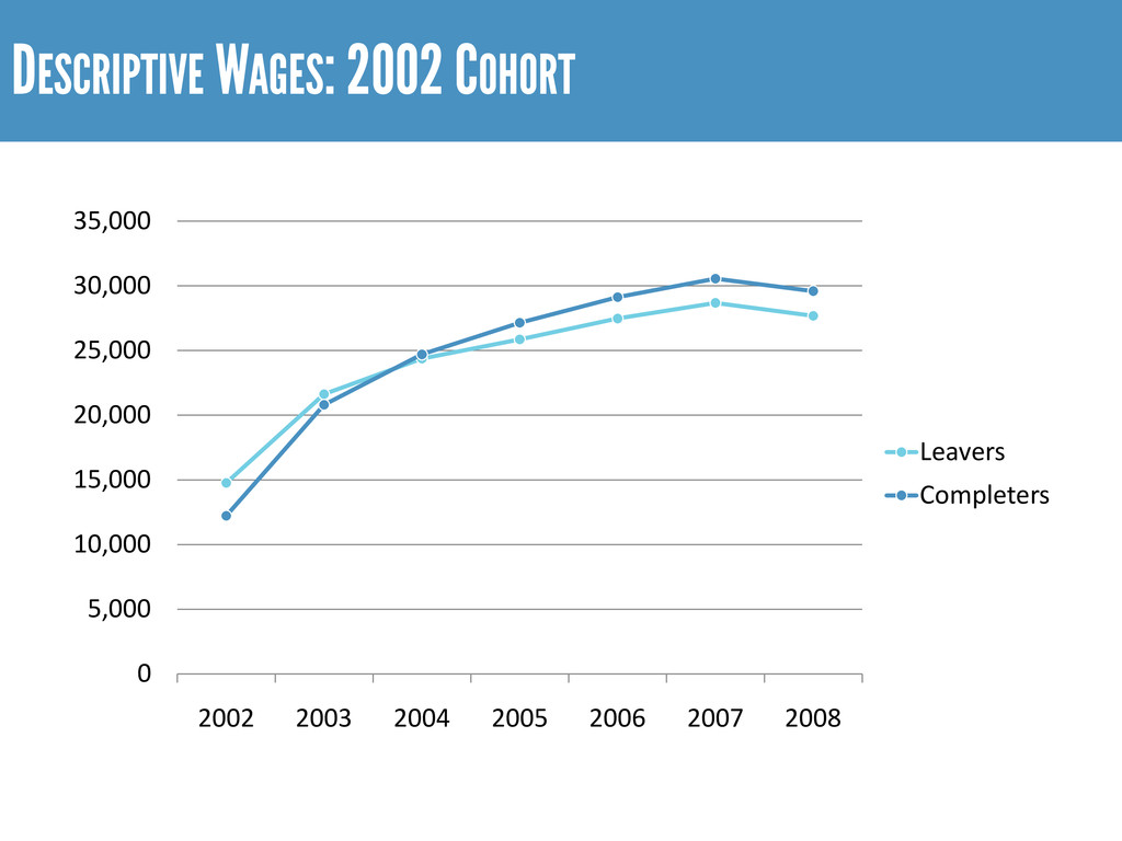
   and workforce records to provide descriptive statistics of wages (Sanchez et al. 1999; Seppanen, 1998; Gracie, 1998). • However, these studies do not attempt to find whether the wages cover the costs of education.

5. TRAINING AND EMPLOYMENT OUTCOMES SYSTEM National Student Clearinghouse Unemployment Insurance

   Community College MIS TEOS

6. STAGGERING COHORTS Leavers Completers 2001 2002 2003 …

7. UNEMPLOYMENT INSURANCE Other studies utilizing UI records only include students

   who worked all four quarters, which ignores seasonal unemployment. 0 20,000 40,000 60,000 80,000 100,000 120,000 1999 2000 2001 2002 2003 2004 2005 2006 2007 2008 2009 2010 Seasonal Unemployment Unseasonal Unemployment

8. DESCRIPTIVE WAGES: 2002 COHORT 0 5,000 10,000 15,000 20,000 25,000

   30,000 35,000 2002 2003 2004 2005 2006 2007 2008 Leavers Completers

9. RETURNS TO DEGREE • Returns to degree calculations have been

   around since 1964 (Becker). • More popular since 1972 (Mincer). • Literally hundreds of papers today.

10. COSTS OF HIGHER EDUCATION • Direct costs (e.g., tuition) •

    Opportunity costs (e.g., lost wages) • Time costs (e.g., higher wages later in life)

11. RATE OF RETURN FORMULATION Wti - Wtj (1 + i

    )t - C Σ T t=1

12. STRATEGY • Assume an interest rate, i, to find the

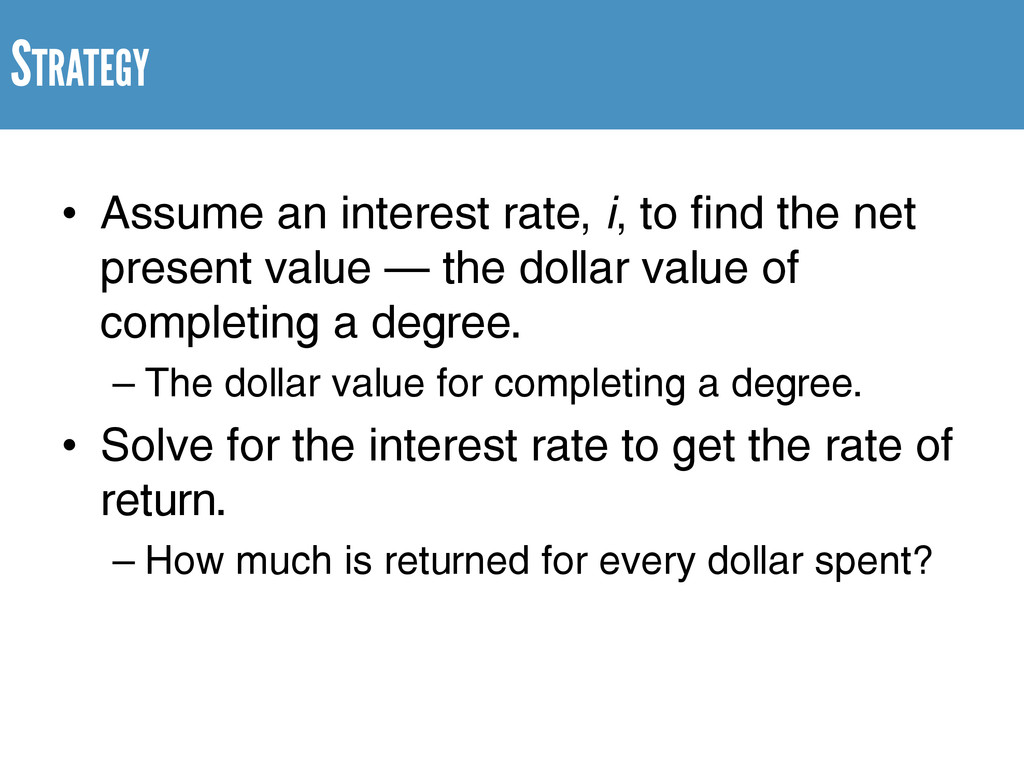
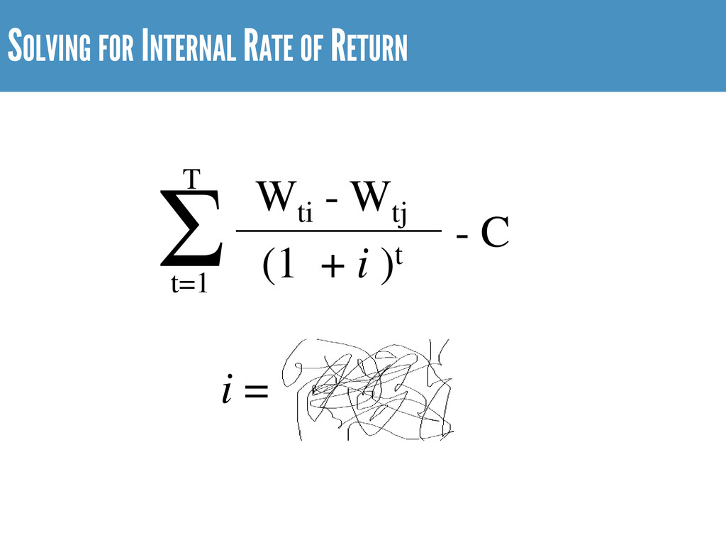
    net present value – the dollar value of completing a degree. – The dollar value for completing a degree. • Solve for the interest rate to get the rate of return. – How much is returned for every dollar spent?

13. NET PRESENT VALUE BY COMPLETION STATUS -20,000 -10,000 0 10,000

    20,000 30,000 40,000 50,000 Completers AA AS AGS AAS Diploma Other

14. POLICY INTERPRETATION FOR NET PRESENT VALUE • NPV for Completers:

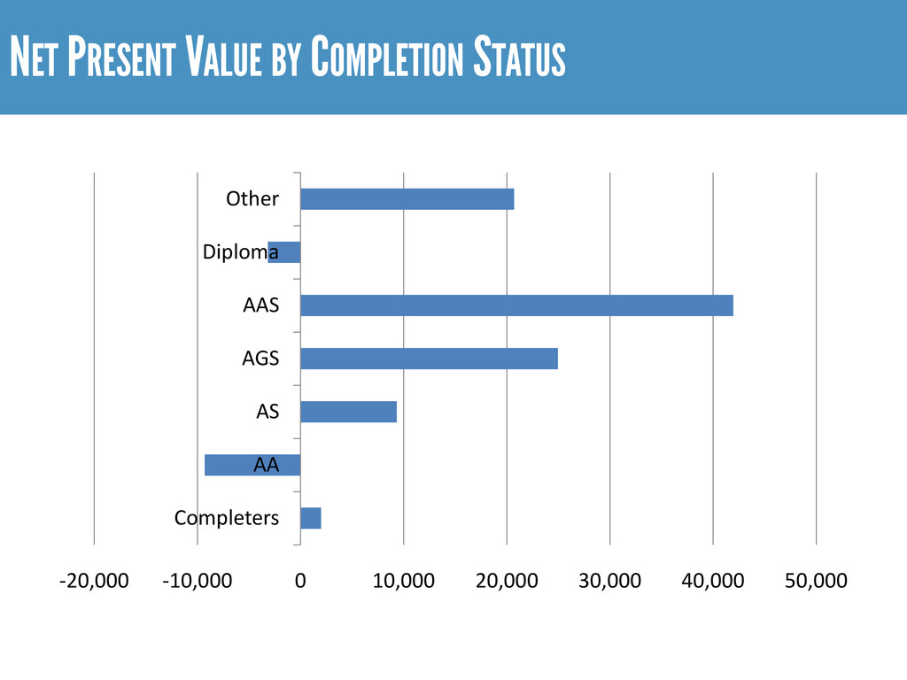
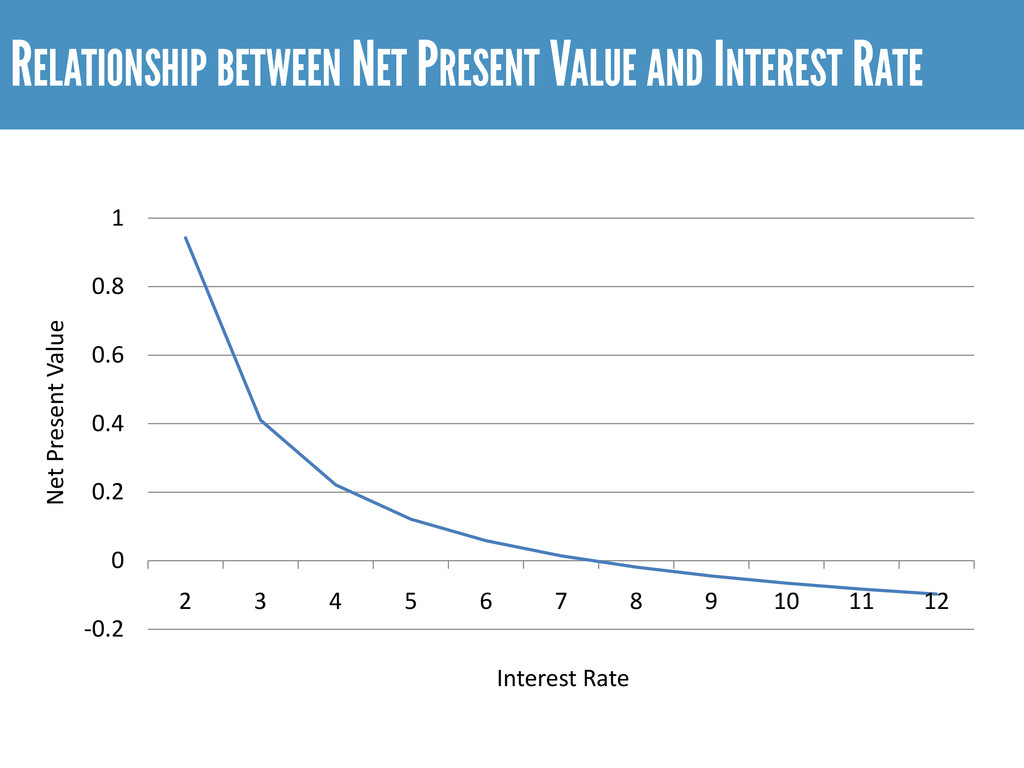
    $1,934 • How much money will it take to convince students to leave community college and enter the workforce? NPV! • NPV for AA recipients: $-9,286. • How much money will it take to convince students to remain in school? NPV! • NPV is the compensation differential.

15. SOLVING FOR INTERNAL RATE OF RETURN Wti - Wtj (1

    + i )t - C Σ T t=1 i =

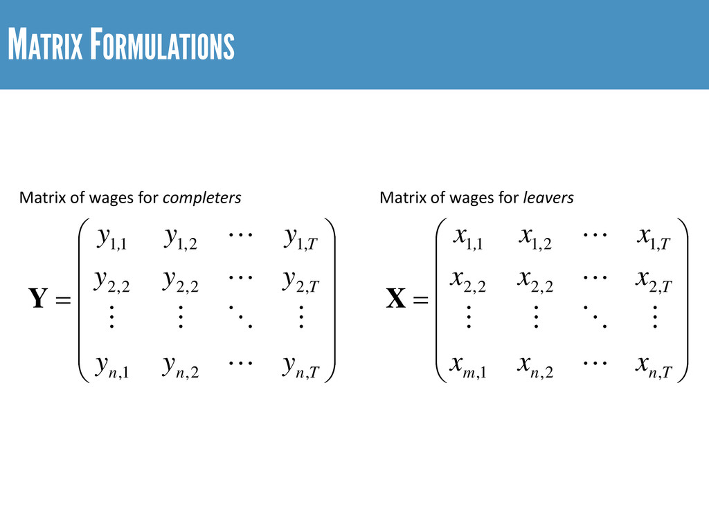
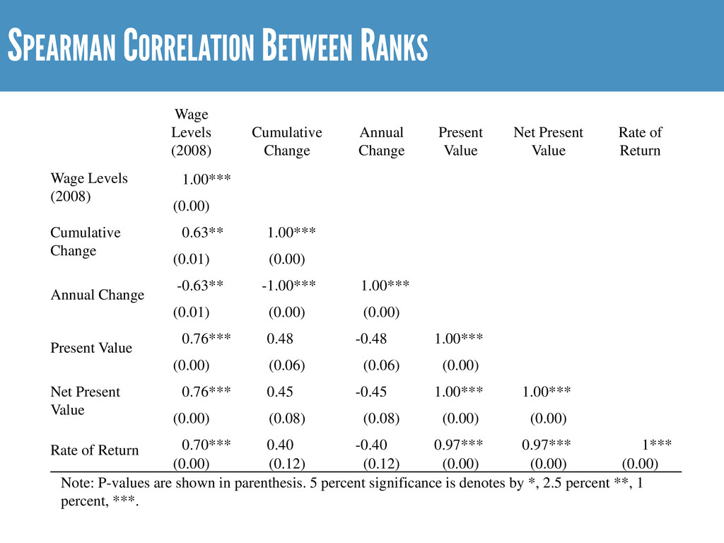
16. MATRIX FORMULATIONS        

          =               = T n n m T T , T n n n T T , x x x x x x x x x y y y y y y y y y , 2 , 1 , , 2 2 , 2 2 , 2 , 1 2 , 1 1 1 , 2 , 1 , , 2 2 , 2 2 , 2 , 1 2 , 1 1 1               X Y Matrix of wages for completers Matrix of wages for leavers

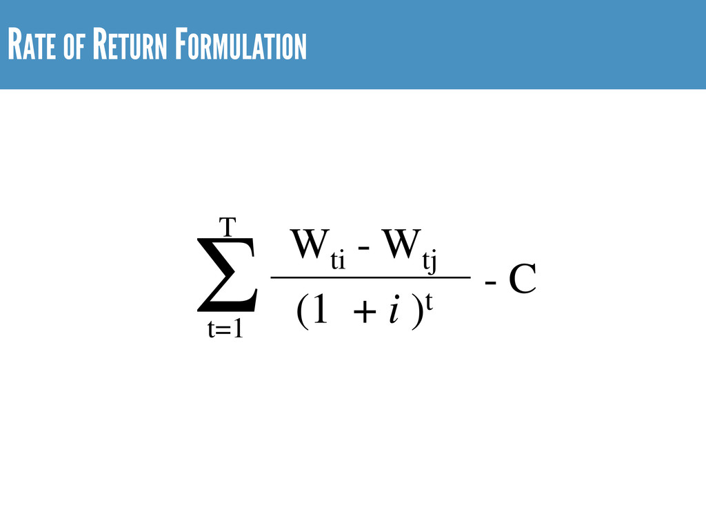
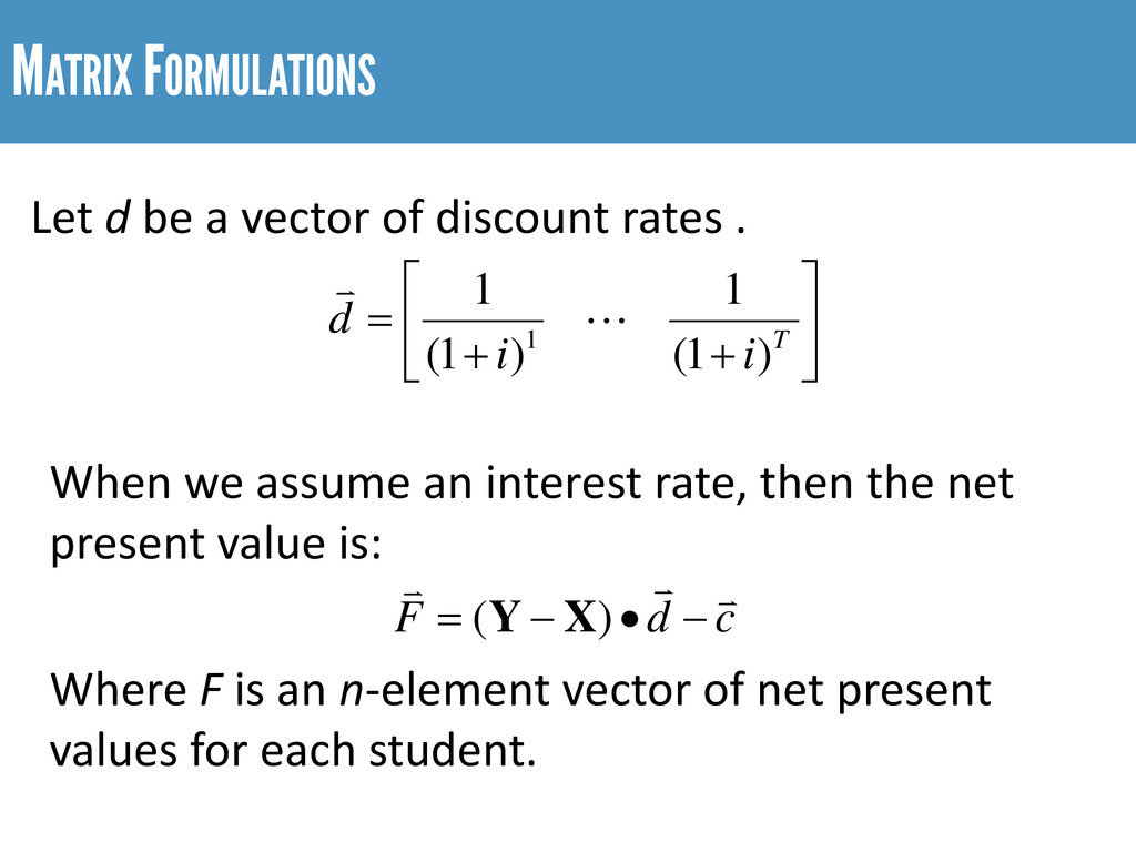
17. MATRIX FORMULATIONS       + +

    = T i i d ) 1 ( 1 ) 1 ( 1 1   Let d be a vector of discount rates . When we assume an interest rate, then the net present value is: c d F    − • − = ) ( X Y Where F is an n-element vector of net present values for each student.

18. RELATIONSHIP BETWEEN NET PRESENT VALUE AND INTEREST RATE -0.2 0

    0.2 0.4 0.6 0.8 1 2 3 4 5 6 7 8 9 10 11 12 Interest Rate Net Present Value

19. NEWTON-RHAPSON MULTIPLE ITERATION Let      

            ∂ ∂ ∂ ∂ = i f i f r J n   1 ) ( 0 ) 1 ( ) ( 1 = − + − = ∑ = c i X Y r f T t t j j so the Jacobian is:

20. NEWTON-RHAPSON MULTIPLE ITERATION Find an a0 so F(a0 ) =

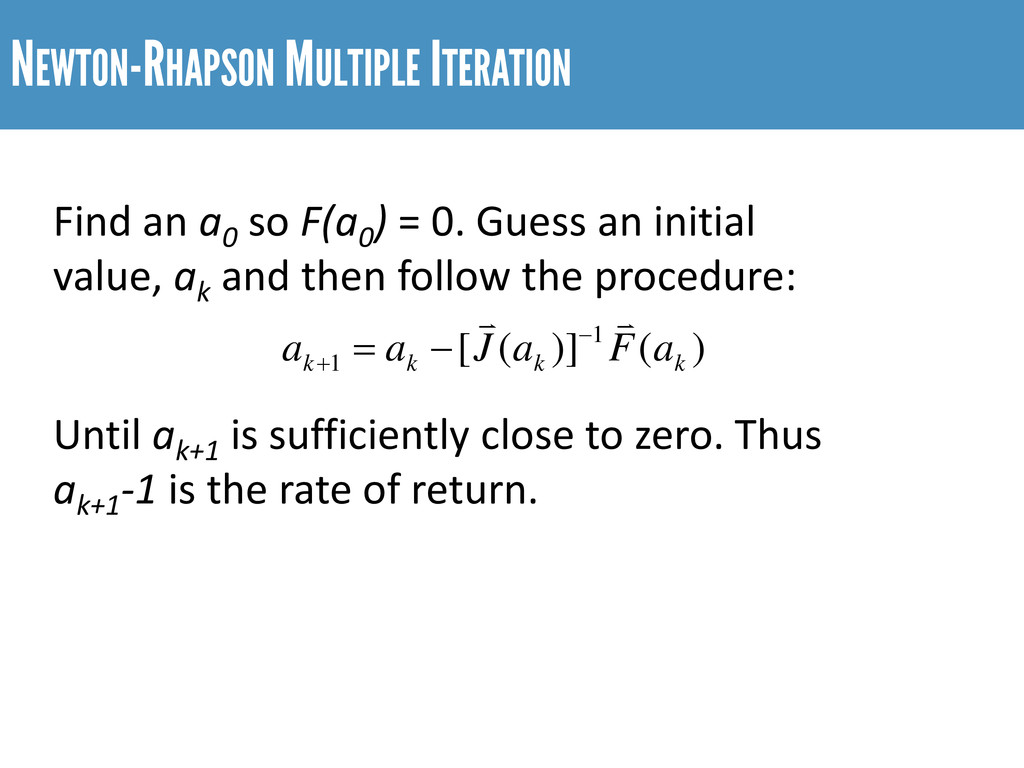
    0. Guess an initial value, ak and then follow the procedure: ) ( )] ( [ 1 1 k k k k a F a J a a   − + − = Until ak+1 is sufficiently close to zero. Thus ak+1 -1 is the rate of return.

21. RETURNS BY AWARD -0.10 0.00 0.10 0.20 0.30 0.40 0.50

    0.60 Completers AA AS AGS AAS Diploma Other

22. RETURN BY CAREER CLUSTER -0.30 -0.20 -0.10 0.00 0.10 0.20

    0.30 0.40 0.50 0.60 Agriculture Construction Finance Government Health IT Law Manufacturing Marketing STEM Transportation

23. COMPARING METHODOLOGIES • What matters most about returns by program?

    → Ranks! 2008 Wage Levels Rate of Return 1. Government 2. STEM 3. Manufacturing 4. Finance 5. Transportation 1. Law 2. STEM 3. Finance 4. Manufacturing 5. Health

24. SPEARMAN CORRELATION BETWEEN RANKS Wage Levels (2008) Cumulative Change Annual

    Change Present Value Net Present Value Rate of Return Wage Levels (2008) 1.00*** (0.00) Cumulative Change 0.63** 1.00*** (0.01) (0.00) Annual Change -0.63** -1.00*** 1.00*** (0.01) (0.00) (0.00) Present Value 0.76*** 0.48 -0.48 1.00*** (0.00) (0.06) (0.06) (0.00) Net Present Value 0.76*** 0.45 -0.45 1.00*** 1.00*** (0.00) (0.08) (0.08) (0.00) (0.00) Rate of Return 0.70*** 0.40 -0.40 0.97*** 0.97*** 1*** (0.00) (0.12) (0.12) (0.00) (0.00) (0.00) Note: P-values are shown in parenthesis. 5 percent significance is denotes by *, 2.5 percent **, 1 percent, ***.

25. ESTIMATED NATIONAL RETURNS • Generally, each additional year of education

    returns 10 percent (Card, 1999; Psacharopulos, 1994; Psacharopulos & Patrinos, 2002; etc.) • Community college to High School returns is between 15 and 27 percent (Leigh & Gill, 1997; Kane & Rouse, 1995, 1999).

26. ESTIMATED RETURNS & IOWA’S ESTIMATES • Earning a degree versus

    leaving early returns is between 6 and 14 percent. • Iowa’s estimates show returns of 6 percent. • Still early in a student’s career, 10 to 15 years later will be better estimates.

27. SUMMARY • Net present value provides a single amount which

    can be used to persuade decisions. • Rate of return provides a dollar-free, single value that is nationally and internationally comparable. • These measures lead to distinct differences in the qualitative interpretations.