in Chamonix Mt Blanc, France, from Monday, Jan. 6 to Wed., Jan. 8 (and BNP workshop on Jan. 9), 2014 All aspects of MCMC++ theory and methodology and applications and more! All posters welcomed! Website http://www.pages.drexel.edu/∼mwl25/mcmski/
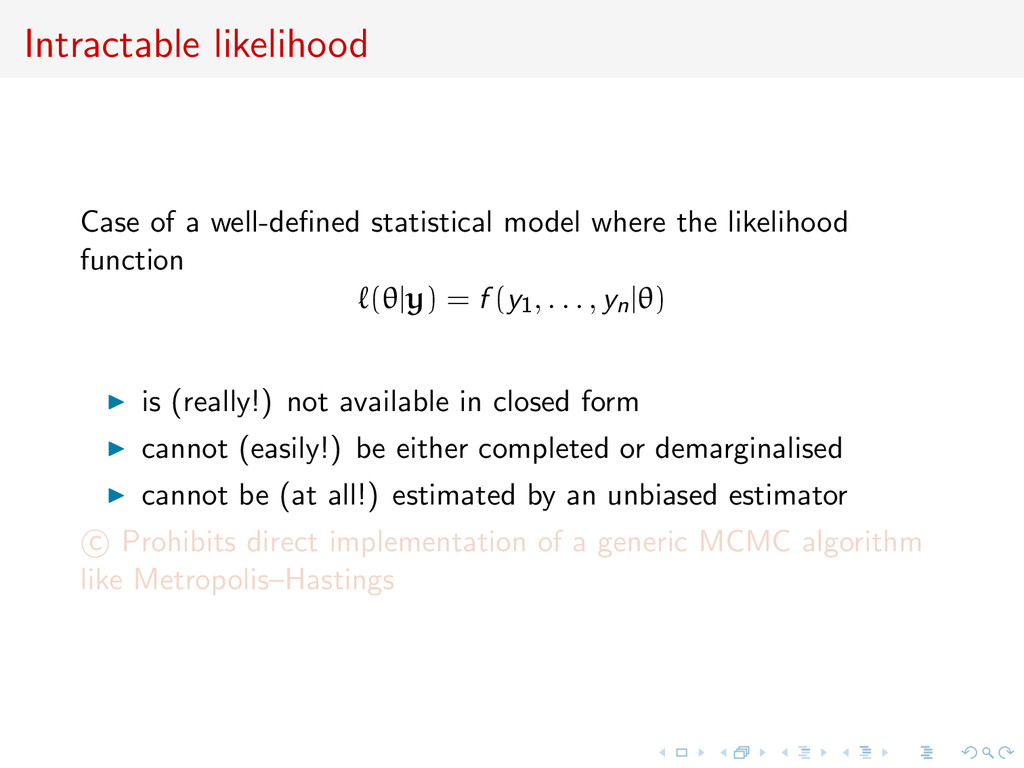
likelihood function (θ|y) = f (y1, . . . , yn|θ) is (really!) not available in closed form cannot (easily!) be either completed or demarginalised cannot be (at all!) estimated by an unbiased estimator c Prohibits direct implementation of a generic MCMC algorithm like Metropolis–Hastings
likelihood function (θ|y) = f (y1, . . . , yn|θ) is (really!) not available in closed form cannot (easily!) be either completed or demarginalised cannot be (at all!) estimated by an unbiased estimator c Prohibits direct implementation of a generic MCMC algorithm like Metropolis–Hastings
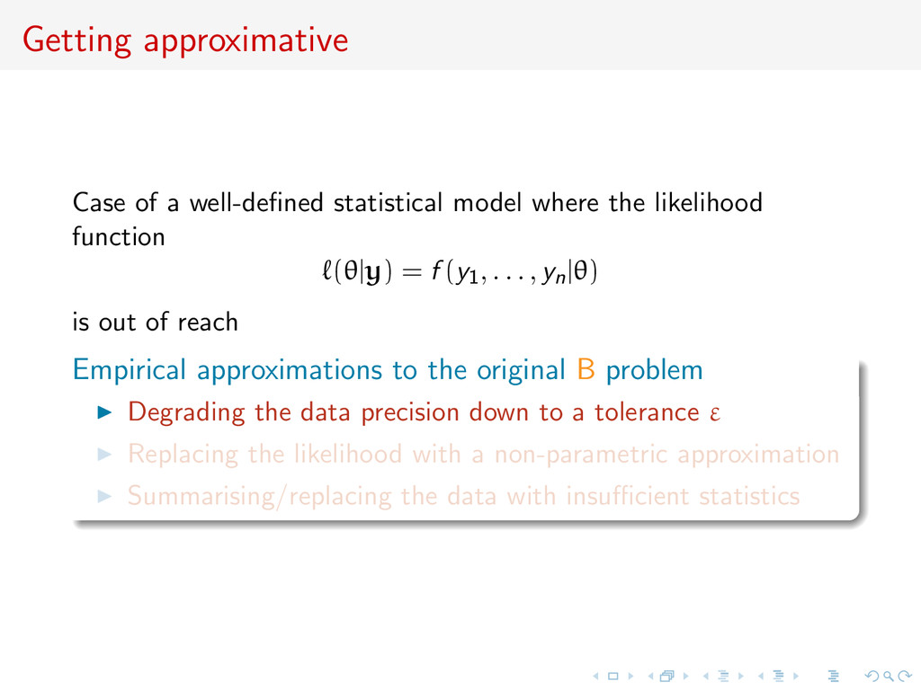
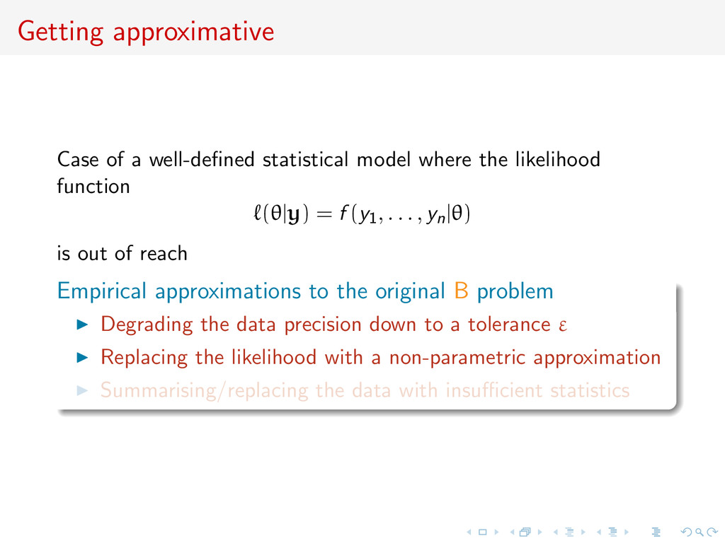
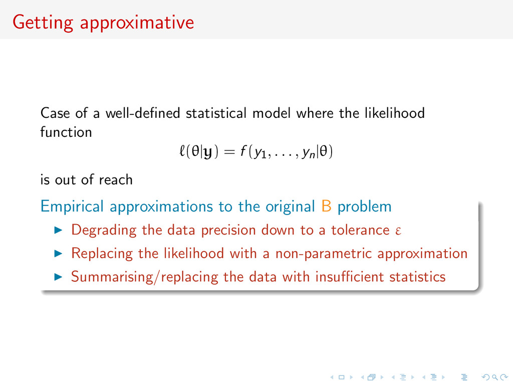
likelihood function (θ|y) = f (y1, . . . , yn|θ) is out of reach Empirical approximations to the original B problem Degrading the data precision down to a tolerance ε Replacing the likelihood with a non-parametric approximation Summarising/replacing the data with insufficient statistics
likelihood function (θ|y) = f (y1, . . . , yn|θ) is out of reach Empirical approximations to the original B problem Degrading the data precision down to a tolerance ε Replacing the likelihood with a non-parametric approximation Summarising/replacing the data with insufficient statistics
likelihood function (θ|y) = f (y1, . . . , yn|θ) is out of reach Empirical approximations to the original B problem Degrading the data precision down to a tolerance ε Replacing the likelihood with a non-parametric approximation Summarising/replacing the data with insufficient statistics
a mere computational issue (that will eventually end up being solved by more powerful computers, &tc, even if too costly in the short term, as for regular Monte Carlo methods) Not! an inferential issue (opening opportunities for new inference machine on complex/Big Data models, with legitimity differing from classical B approach) a Bayesian conundrum (how closely related to the/a B approach? more than recycling B tools? true B with raw data? a new type of empirical B inference?)
a mere computational issue (that will eventually end up being solved by more powerful computers, &tc, even if too costly in the short term, as for regular Monte Carlo methods) Not! an inferential issue (opening opportunities for new inference machine on complex/Big Data models, with legitimity differing from classical B approach) a Bayesian conundrum (how closely related to the/a B approach? more than recycling B tools? true B with raw data? a new type of empirical B inference?)
a mere computational issue (that will eventually end up being solved by more powerful computers, &tc, even if too costly in the short term, as for regular Monte Carlo methods) Not! an inferential issue (opening opportunities for new inference machine on complex/Big Data models, with legitimity differing from classical B approach) a Bayesian conundrum (how closely related to the/a B approach? more than recycling B tools? true B with raw data? a new type of empirical B inference?)
ABC basics Advances and interpretations ABC as knn ABC as an inference machine ABC for model choice Model choice consistency Conclusion and perspectives
computational technique that only requires being able to sample from the likelihood f (·|θ) This technique stemmed from population genetics models, about 15 years ago, and population geneticists still contribute significantly to methodological developments of ABC. [Griffith & al., 1997; Tavar´ e & al., 1999]
parameters θ that cover historical (time divergence, admixture time ...), demographics (population sizes, admixture rates, migration rates, ...) and genetic (mutation rate, ...) factors The goal is to estimate these parameters from a dataset of polymorphism (DNA sample) y observed at the present time Problem: most of the time, we cannot calculate the likelihood of the polymorphism data f (y|θ)...
parameters θ that cover historical (time divergence, admixture time ...), demographics (population sizes, admixture rates, migration rates, ...) and genetic (mutation rate, ...) factors The goal is to estimate these parameters from a dataset of polymorphism (DNA sample) y observed at the present time Problem: most of the time, we cannot calculate the likelihood of the polymorphism data f (y|θ)...
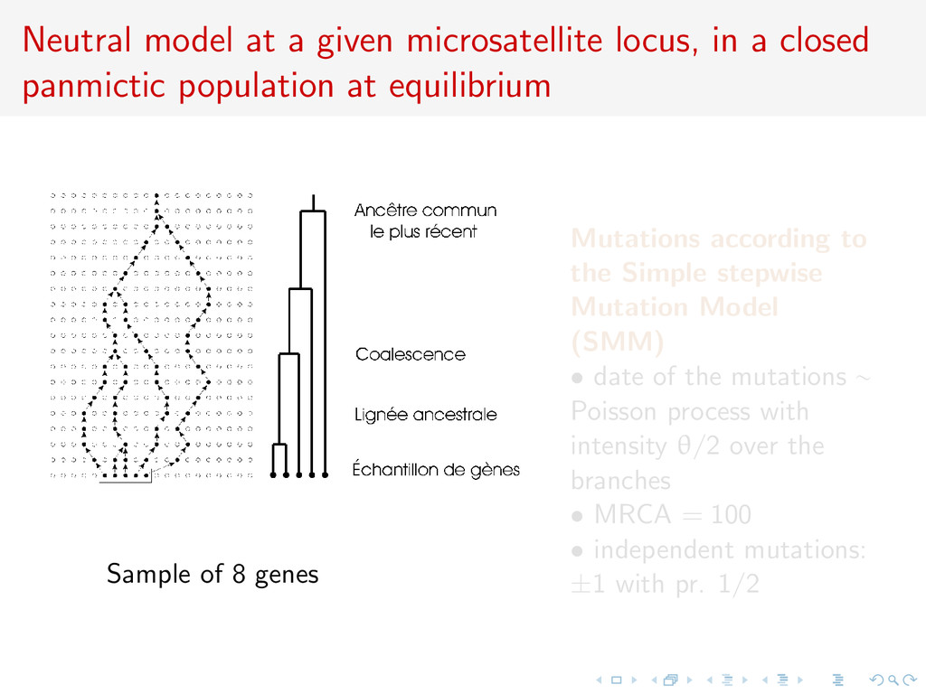
panmictic population at equilibrium Sample of 8 genes Mutations according to the Simple stepwise Mutation Model (SMM) • date of the mutations ∼ Poisson process with intensity θ/2 over the branches • MRCA = 100 • independent mutations: ±1 with pr. 1/2
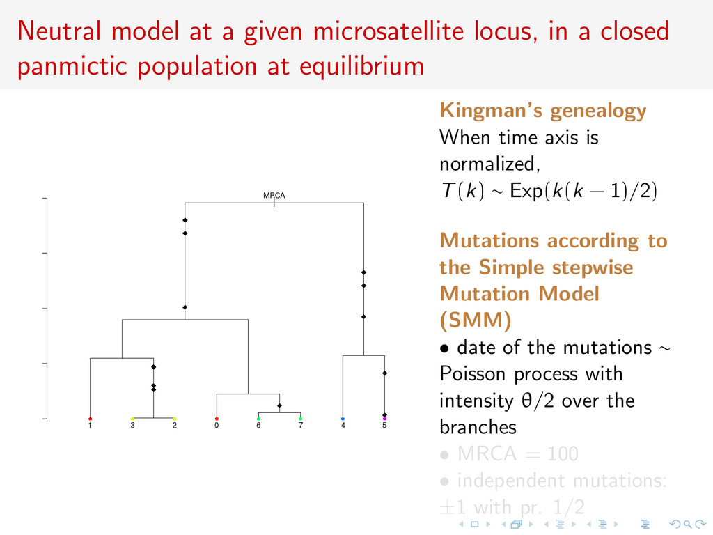
panmictic population at equilibrium Kingman’s genealogy When time axis is normalized, T(k) ∼ Exp(k(k − 1)/2) Mutations according to the Simple stepwise Mutation Model (SMM) • date of the mutations ∼ Poisson process with intensity θ/2 over the branches • MRCA = 100 • independent mutations: ±1 with pr. 1/2
panmictic population at equilibrium Kingman’s genealogy When time axis is normalized, T(k) ∼ Exp(k(k − 1)/2) Mutations according to the Simple stepwise Mutation Model (SMM) • date of the mutations ∼ Poisson process with intensity θ/2 over the branches • MRCA = 100 • independent mutations: ±1 with pr. 1/2
panmictic population at equilibrium Observations: leafs of the tree ^ θ = ? Kingman’s genealogy When time axis is normalized, T(k) ∼ Exp(k(k − 1)/2) Mutations according to the Simple stepwise Mutation Model (SMM) • date of the mutations ∼ Poisson process with intensity θ/2 over the branches • MRCA = 100 • independent mutations: ±1 with pr. 1/2
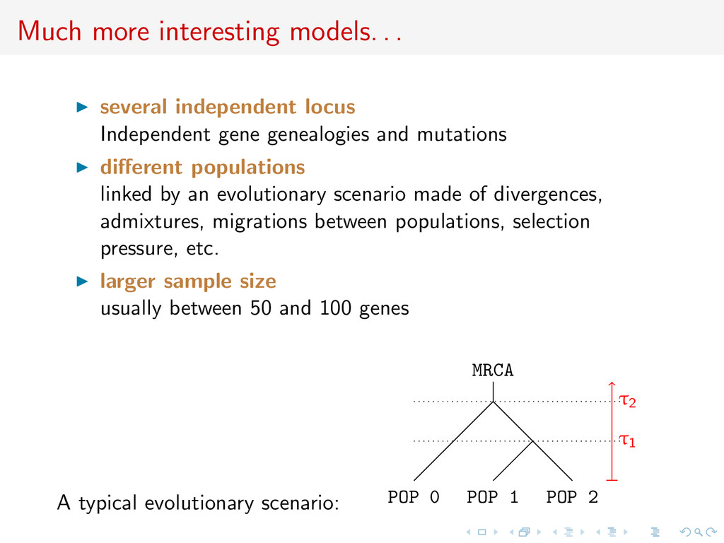
gene genealogies and mutations different populations linked by an evolutionary scenario made of divergences, admixtures, migrations between populations, selection pressure, etc. larger sample size usually between 50 and 100 genes A typical evolutionary scenario: MRCA POP 0 POP 1 POP 2 τ1 τ2
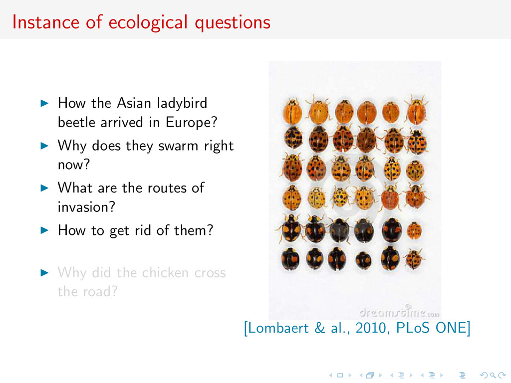
in Europe? Why does they swarm right now? What are the routes of invasion? How to get rid of them? Why did the chicken cross the road? [Lombaert & al., 2010, PLoS ONE]
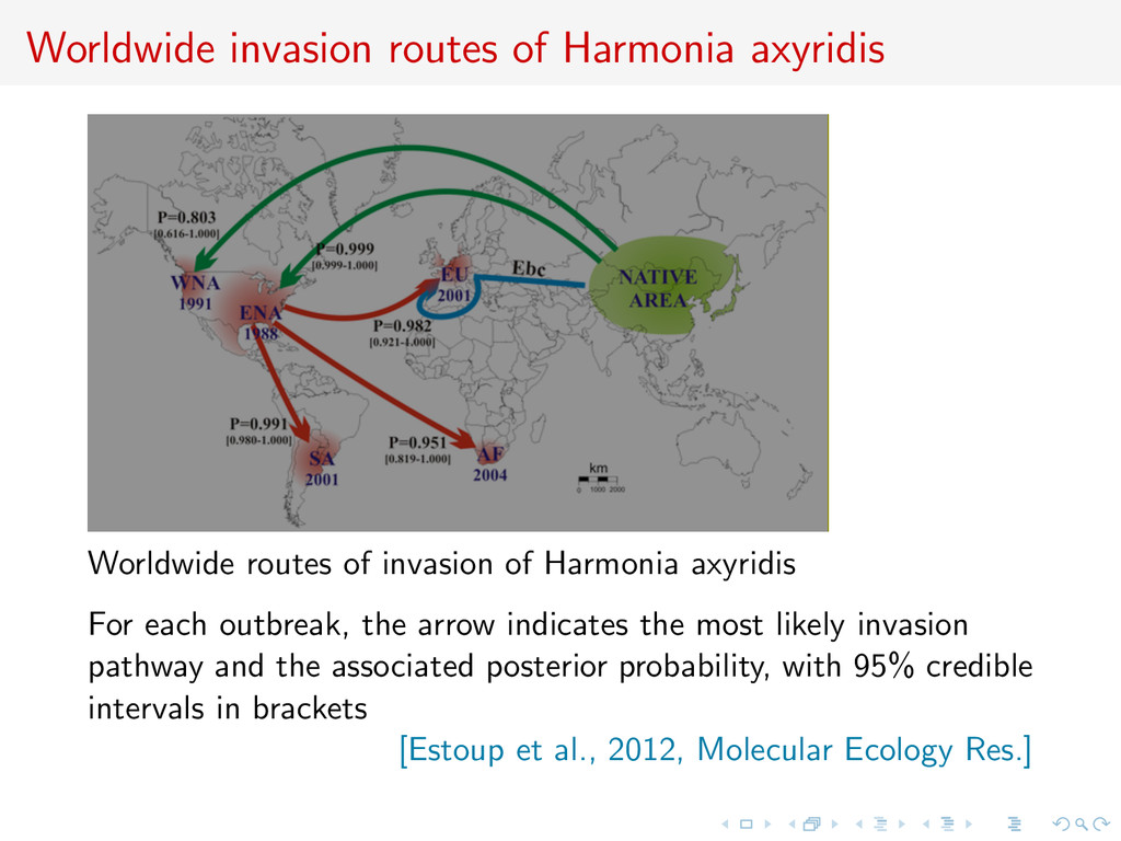
of Harmonia axyridis For each outbreak, the arrow indicates the most likely invasion pathway and the associated posterior probability, with 95% credible intervals in brackets [Estoup et al., 2012, Molecular Ecology Res.]
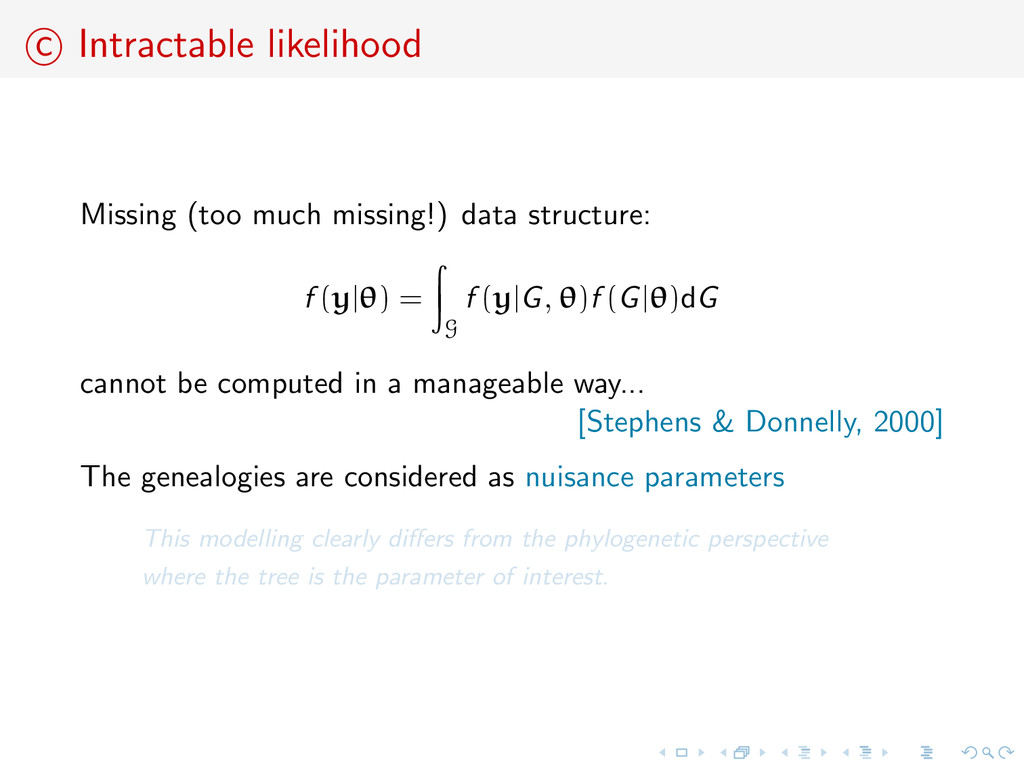
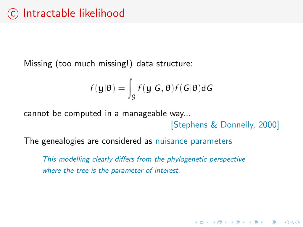
(y|θ) = G f (y|G, θ)f (G|θ)dG cannot be computed in a manageable way... [Stephens & Donnelly, 2000] The genealogies are considered as nuisance parameters This modelling clearly differs from the phylogenetic perspective where the tree is the parameter of interest.
(y|θ) = G f (y|G, θ)f (G|θ)dG cannot be computed in a manageable way... [Stephens & Donnelly, 2000] The genealogies are considered as nuisance parameters This modelling clearly differs from the phylogenetic perspective where the tree is the parameter of interest.
a Bayesian answer? ideally so (not meaningfull: requires ∞-ly powerful computer approximation error unknown (w/o costly simulation) true B for wrong model (formal and artificial) true B for noisy model (much more convincing) true B for estimated likelihood (back to econometrics?) illuminating the tension between information and precision
f (x|θ) not in closed form, likelihood-free rejection technique: Foundation For an observation y ∼ f (y|θ), under the prior π(θ), if one keeps jointly simulating θ ∼ π(θ) , z ∼ f (z|θ ) , until the auxiliary variable z is equal to the observed value, z = y, then the selected θ ∼ π(θ|y) [Rubin, 1984; Diggle & Gratton, 1984; Tavar´ e et al., 1997]
f (x|θ) not in closed form, likelihood-free rejection technique: Foundation For an observation y ∼ f (y|θ), under the prior π(θ), if one keeps jointly simulating θ ∼ π(θ) , z ∼ f (z|θ ) , until the auxiliary variable z is equal to the observed value, z = y, then the selected θ ∼ π(θ|y) [Rubin, 1984; Diggle & Gratton, 1984; Tavar´ e et al., 1997]
f (x|θ) not in closed form, likelihood-free rejection technique: Foundation For an observation y ∼ f (y|θ), under the prior π(θ), if one keeps jointly simulating θ ∼ π(θ) , z ∼ f (z|θ ) , until the auxiliary variable z is equal to the observed value, z = y, then the selected θ ∼ π(θ|y) [Rubin, 1984; Diggle & Gratton, 1984; Tavar´ e et al., 1997]
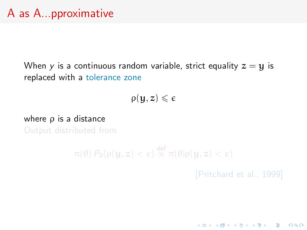
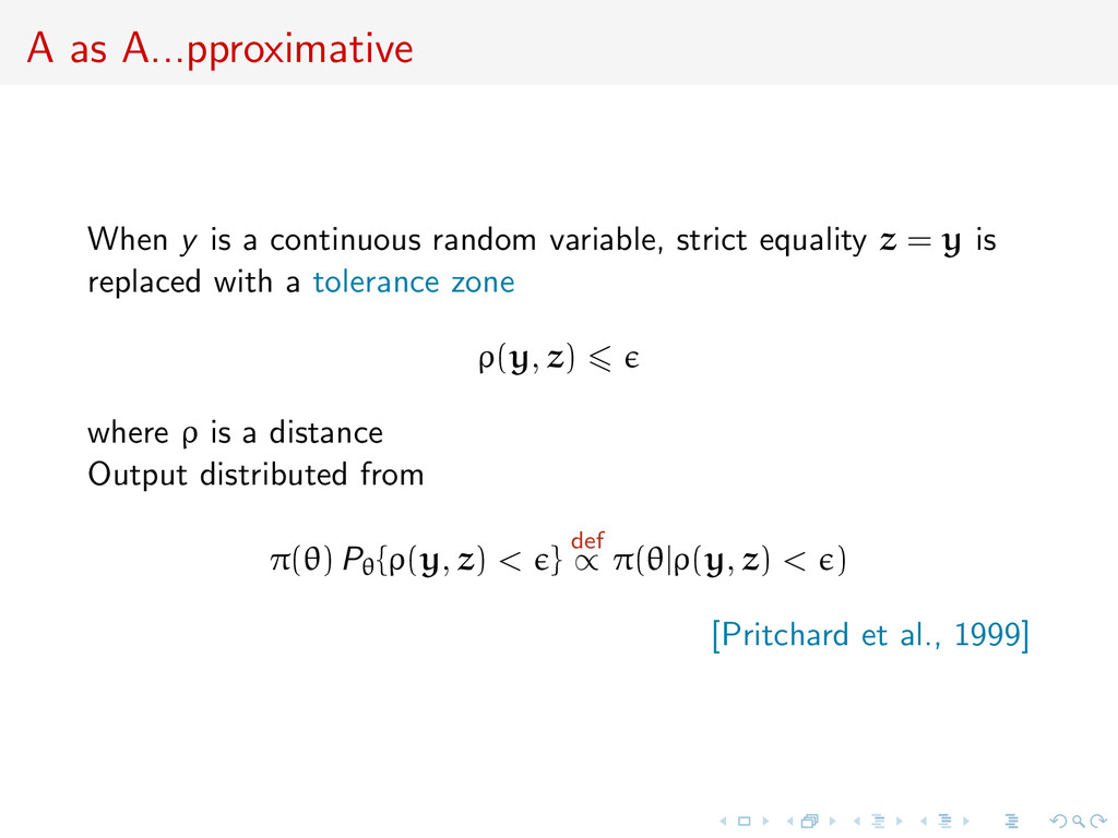
strict equality z = y is replaced with a tolerance zone ρ(y, z) where ρ is a distance Output distributed from π(θ) Pθ{ρ(y, z) < } def ∝ π(θ|ρ(y, z) < ) [Pritchard et al., 1999]
strict equality z = y is replaced with a tolerance zone ρ(y, z) where ρ is a distance Output distributed from π(θ) Pθ{ρ(y, z) < } def ∝ π(θ|ρ(y, z) < ) [Pritchard et al., 1999]
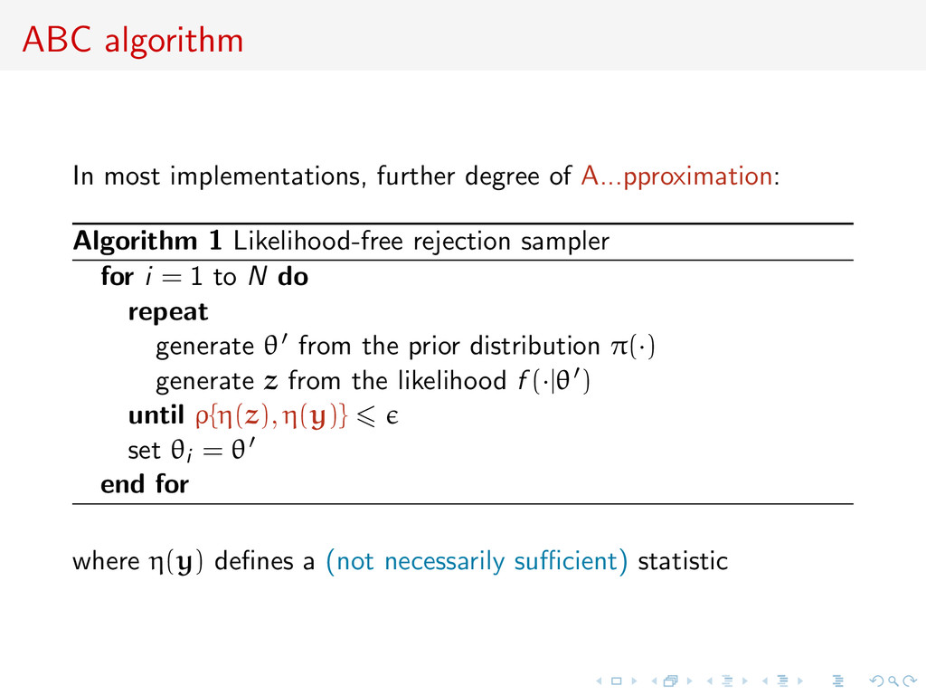
1 Likelihood-free rejection sampler for i = 1 to N do repeat generate θ from the prior distribution π(·) generate z from the likelihood f (·|θ ) until ρ{η(z), η(y)} set θi = θ end for where η(y) defines a (not necessarily sufficient) statistic
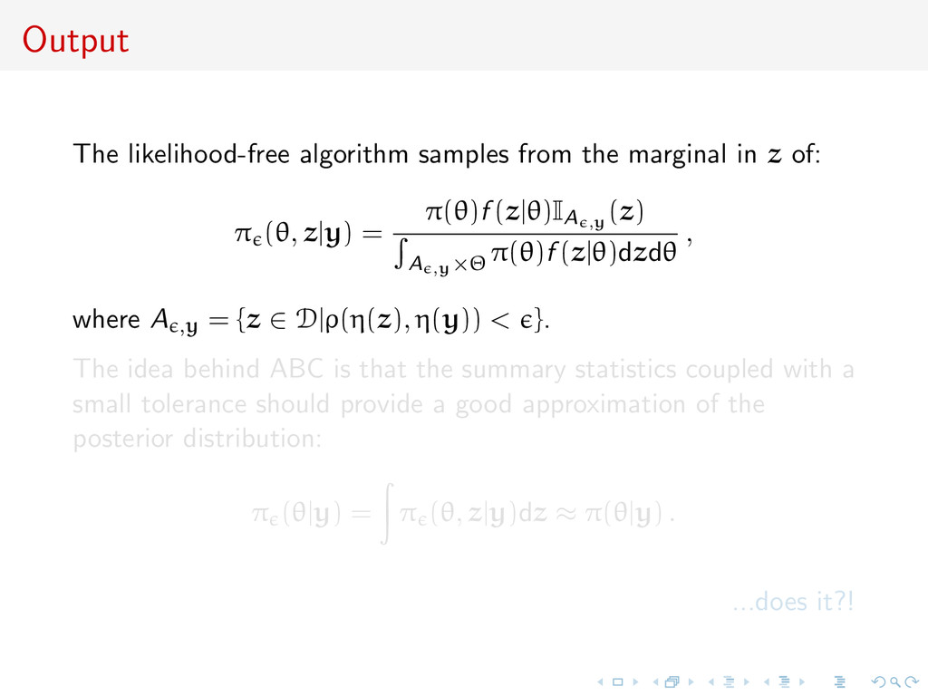
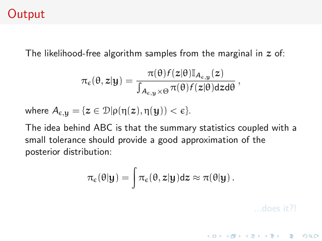
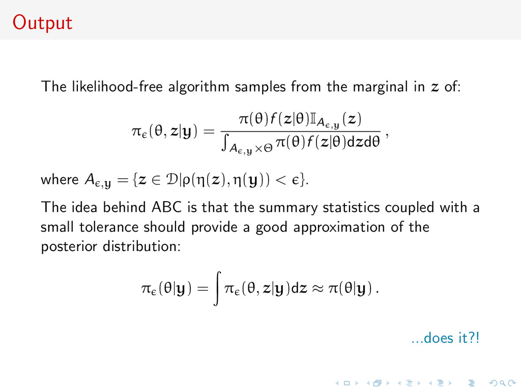
of: π (θ, z|y) = π(θ)f (z|θ)IA ,y (z) A ,y×Θ π(θ)f (z|θ)dzdθ , where A ,y = {z ∈ D|ρ(η(z), η(y)) < }. The idea behind ABC is that the summary statistics coupled with a small tolerance should provide a good approximation of the posterior distribution: π (θ|y) = π (θ, z|y)dz ≈ π(θ|y) . ...does it?!
of: π (θ, z|y) = π(θ)f (z|θ)IA ,y (z) A ,y×Θ π(θ)f (z|θ)dzdθ , where A ,y = {z ∈ D|ρ(η(z), η(y)) < }. The idea behind ABC is that the summary statistics coupled with a small tolerance should provide a good approximation of the posterior distribution: π (θ|y) = π (θ, z|y)dz ≈ π(θ|y) . ...does it?!
of: π (θ, z|y) = π(θ)f (z|θ)IA ,y (z) A ,y×Θ π(θ)f (z|θ)dzdθ , where A ,y = {z ∈ D|ρ(η(z), η(y)) < }. The idea behind ABC is that the summary statistics coupled with a small tolerance should provide a good approximation of the posterior distribution: π (θ|y) = π (θ, z|y)dz ≈ π(θ|y) . ...does it?!
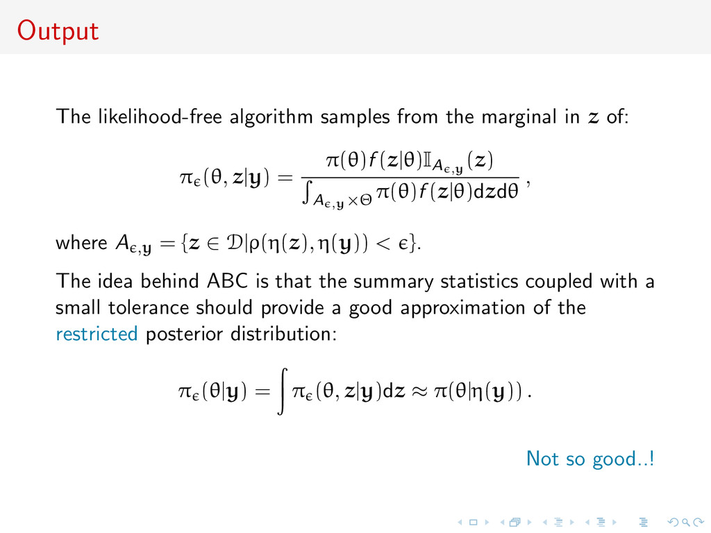
of: π (θ, z|y) = π(θ)f (z|θ)IA ,y (z) A ,y×Θ π(θ)f (z|θ)dzdθ , where A ,y = {z ∈ D|ρ(η(z), η(y)) < }. The idea behind ABC is that the summary statistics coupled with a small tolerance should provide a good approximation of the restricted posterior distribution: π (θ|y) = π (θ, z|y)dz ≈ π(θ|η(y)) . Not so good..!
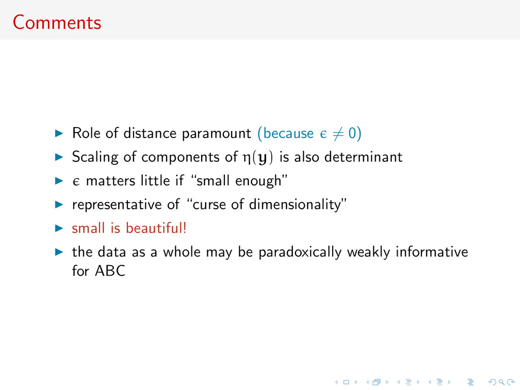
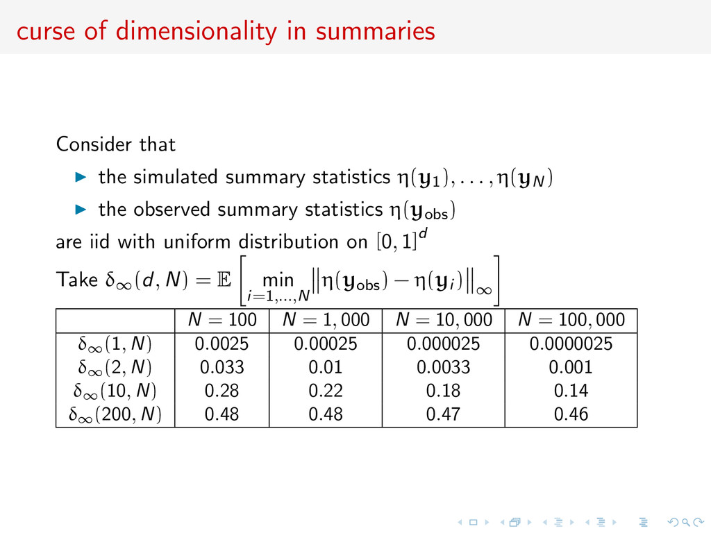
components of η(y) is also determinant matters little if “small enough” representative of “curse of dimensionality” small is beautiful! the data as a whole may be paradoxically weakly informative for ABC
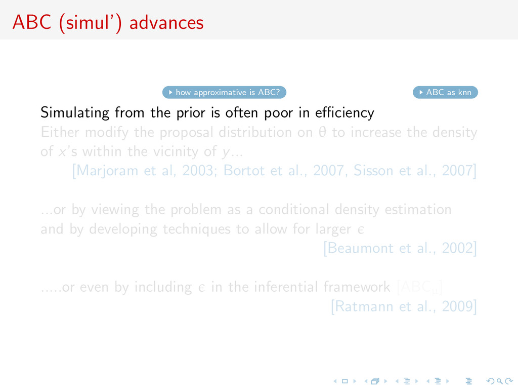
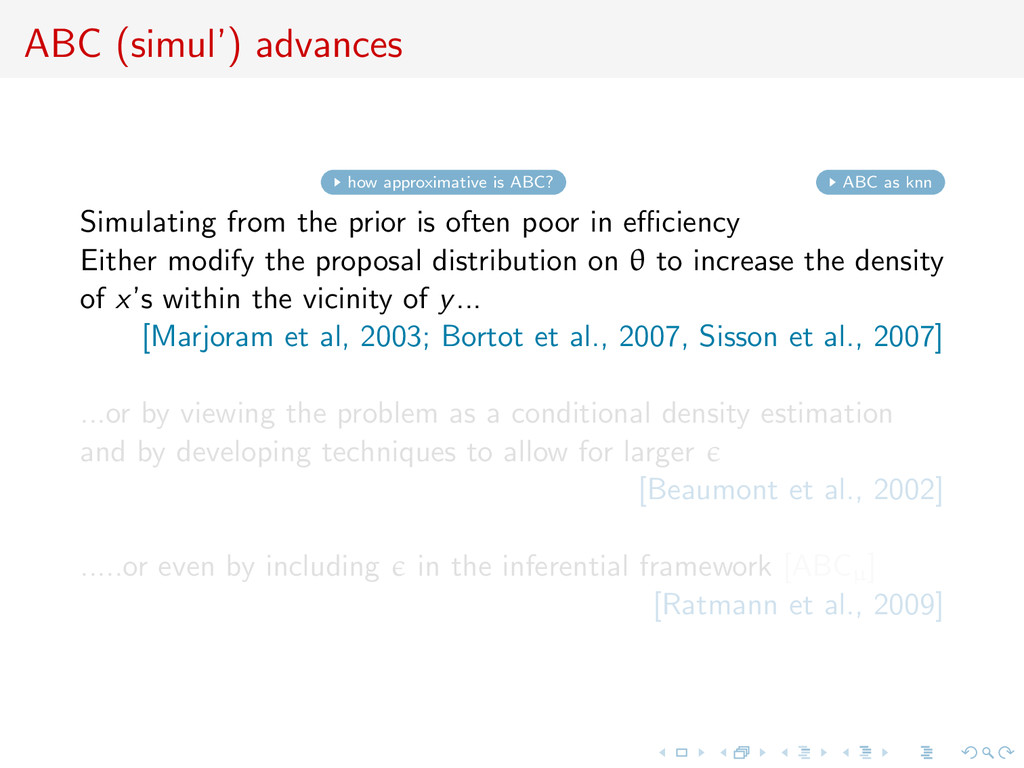
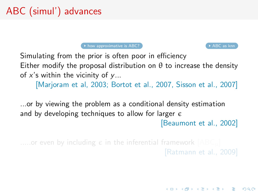
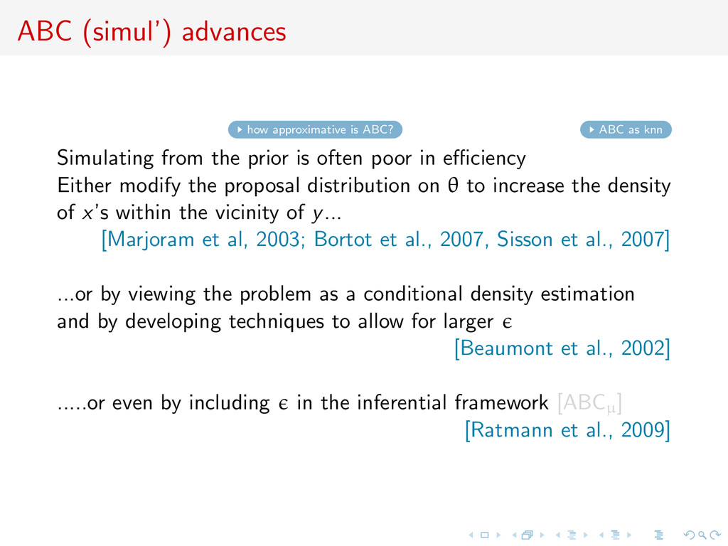
Simulating from the prior is often poor in efficiency Either modify the proposal distribution on θ to increase the density of x’s within the vicinity of y... [Marjoram et al, 2003; Bortot et al., 2007, Sisson et al., 2007] ...or by viewing the problem as a conditional density estimation and by developing techniques to allow for larger [Beaumont et al., 2002] .....or even by including in the inferential framework [ABCµ] [Ratmann et al., 2009]
Simulating from the prior is often poor in efficiency Either modify the proposal distribution on θ to increase the density of x’s within the vicinity of y... [Marjoram et al, 2003; Bortot et al., 2007, Sisson et al., 2007] ...or by viewing the problem as a conditional density estimation and by developing techniques to allow for larger [Beaumont et al., 2002] .....or even by including in the inferential framework [ABCµ] [Ratmann et al., 2009]
Simulating from the prior is often poor in efficiency Either modify the proposal distribution on θ to increase the density of x’s within the vicinity of y... [Marjoram et al, 2003; Bortot et al., 2007, Sisson et al., 2007] ...or by viewing the problem as a conditional density estimation and by developing techniques to allow for larger [Beaumont et al., 2002] .....or even by including in the inferential framework [ABCµ] [Ratmann et al., 2009]
Simulating from the prior is often poor in efficiency Either modify the proposal distribution on θ to increase the density of x’s within the vicinity of y... [Marjoram et al, 2003; Bortot et al., 2007, Sisson et al., 2007] ...or by viewing the problem as a conditional density estimation and by developing techniques to allow for larger [Beaumont et al., 2002] .....or even by including in the inferential framework [ABCµ] [Ratmann et al., 2009]
Practice of ABC: determine tolerance as a quantile on observed distances, say 10% or 1% quantile, = N = qα(d1, . . . , dN) Interpretation of ε as nonparametric bandwidth only approximation of the actual practice [Blum & Fran¸ cois, 2010] ABC is a k-nearest neighbour (knn) method with kN = N N [Loftsgaarden & Quesenberry, 1965]
Practice of ABC: determine tolerance as a quantile on observed distances, say 10% or 1% quantile, = N = qα(d1, . . . , dN) Interpretation of ε as nonparametric bandwidth only approximation of the actual practice [Blum & Fran¸ cois, 2010] ABC is a k-nearest neighbour (knn) method with kN = N N [Loftsgaarden & Quesenberry, 1965]
Practice of ABC: determine tolerance as a quantile on observed distances, say 10% or 1% quantile, = N = qα(d1, . . . , dN) Interpretation of ε as nonparametric bandwidth only approximation of the actual practice [Blum & Fran¸ cois, 2010] ABC is a k-nearest neighbour (knn) method with kN = N N [Loftsgaarden & Quesenberry, 1965]
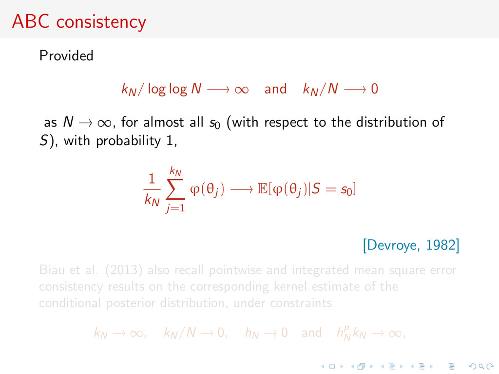
kN/N −→ 0 as N → ∞, for almost all s0 (with respect to the distribution of S), with probability 1, 1 kN kN j=1 ϕ(θj ) −→ E[ϕ(θj )|S = s0] [Devroye, 1982] Biau et al. (2013) also recall pointwise and integrated mean square error consistency results on the corresponding kernel estimate of the conditional posterior distribution, under constraints kN → ∞, kN /N → 0, hN → 0 and hp N kN → ∞,
kN/N −→ 0 as N → ∞, for almost all s0 (with respect to the distribution of S), with probability 1, 1 kN kN j=1 ϕ(θj ) −→ E[ϕ(θj )|S = s0] [Devroye, 1982] Biau et al. (2013) also recall pointwise and integrated mean square error consistency results on the corresponding kernel estimate of the conditional posterior distribution, under constraints kN → ∞, kN /N → 0, hN → 0 and hp N kN → ∞,
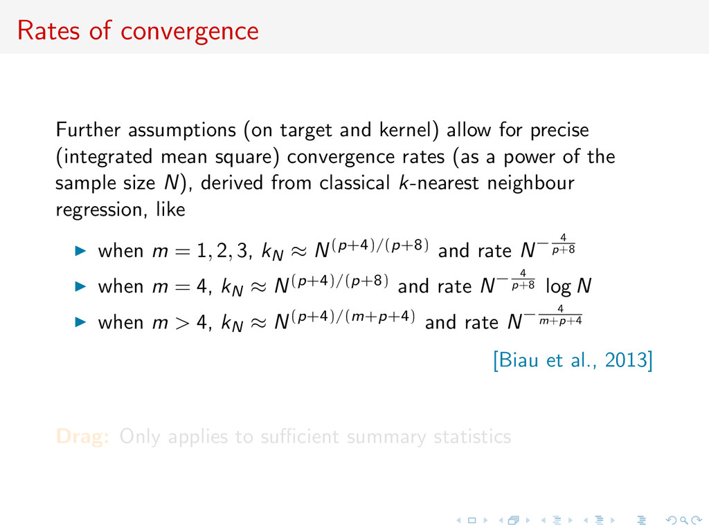
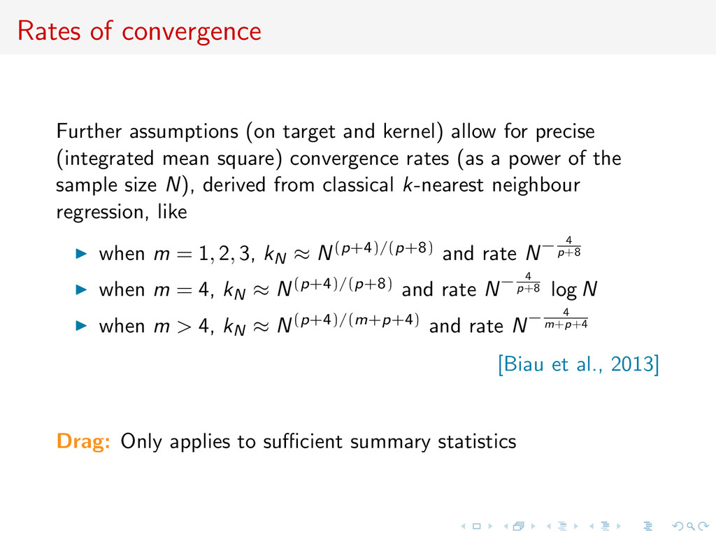
for precise (integrated mean square) convergence rates (as a power of the sample size N), derived from classical k-nearest neighbour regression, like when m = 1, 2, 3, kN ≈ N(p+4)/(p+8) and rate N− 4 p+8 when m = 4, kN ≈ N(p+4)/(p+8) and rate N− 4 p+8 log N when m > 4, kN ≈ N(p+4)/(m+p+4) and rate N− 4 m+p+4 [Biau et al., 2013] Drag: Only applies to sufficient summary statistics
for precise (integrated mean square) convergence rates (as a power of the sample size N), derived from classical k-nearest neighbour regression, like when m = 1, 2, 3, kN ≈ N(p+4)/(p+8) and rate N− 4 p+8 when m = 4, kN ≈ N(p+4)/(p+8) and rate N− 4 p+8 log N when m > 4, kN ≈ N(p+4)/(m+p+4) and rate N− 4 m+p+4 [Biau et al., 2013] Drag: Only applies to sufficient summary statistics
inference machine Error inc. Exact BC and approximate targets summary statistic ABC for model choice Model choice consistency Conclusion and perspectives
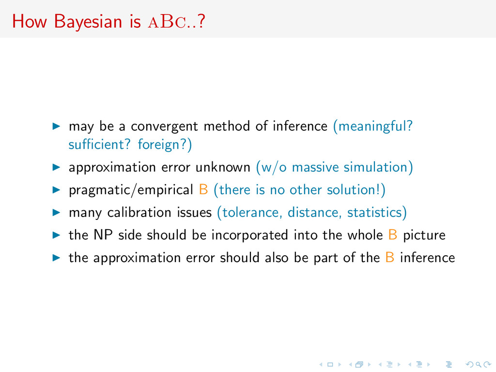
inference (meaningful? sufficient? foreign?) approximation error unknown (w/o massive simulation) pragmatic/empirical B (there is no other solution!) many calibration issues (tolerance, distance, statistics) the NP side should be incorporated into the whole B picture the approximation error should also be part of the B inference
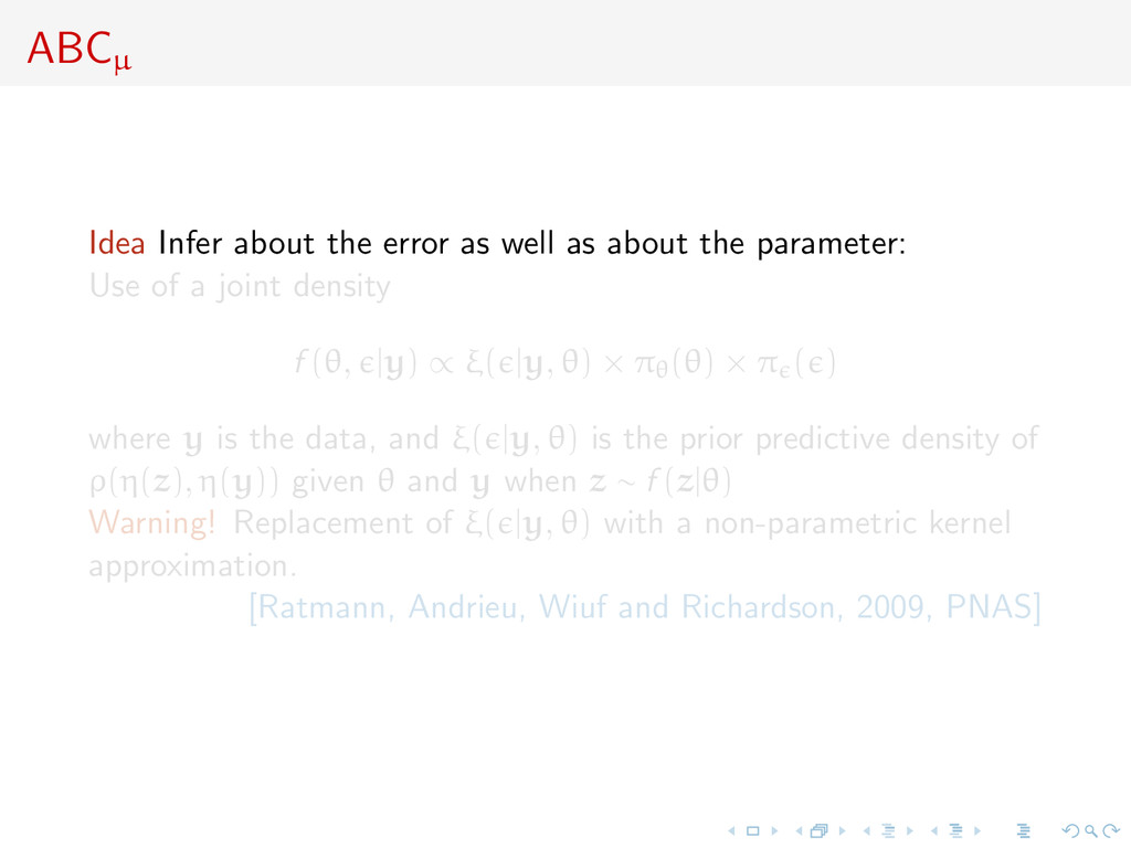
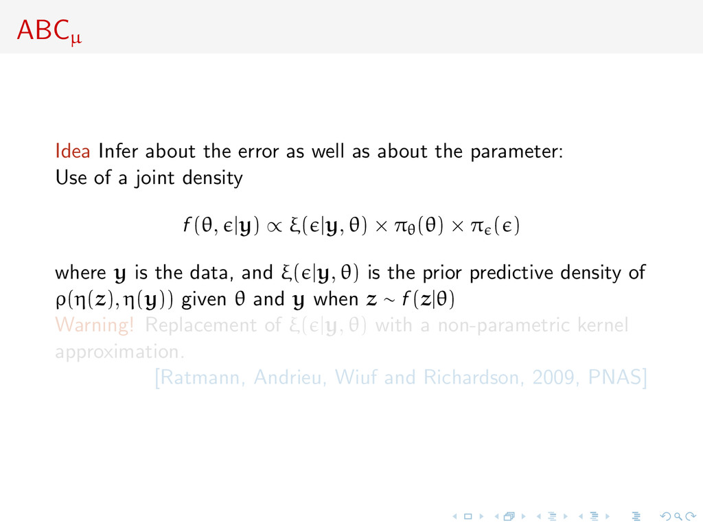
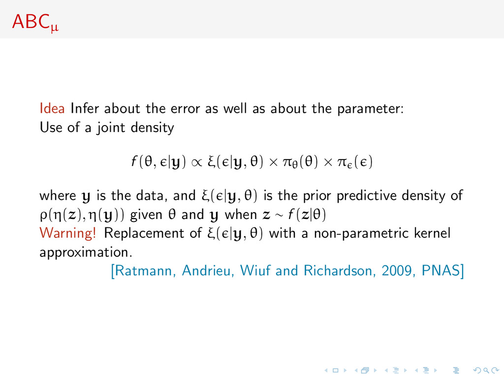
the parameter: Use of a joint density f (θ, |y) ∝ ξ( |y, θ) × πθ(θ) × π ( ) where y is the data, and ξ( |y, θ) is the prior predictive density of ρ(η(z), η(y)) given θ and y when z ∼ f (z|θ) Warning! Replacement of ξ( |y, θ) with a non-parametric kernel approximation. [Ratmann, Andrieu, Wiuf and Richardson, 2009, PNAS]
the parameter: Use of a joint density f (θ, |y) ∝ ξ( |y, θ) × πθ(θ) × π ( ) where y is the data, and ξ( |y, θ) is the prior predictive density of ρ(η(z), η(y)) given θ and y when z ∼ f (z|θ) Warning! Replacement of ξ( |y, θ) with a non-parametric kernel approximation. [Ratmann, Andrieu, Wiuf and Richardson, 2009, PNAS]
the parameter: Use of a joint density f (θ, |y) ∝ ξ( |y, θ) × πθ(θ) × π ( ) where y is the data, and ξ( |y, θ) is the prior predictive density of ρ(η(z), η(y)) given θ and y when z ∼ f (z|θ) Warning! Replacement of ξ( |y, θ) with a non-parametric kernel approximation. [Ratmann, Andrieu, Wiuf and Richardson, 2009, PNAS]
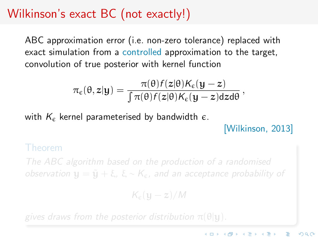
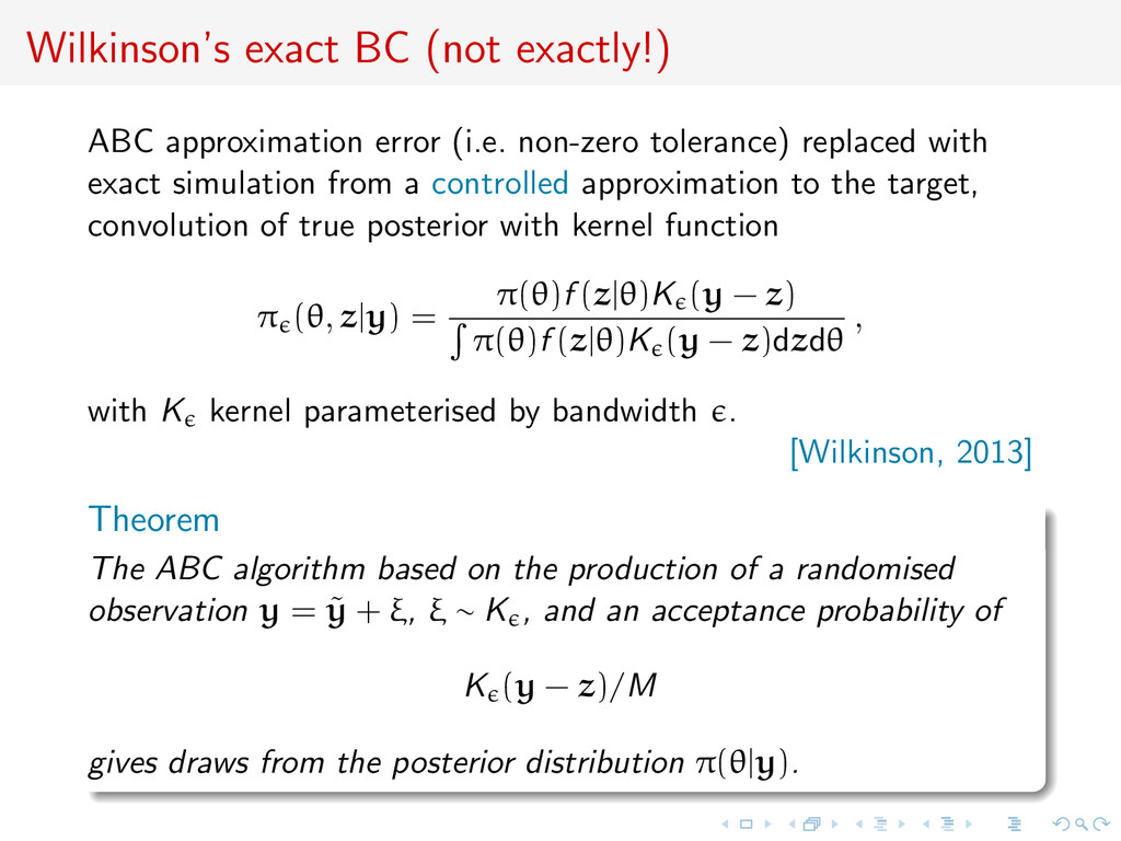
tolerance) replaced with exact simulation from a controlled approximation to the target, convolution of true posterior with kernel function π (θ, z|y) = π(θ)f (z|θ)K (y − z) π(θ)f (z|θ)K (y − z)dzdθ , with K kernel parameterised by bandwidth . [Wilkinson, 2013] Theorem The ABC algorithm based on the production of a randomised observation y = ˜ y + ξ, ξ ∼ K , and an acceptance probability of K (y − z)/M gives draws from the posterior distribution π(θ|y).
tolerance) replaced with exact simulation from a controlled approximation to the target, convolution of true posterior with kernel function π (θ, z|y) = π(θ)f (z|θ)K (y − z) π(θ)f (z|θ)K (y − z)dzdθ , with K kernel parameterised by bandwidth . [Wilkinson, 2013] Theorem The ABC algorithm based on the production of a randomised observation y = ˜ y + ξ, ξ ∼ K , and an acceptance probability of K (y − z)/M gives draws from the posterior distribution π(θ|y).
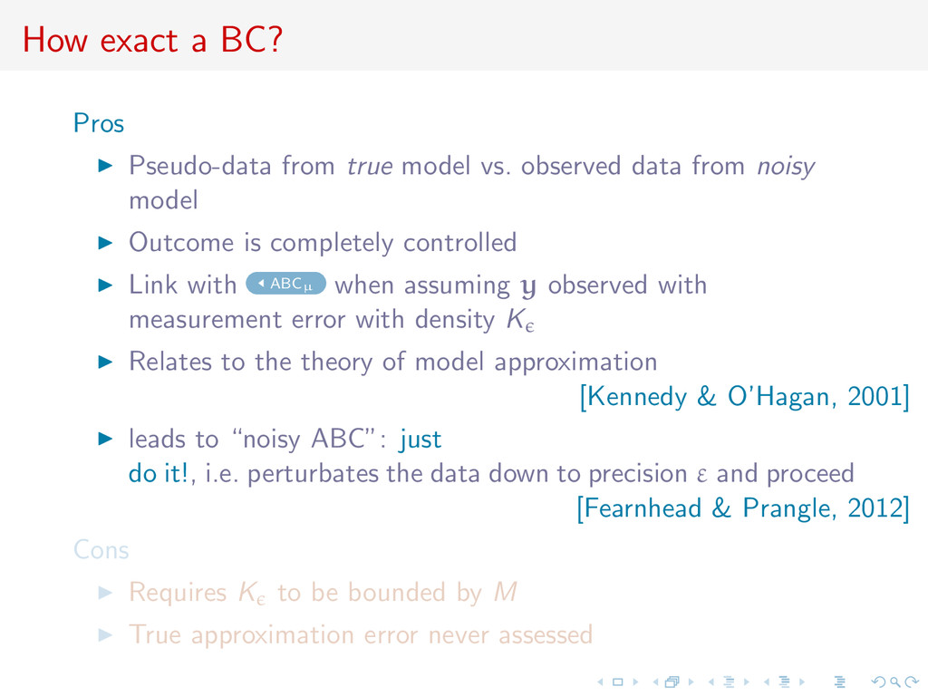
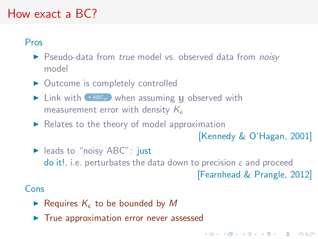
observed data from noisy model Outcome is completely controlled Link with ABCµ when assuming y observed with measurement error with density K Relates to the theory of model approximation [Kennedy & O’Hagan, 2001] leads to “noisy ABC”: just do it!, i.e. perturbates the data down to precision ε and proceed [Fearnhead & Prangle, 2012] Cons Requires K to be bounded by M True approximation error never assessed
observed data from noisy model Outcome is completely controlled Link with ABCµ when assuming y observed with measurement error with density K Relates to the theory of model approximation [Kennedy & O’Hagan, 2001] leads to “noisy ABC”: just do it!, i.e. perturbates the data down to precision ε and proceed [Fearnhead & Prangle, 2012] Cons Requires K to be bounded by M True approximation error never assessed
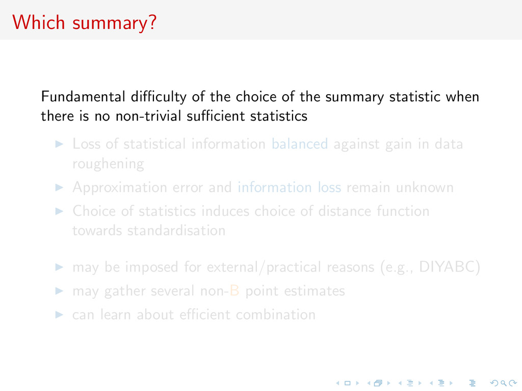
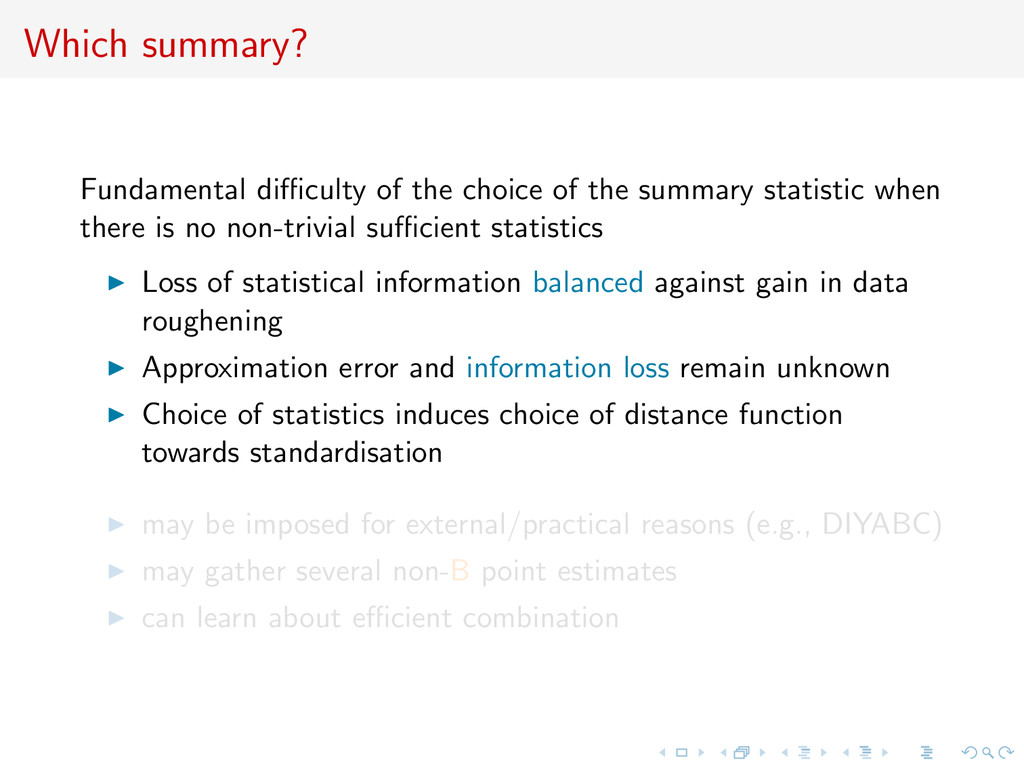
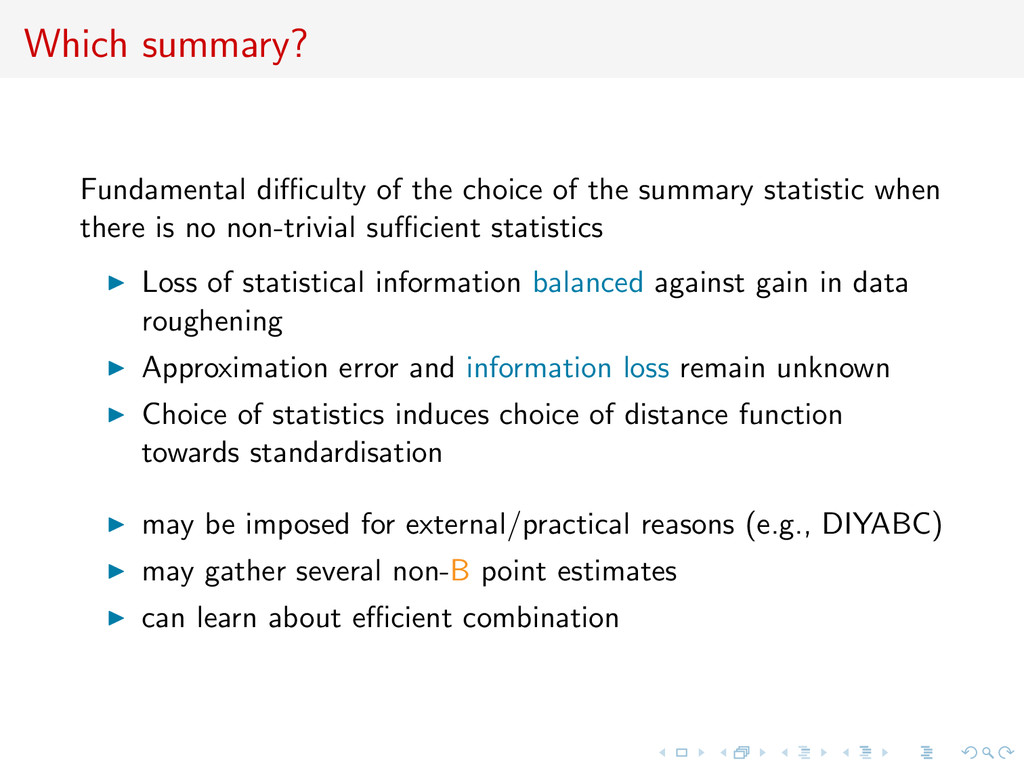
statistic when there is no non-trivial sufficient statistics Loss of statistical information balanced against gain in data roughening Approximation error and information loss remain unknown Choice of statistics induces choice of distance function towards standardisation may be imposed for external/practical reasons (e.g., DIYABC) may gather several non-B point estimates can learn about efficient combination
statistic when there is no non-trivial sufficient statistics Loss of statistical information balanced against gain in data roughening Approximation error and information loss remain unknown Choice of statistics induces choice of distance function towards standardisation may be imposed for external/practical reasons (e.g., DIYABC) may gather several non-B point estimates can learn about efficient combination
statistic when there is no non-trivial sufficient statistics Loss of statistical information balanced against gain in data roughening Approximation error and information loss remain unknown Choice of statistics induces choice of distance function towards standardisation may be imposed for external/practical reasons (e.g., DIYABC) may gather several non-B point estimates can learn about efficient combination
selection of the summary statistic in close proximity to Wilkinson’s proposal ABC considered as inferential method and calibrated as such randomised (or ‘noisy’) version of the summary statistics ˜ η(y) = η(y) + τ derivation of a well-calibrated version of ABC, i.e. an algorithm that gives proper predictions for the distribution associated with this randomised summary statistic [weak property]
the parameter of interest as summary statistics η(y)! [requires iterative process] use of the standard quadratic loss function (θ − θ0)TA(θ − θ0) recent extension to model choice, optimality of Bayes factor B12(y) [F&P, ISBA 2012, Kyoto]
the parameter of interest as summary statistics η(y)! [requires iterative process] use of the standard quadratic loss function (θ − θ0)TA(θ − θ0) recent extension to model choice, optimality of Bayes factor B12(y) [F&P, ISBA 2012, Kyoto]
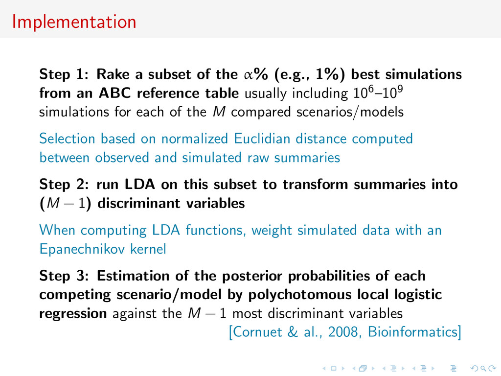
semi-automatic ABC, selection of most discriminant subvector out of a collection of summary statistics, based on Linear Discriminant Analysis (LDA) [Estoup & al., 2012, Mol. Ecol. Res.] Solution now implemented in DIYABC.2 [Cornuet & al., 2008, Bioinf.; Estoup & al., 2013]
1%) best simulations from an ABC reference table usually including 106–109 simulations for each of the M compared scenarios/models Selection based on normalized Euclidian distance computed between observed and simulated raw summaries Step 2: run LDA on this subset to transform summaries into (M − 1) discriminant variables When computing LDA functions, weight simulated data with an Epanechnikov kernel Step 3: Estimation of the posterior probabilities of each competing scenario/model by polychotomous local logistic regression against the M − 1 most discriminant variables [Cornuet & al., 2008, Bioinformatics]
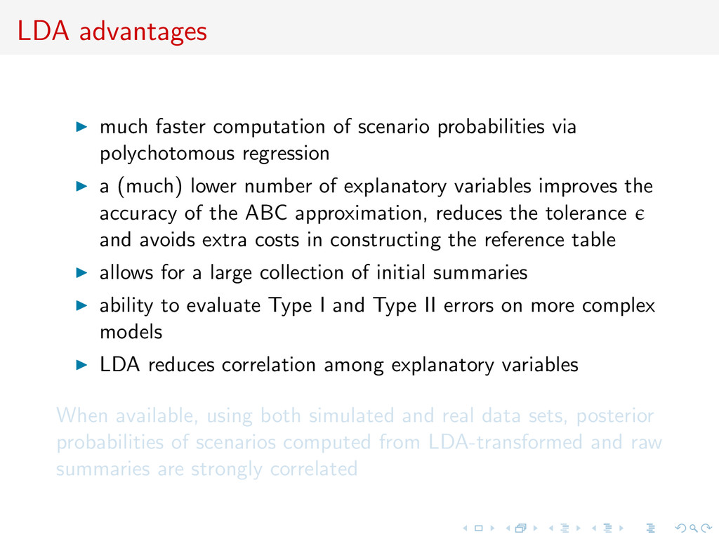
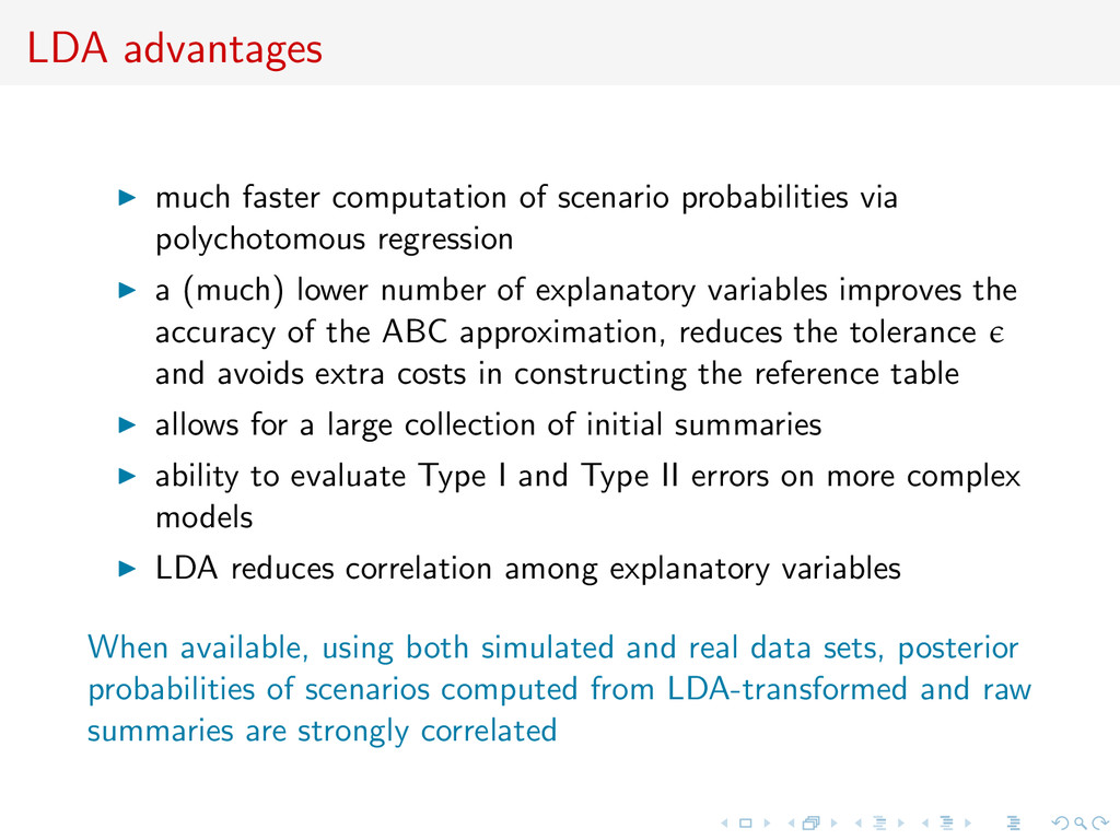
regression a (much) lower number of explanatory variables improves the accuracy of the ABC approximation, reduces the tolerance and avoids extra costs in constructing the reference table allows for a large collection of initial summaries ability to evaluate Type I and Type II errors on more complex models LDA reduces correlation among explanatory variables When available, using both simulated and real data sets, posterior probabilities of scenarios computed from LDA-transformed and raw summaries are strongly correlated
regression a (much) lower number of explanatory variables improves the accuracy of the ABC approximation, reduces the tolerance and avoids extra costs in constructing the reference table allows for a large collection of initial summaries ability to evaluate Type I and Type II errors on more complex models LDA reduces correlation among explanatory variables When available, using both simulated and real data sets, posterior probabilities of scenarios computed from LDA-transformed and raw summaries are strongly correlated
an inference machine ABC for model choice BMC Principle Gibbs random fields (counterexample) Generic ABC model choice Model choice consistency Conclusion and perspectives
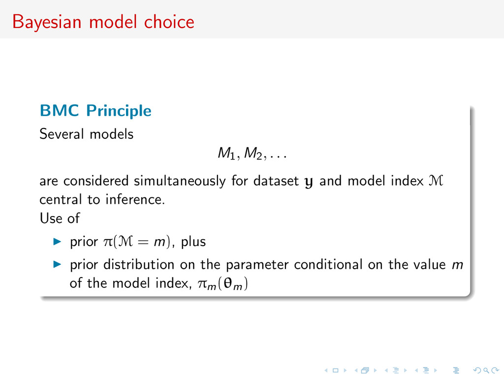
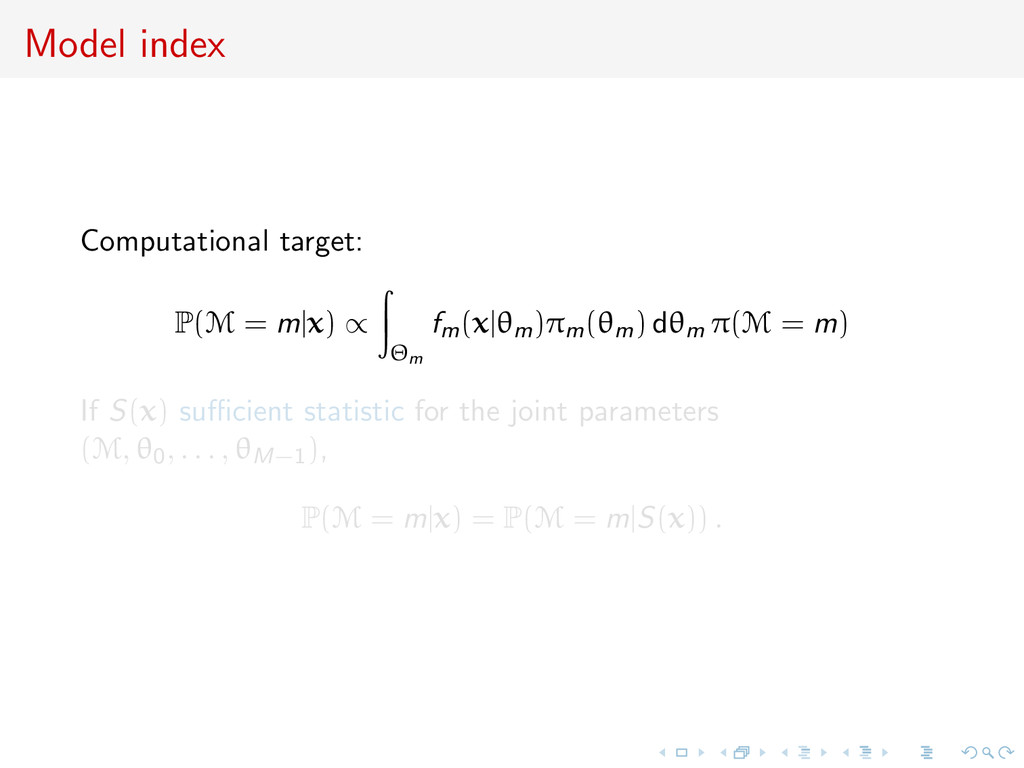
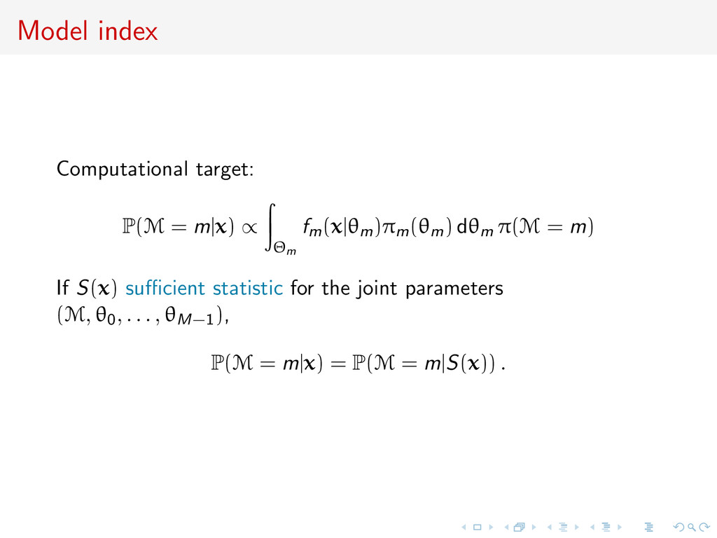
. . are considered simultaneously for dataset y and model index M central to inference. Use of prior π(M = m), plus prior distribution on the parameter conditional on the value m of the model index, πm(θm)
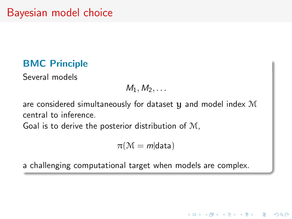
. . are considered simultaneously for dataset y and model index M central to inference. Goal is to derive the posterior distribution of M, π(M = m|data) a challenging computational target when models are complex.
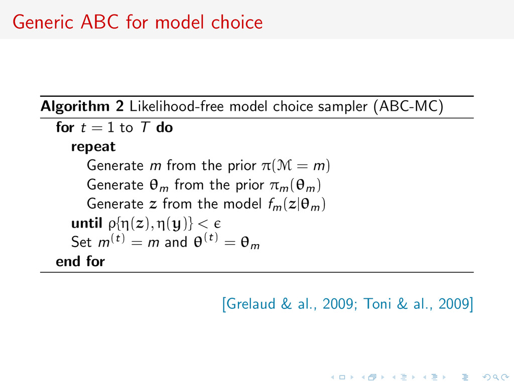
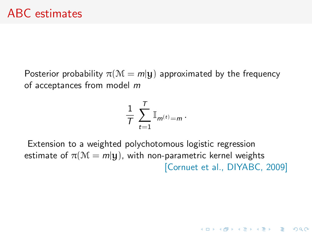
sampler (ABC-MC) for t = 1 to T do repeat Generate m from the prior π(M = m) Generate θm from the prior πm(θm) Generate z from the model fm(z|θm) until ρ{η(z), η(y)} < Set m(t) = m and θ(t) = θm end for [Grelaud & al., 2009; Toni & al., 2009]
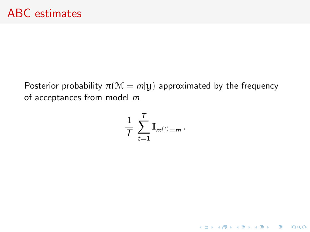
frequency of acceptances from model m 1 T T t=1 Im(t)=m . Extension to a weighted polychotomous logistic regression estimate of π(M = m|y), with non-parametric kernel weights [Cornuet et al., DIYABC, 2009]
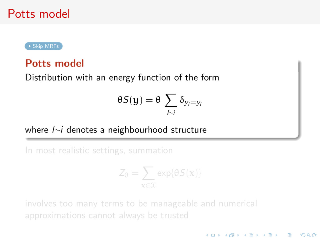
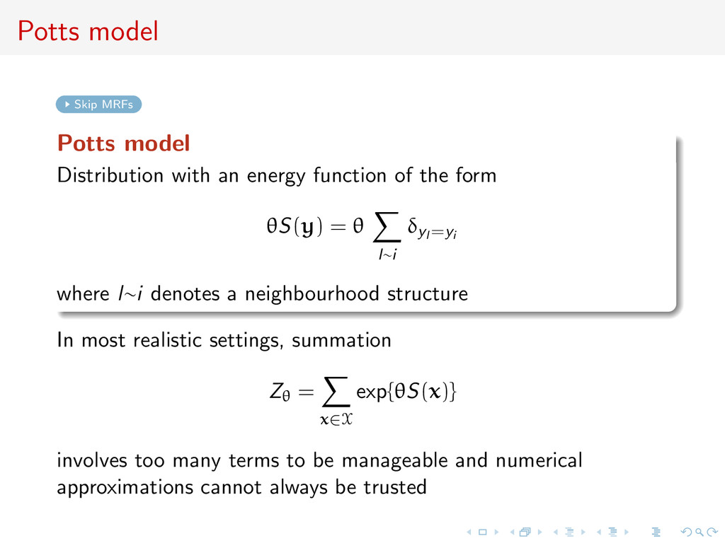
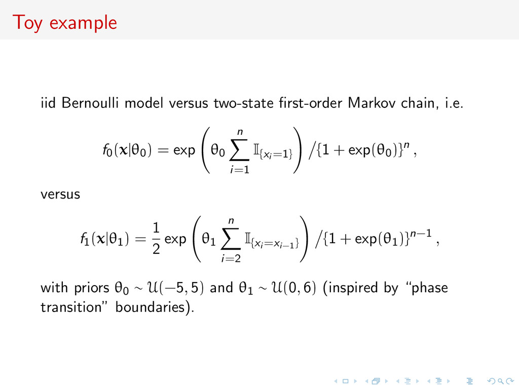
function of the form θS(y) = θ l∼i δyl =yi where l∼i denotes a neighbourhood structure In most realistic settings, summation Zθ = x∈X exp{θS(x)} involves too many terms to be manageable and numerical approximations cannot always be trusted
function of the form θS(y) = θ l∼i δyl =yi where l∼i denotes a neighbourhood structure In most realistic settings, summation Zθ = x∈X exp{θS(x)} involves too many terms to be manageable and numerical approximations cannot always be trusted
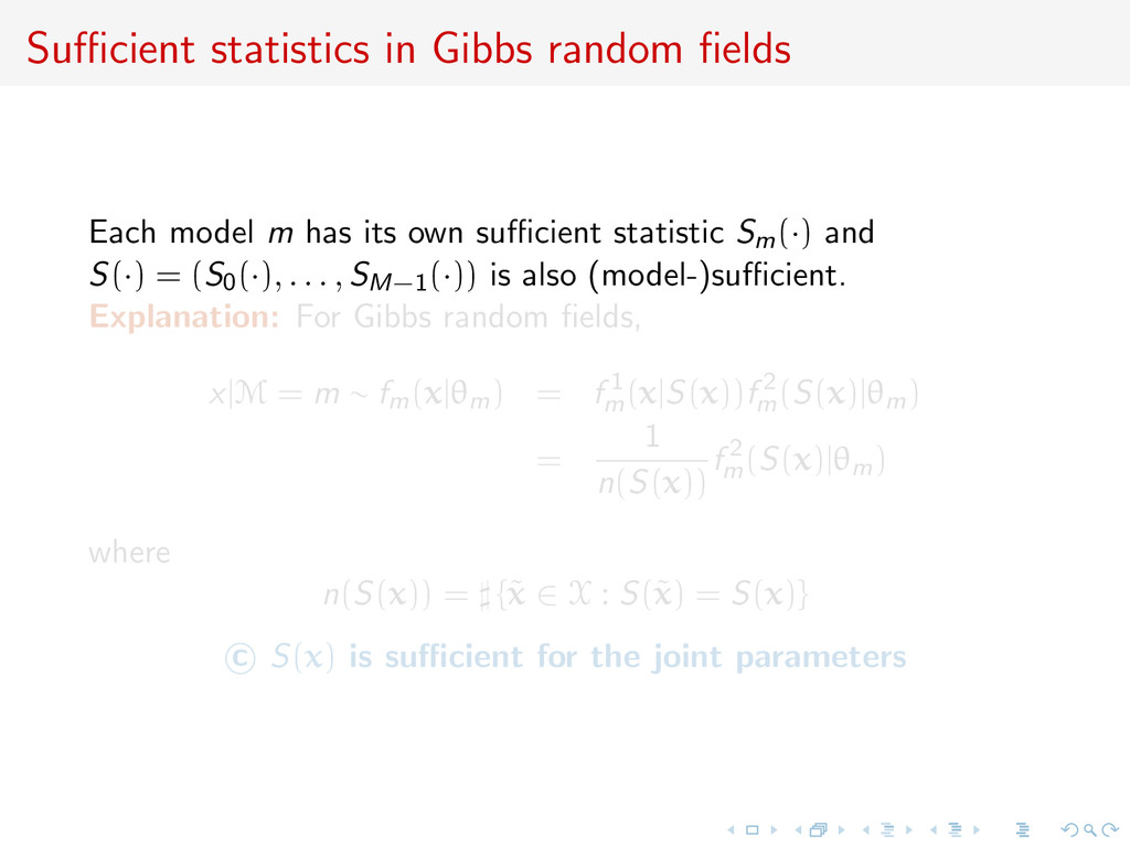
its own sufficient statistic Sm(·) and S(·) = (S0(·), . . . , SM−1(·)) is also (model-)sufficient. Explanation: For Gibbs random fields, x|M = m ∼ fm(x|θm) = f 1 m (x|S(x))f 2 m (S(x)|θm) = 1 n(S(x)) f 2 m (S(x)|θm) where n(S(x)) = {˜ x ∈ X : S(˜ x) = S(x)} c S(x) is sufficient for the joint parameters
its own sufficient statistic Sm(·) and S(·) = (S0(·), . . . , SM−1(·)) is also (model-)sufficient. Explanation: For Gibbs random fields, x|M = m ∼ fm(x|θm) = f 1 m (x|S(x))f 2 m (S(x)|θm) = 1 n(S(x)) f 2 m (S(x)|θm) where n(S(x)) = {˜ x ∈ X : S(˜ x) = S(x)} c S(x) is sufficient for the joint parameters
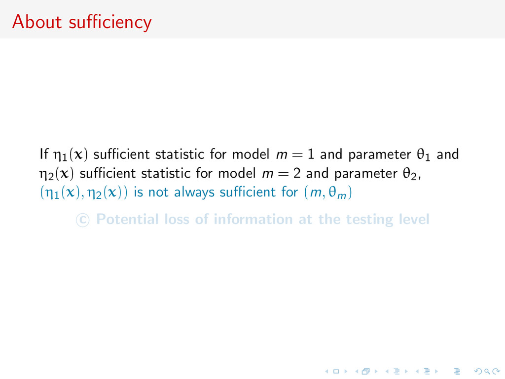
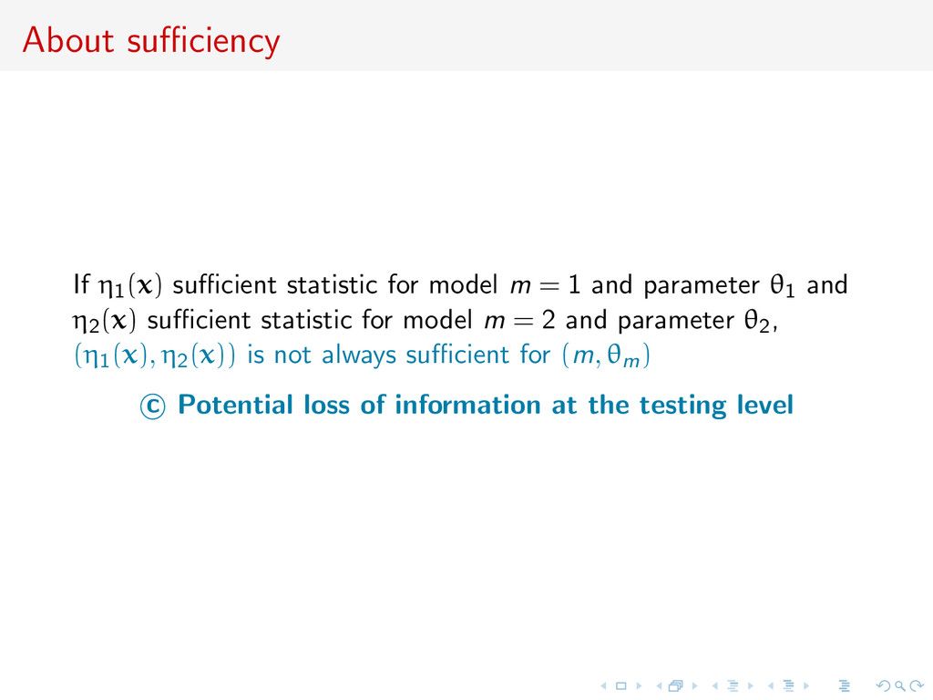
1 and parameter θ1 and η2(x) sufficient statistic for model m = 2 and parameter θ2, (η1(x), η2(x)) is not always sufficient for (m, θm) c Potential loss of information at the testing level
1 and parameter θ1 and η2(x) sufficient statistic for model m = 2 and parameter θ2, (η1(x), η2(x)) is not always sufficient for (m, θm) c Potential loss of information at the testing level
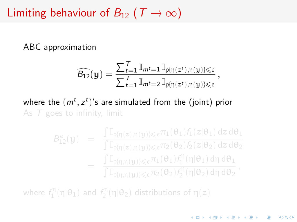
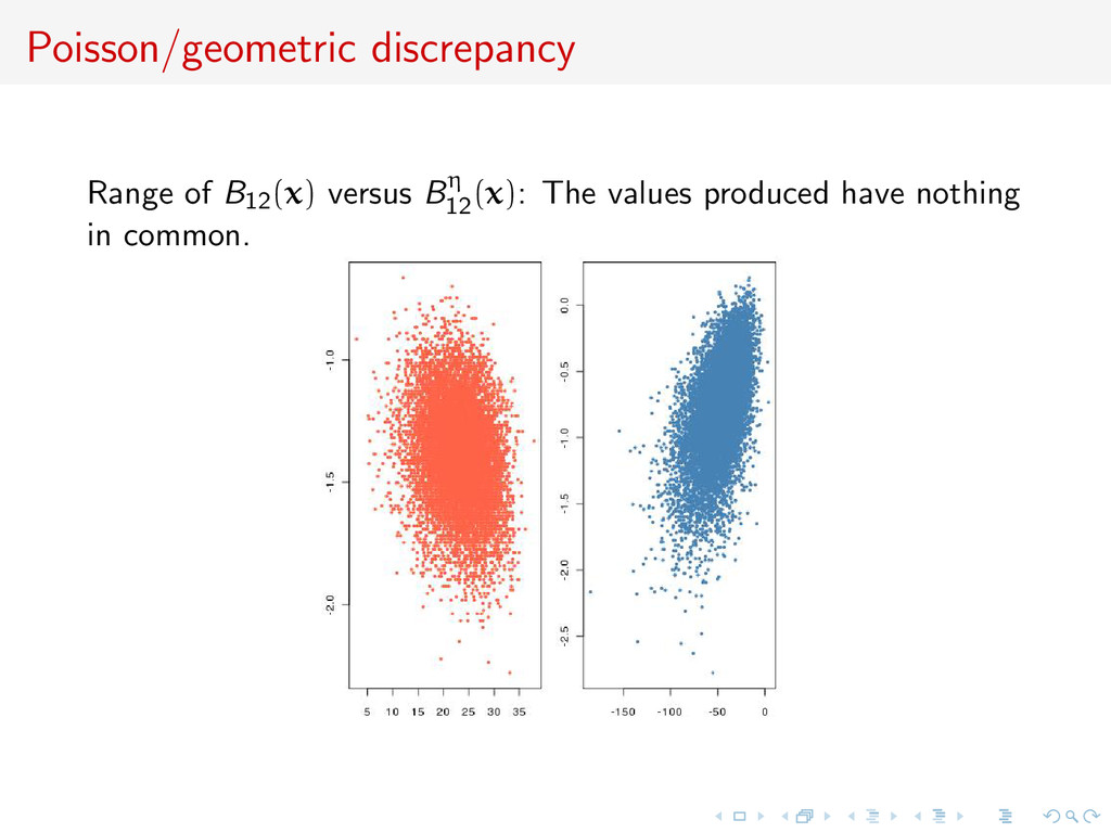
= T t=1 Imt =1 Iρ{η(zt ),η(y)} T t=1 Imt =2 Iρ{η(zt ),η(y)} , where the (mt, zt)’s are simulated from the (joint) prior As T goes to infinity, limit B12 (y) = Iρ{η(z),η(y)} π1(θ1)f1(z|θ1) dz dθ1 Iρ{η(z),η(y)} π2(θ2)f2(z|θ2) dz dθ2 = Iρ{η,η(y)} π1(θ1)f η 1 (η|θ1) dη dθ1 Iρ{η,η(y)} π2(θ2)f η 2 (η|θ2) dη dθ2 , where f η 1 (η|θ1) and f η 2 (η|θ2) distributions of η(z)
= T t=1 Imt =1 Iρ{η(zt ),η(y)} T t=1 Imt =2 Iρ{η(zt ),η(y)} , where the (mt, zt)’s are simulated from the (joint) prior As T goes to infinity, limit B12 (y) = Iρ{η(z),η(y)} π1(θ1)f1(z|θ1) dz dθ1 Iρ{η(z),η(y)} π2(θ2)f2(z|θ2) dz dθ2 = Iρ{η,η(y)} π1(θ1)f η 1 (η|θ1) dη dθ1 Iρ{η,η(y)} π2(θ2)f η 2 (η|θ2) dη dθ2 , where f η 1 (η|θ1) and f η 2 (η|θ2) distributions of η(z)
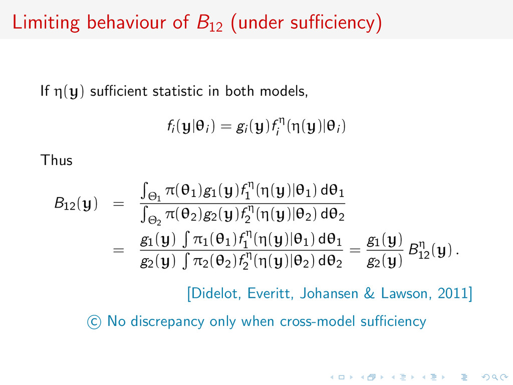
in both models, fi (y|θi ) = gi (y)f η i (η(y)|θi ) Thus B12(y) = Θ1 π(θ1)g1(y)f η 1 (η(y)|θ1) dθ1 Θ2 π(θ2)g2(y)f η 2 (η(y)|θ2) dθ2 = g1(y) π1(θ1)f η 1 (η(y)|θ1) dθ1 g2(y) π2(θ2)f η 2 (η(y)|θ2) dθ2 = g1(y) g2(y) Bη 12 (y) . [Didelot, Everitt, Johansen & Lawson, 2011] c No discrepancy only when cross-model sufficiency
in both models, fi (y|θi ) = gi (y)f η i (η(y)|θi ) Thus B12(y) = Θ1 π(θ1)g1(y)f η 1 (η(y)|θ1) dθ1 Θ2 π(θ2)g2(y)f η 2 (η(y)|θ2) dθ2 = g1(y) π1(θ1)f η 1 (η(y)|θ1) dθ1 g2(y) π2(θ2)f η 2 (η(y)|θ2) dθ2 = g1(y) g2(y) Bη 12 (y) . [Didelot, Everitt, Johansen & Lawson, 2011] c No discrepancy only when cross-model sufficiency
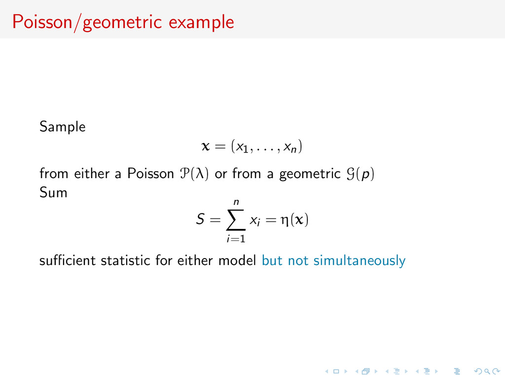
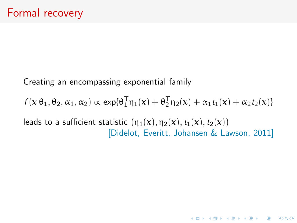
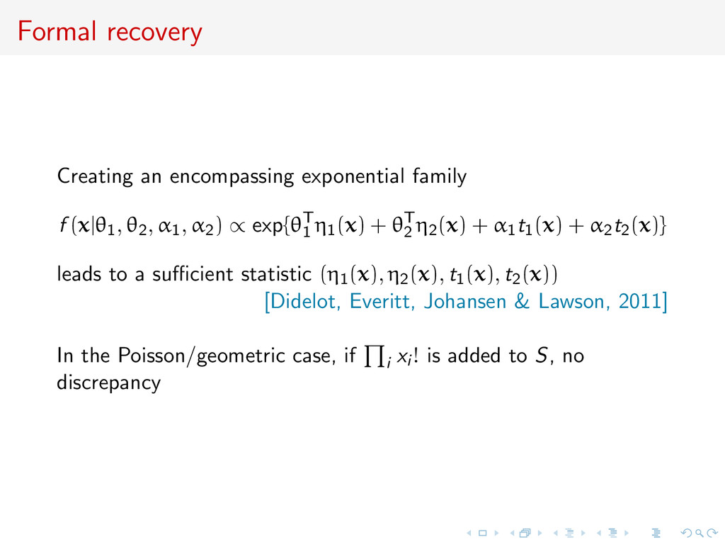
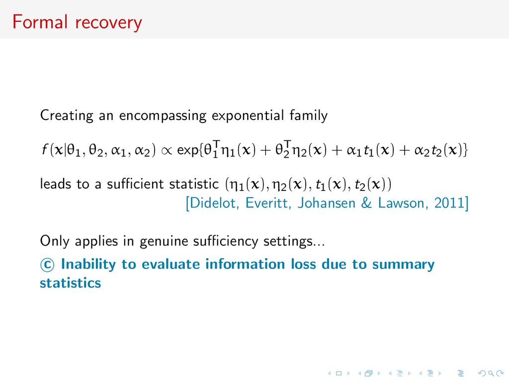
α1, α2) ∝ exp{θT 1 η1(x) + θT 2 η2(x) + α1t1(x) + α2t2(x)} leads to a sufficient statistic (η1(x), η2(x), t1(x), t2(x)) [Didelot, Everitt, Johansen & Lawson, 2011] In the Poisson/geometric case, if i xi ! is added to S, no discrepancy
α1, α2) ∝ exp{θT 1 η1(x) + θT 2 η2(x) + α1t1(x) + α2t2(x)} leads to a sufficient statistic (η1(x), η2(x), t1(x), t2(x)) [Didelot, Everitt, Johansen & Lawson, 2011] Only applies in genuine sufficiency settings... c Inability to evaluate information loss due to summary statistics
an inference machine ABC for model choice Model choice consistency Formalised framework Consistency results Summary statistics Conclusion and perspectives
for model choice: When is a Bayes factor based on an insufficient statistic T(y) consistent? Note/warnin: c drawn on T(y) through BT 12 (y) necessarily differs from c drawn on y through B12(y) [Marin, Pillai, X, & Rousseau, JRSS B, 2013]
for model choice: When is a Bayes factor based on an insufficient statistic T(y) consistent? Note/warnin: c drawn on T(y) through BT 12 (y) necessarily differs from c drawn on y through B12(y) [Marin, Pillai, X, & Rousseau, JRSS B, 2013]
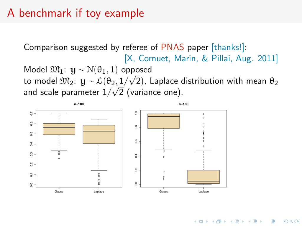
PNAS paper [thanks!]: [X, Cornuet, Marin, & Pillai, Aug. 2011] Model M1: y ∼ N(θ1, 1) opposed to model M2: y ∼ L(θ2, 1/ √ 2), Laplace distribution with mean θ2 and scale parameter 1/ √ 2 (variance one).
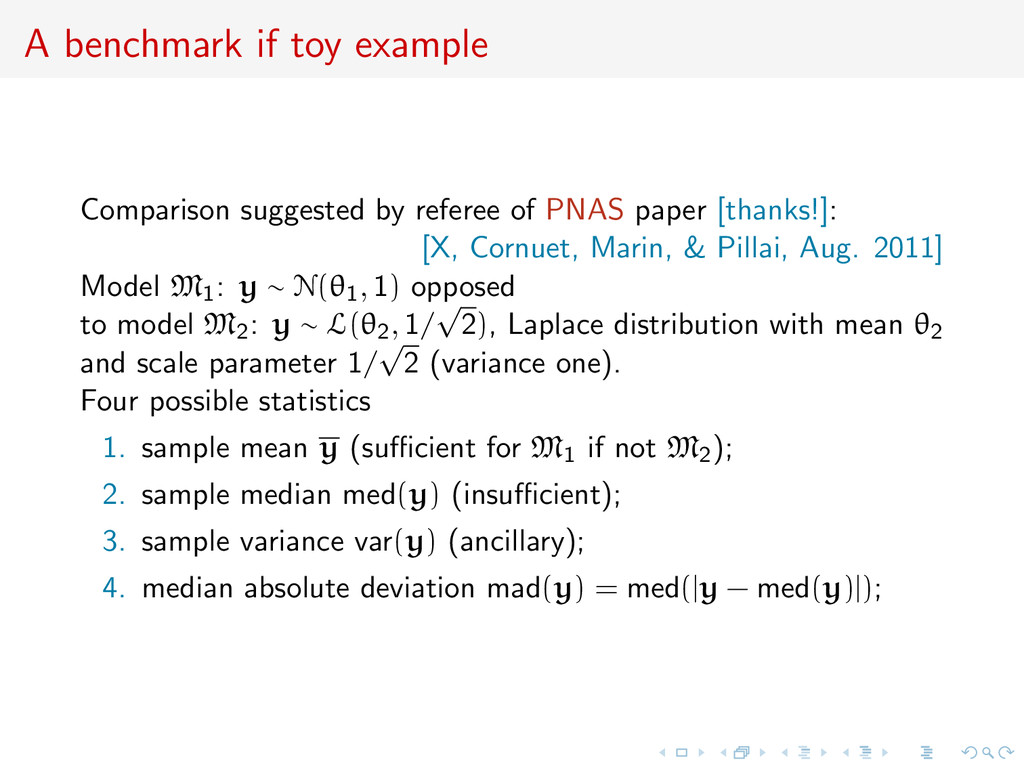
PNAS paper [thanks!]: [X, Cornuet, Marin, & Pillai, Aug. 2011] Model M1: y ∼ N(θ1, 1) opposed to model M2: y ∼ L(θ2, 1/ √ 2), Laplace distribution with mean θ2 and scale parameter 1/ √ 2 (variance one). Four possible statistics 1. sample mean y (sufficient for M1 if not M2); 2. sample median med(y) (insufficient); 3. sample variance var(y) (ancillary); 4. median absolute deviation mad(y) = med(|y − med(y)|);
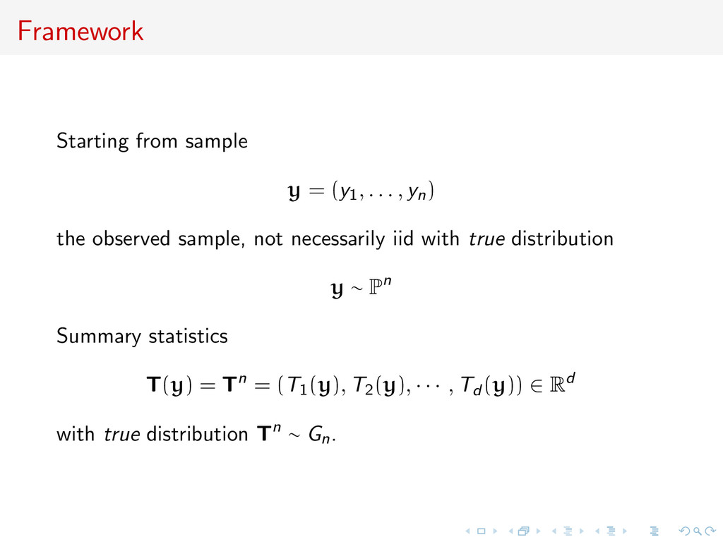
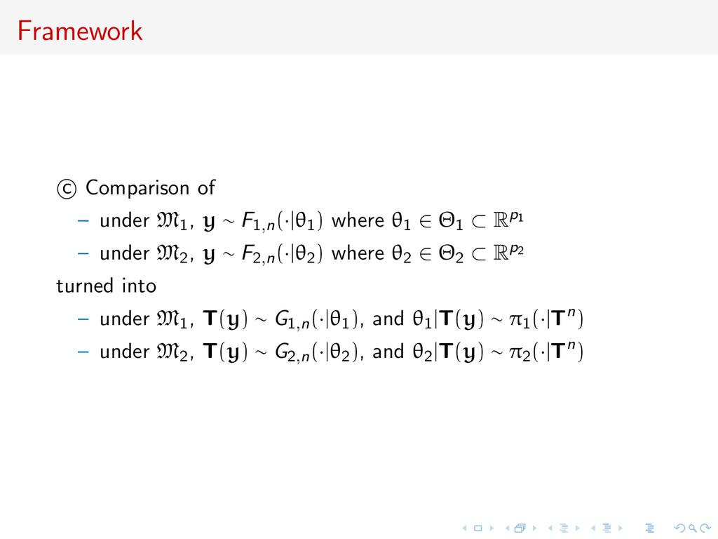
where θ1 ∈ Θ1 ⊂ Rp1 – under M2, y ∼ F2,n(·|θ2) where θ2 ∈ Θ2 ⊂ Rp2 turned into – under M1, T(y) ∼ G1,n(·|θ1), and θ1|T(y) ∼ π1(·|Tn) – under M2, T(y) ∼ G2,n(·|θ2), and θ2|T(y) ∼ π2(·|Tn)
standard central limit theorem under the true model [A2] controls the large deviations of the estimator Tn from the estimand µ(θ) [A3] is the standard prior mass condition found in Bayesian asymptotics (di effective dimension of the parameter) [A4] restricts the behaviour of the model density against the true density [Think CLT!]
There exist a sequence {vn} converging to +∞, a distribution Q, a symmetric, d × d positive definite matrix V0 and a vector µ0 ∈ Rd such that vnV −1/2 0 (Tn − µ0) n→∞ Q, under Gn
For i = 1, 2, there exist sets Fn,i ⊂ Θi , functions µi (θi ) and constants i , τi , αi > 0 such that for all τ > 0, sup θi ∈Fn,i Gi,n |Tn − µi (θi )| > τ|µi (θi ) − µ0| ∧ i |θi (|τµi (θi ) − µ0| ∧ i )−αi v−αi n with πi (Fc n,i ) = o(v−τi n ).
If inf{|µi (θi ) − µ0|; θi ∈ Θi } = 0, for any > 0, there exist U, δ > 0 and (En)n such that, if θi ∈ Sn,i (U) En ⊂ {t; gi (t|θi ) < δgn(t)} and Gn (Ec n ) < .
(sumup) [A1] is a standard central limit theorem under the true model [A2] controls the large deviations of the estimator Tn from the estimand µ(θ) [A3] is the standard prior mass condition found in Bayesian asymptotics (di effective dimension of the parameter) [A4] restricts the behaviour of the model density against the true density
− µ0|; θi ∈ Θi } = 0, mi (Tn) gn(Tn) ∼ v−di n , thus log(mi (Tn)/gn(Tn)) ∼ −di log vn and v−di n penalization factor resulting from integrating θi out (see effective number of parameters in DIC)
(t|θi ) πi (θi ) dθi is such that (i) if inf{|µi (θi ) − µ0|; θi ∈ Θi } = 0, Cl vd−di n mi (Tn) Cuvd−di n and (ii) if inf{|µi (θi ) − µ0|; θi ∈ Θi } > 0 mi (Tn) = oPn [vd−τi n + vd−αi n ].
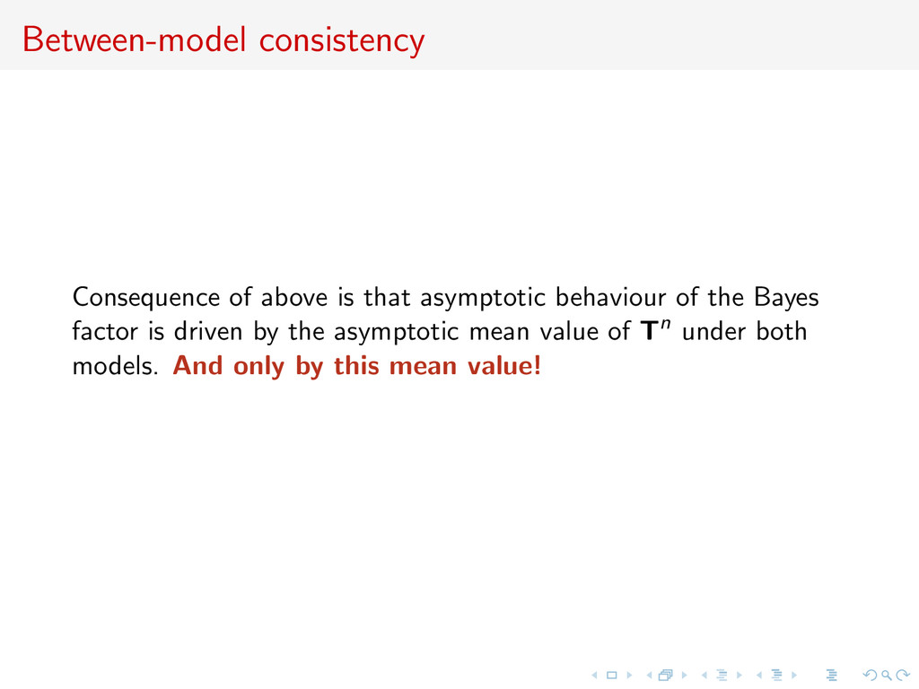
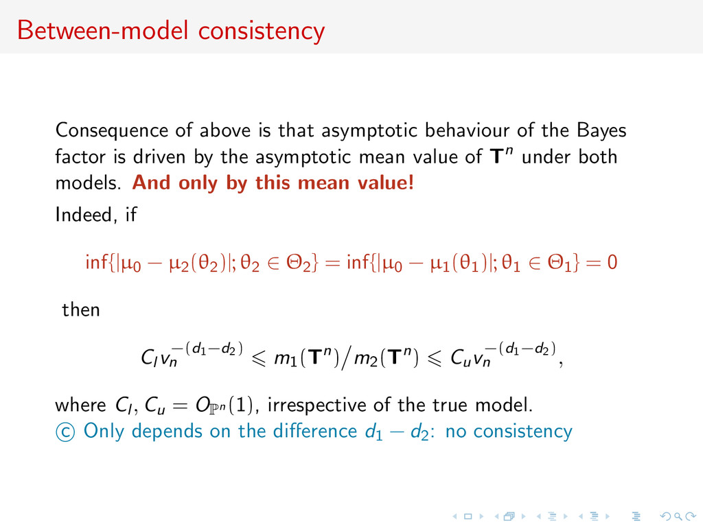
the Bayes factor is driven by the asymptotic mean value of Tn under both models. And only by this mean value! Indeed, if inf{|µ0 − µ2(θ2)|; θ2 ∈ Θ2} = inf{|µ0 − µ1(θ1)|; θ1 ∈ Θ1} = 0 then Cl v−(d1−d2) n m1(Tn) m2(Tn) Cuv−(d1−d2) n , where Cl , Cu = OPn (1), irrespective of the true model. c Only depends on the difference d1 − d2: no consistency
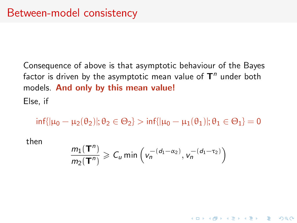
the Bayes factor is driven by the asymptotic mean value of Tn under both models. And only by this mean value! Else, if inf{|µ0 − µ2(θ2)|; θ2 ∈ Θ2} > inf{|µ0 − µ1(θ1)|; θ1 ∈ Θ1} = 0 then m1(Tn) m2(Tn) Cu min v−(d1−α2) n , v−(d1−τ2) n
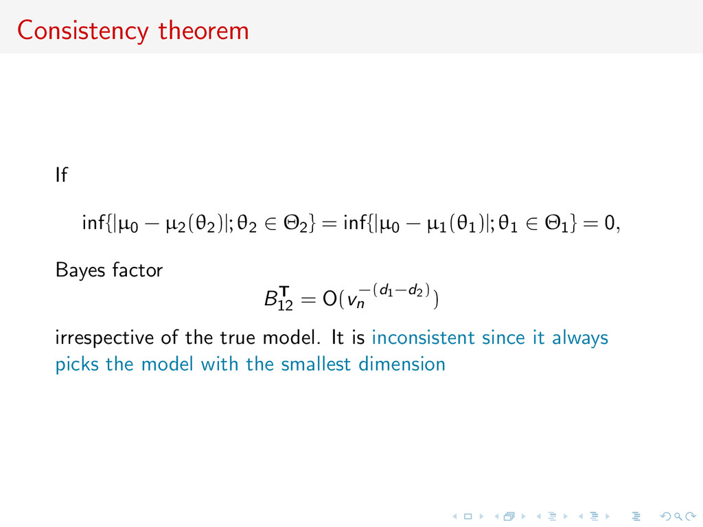
inf{|µ0 − µ1(θ1)|; θ1 ∈ Θ1} = 0, Bayes factor BT 12 = O(v−(d1−d2) n ) irrespective of the true model. It is inconsistent since it always picks the model with the smallest dimension
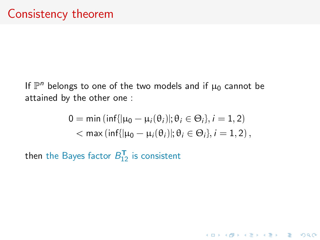
models and if µ0 cannot be attained by the other one : 0 = min (inf{|µ0 − µi (θi )|; θi ∈ Θi }, i = 1, 2) < max (inf{|µ0 − µi (θi )|; θi ∈ Θi }, i = 1, 2) , then the Bayes factor BT 12 is consistent
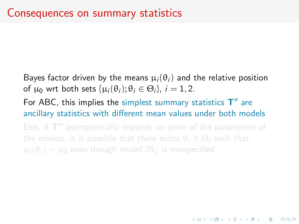
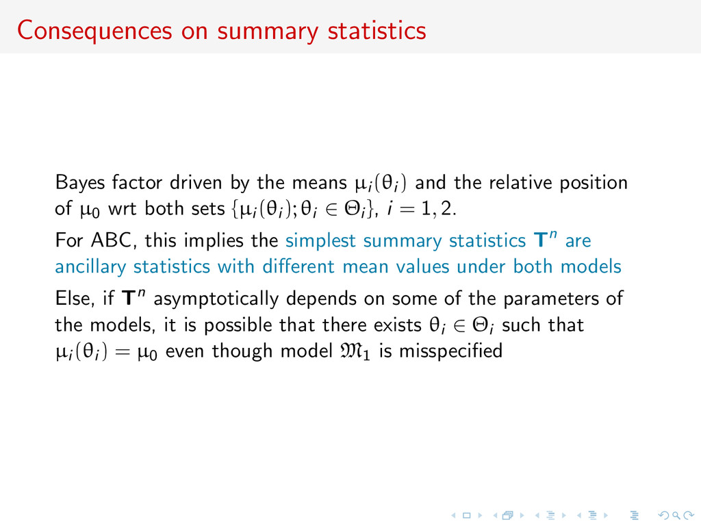
µi (θi ) and the relative position of µ0 wrt both sets {µi (θi ); θi ∈ Θi }, i = 1, 2. For ABC, this implies the simplest summary statistics Tn are ancillary statistics with different mean values under both models Else, if Tn asymptotically depends on some of the parameters of the models, it is possible that there exists θi ∈ Θi such that µi (θi ) = µ0 even though model M1 is misspecified
µi (θi ) and the relative position of µ0 wrt both sets {µi (θi ); θi ∈ Θi }, i = 1, 2. For ABC, this implies the simplest summary statistics Tn are ancillary statistics with different mean values under both models Else, if Tn asymptotically depends on some of the parameters of the models, it is possible that there exists θi ∈ Θi such that µi (θi ) = µ0 even though model M1 is misspecified
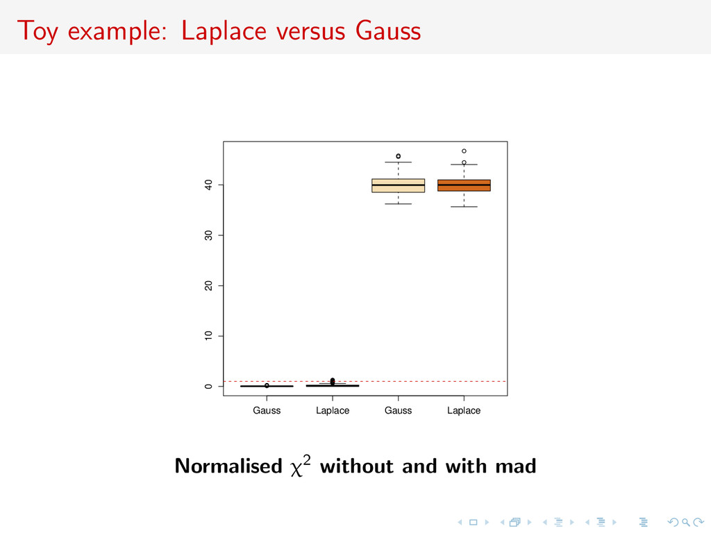
n i=1 X4 i , µ1(θ) = 3 + θ4 + 6θ2, µ2(θ) = 6 + · · · and the true distribution is Laplace with mean θ0 = 1, under the Gaussian model the value θ∗ = 2 √ 3 − 3 also leads to µ0 = µ(θ∗) [here d1 = d2 = d = 1]
n i=1 X4 i , µ1(θ) = 3 + θ4 + 6θ2, µ2(θ) = 6 + · · · and the true distribution is Laplace with mean θ0 = 1, under the Gaussian model the value θ∗ = 2 √ 3 − 3 also leads to µ0 = µ(θ∗) [here d1 = d2 = d = 1] c A Bayes factor associated with such a statistic is inconsistent
y(4) n , ¯ y(6) n and the true distribution is Laplace with mean θ0 = 0, then µ0 = 6, µ1(θ∗ 1 ) = 6 with θ∗ 1 = 2 √ 3 − 3 [d1 = 1 and d2 = 1/2] thus B12 ∼ n−1/4 → 0 : consistent Under the Gaussian model µ0 = 3, µ2(θ2) 6 > 3 ∀θ2 B12 → +∞ : consistent
y(4) n , ¯ y(6) n and the true distribution is Laplace with mean θ0 = 0, then µ0 = 6, µ1(θ∗ 1 ) = 6 with θ∗ 1 = 2 √ 3 − 3 [d1 = 1 and d2 = 1/2] thus B12 ∼ n−1/4 → 0 : consistent Under the Gaussian model µ0 = 3, µ2(θ2) 6 > 3 ∀θ2 B12 → +∞ : consistent
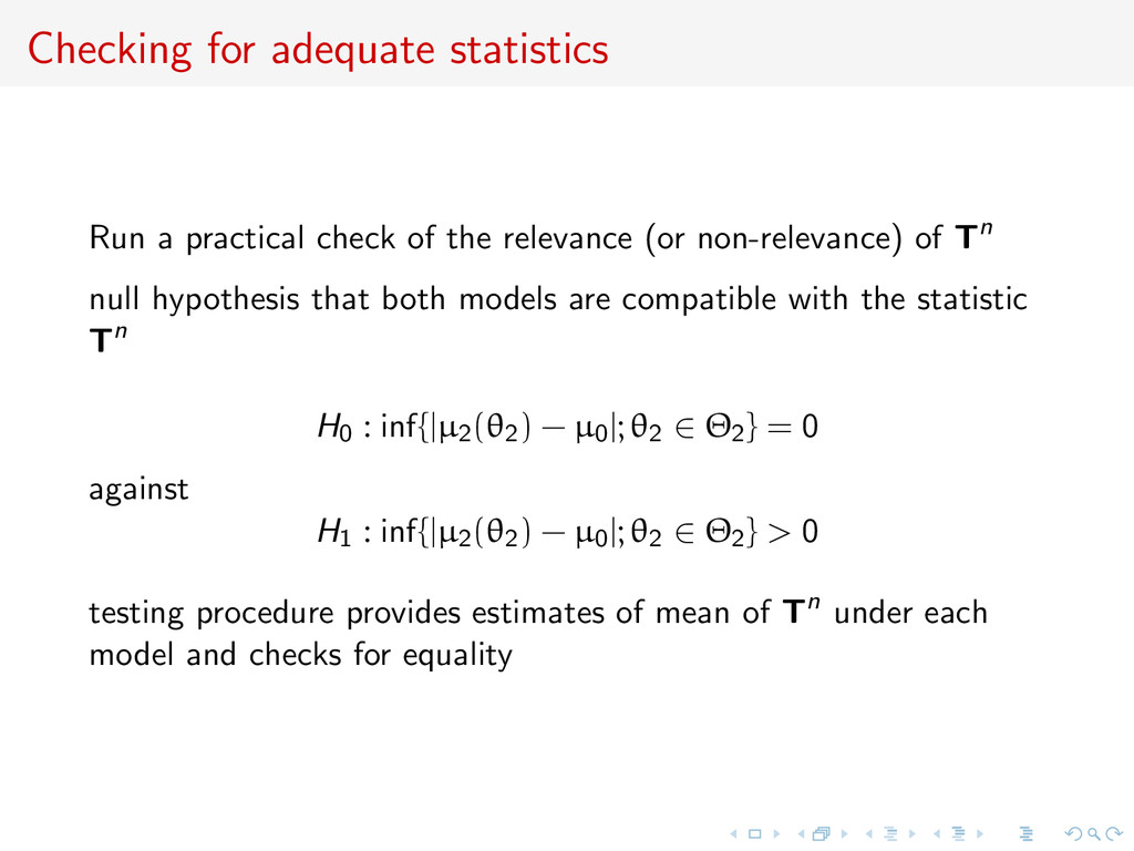
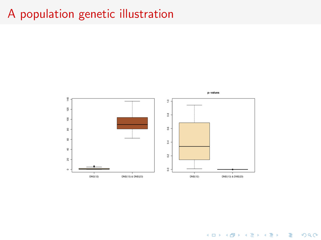
relevance (or non-relevance) of Tn null hypothesis that both models are compatible with the statistic Tn H0 : inf{|µ2(θ2) − µ0|; θ2 ∈ Θ2} = 0 against H1 : inf{|µ2(θ2) − µ0|; θ2 ∈ Θ2} > 0 testing procedure provides estimates of mean of Tn under each model and checks for equality
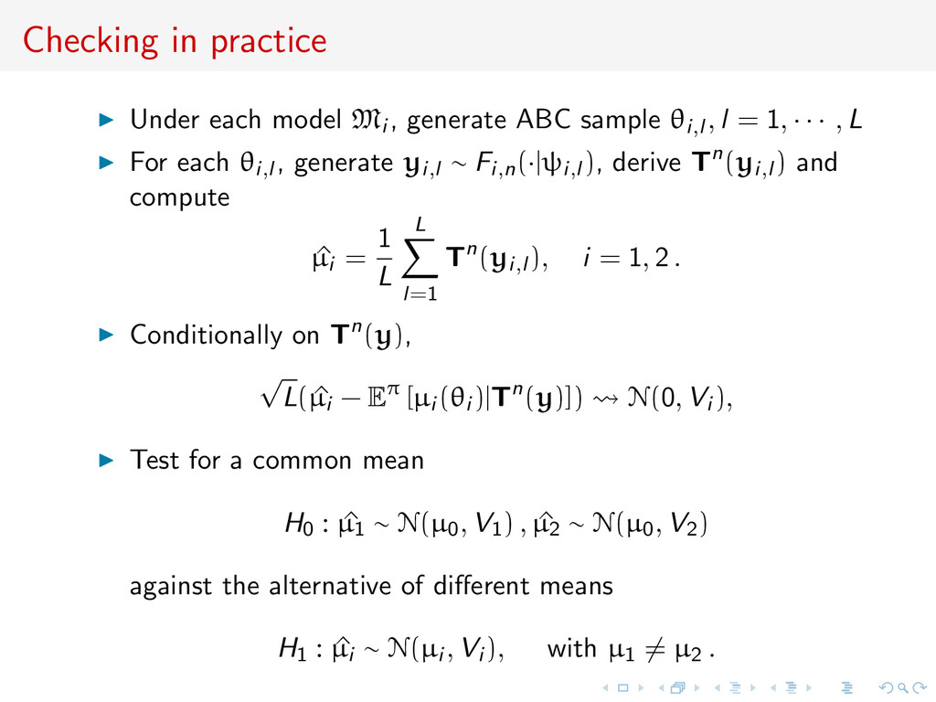
sample θi,l , l = 1, · · · , L For each θi,l , generate yi,l ∼ Fi,n(·|ψi,l ), derive Tn(yi,l ) and compute ^ µi = 1 L L l=1 Tn(yi,l ), i = 1, 2 . Conditionally on Tn(y), √ L( ^ µi − Eπ [µi (θi )|Tn(y)]) N(0, Vi ), Test for a common mean H0 : ^ µ1 ∼ N(µ0, V1) , ^ µ2 ∼ N(µ0, V2) against the alternative of different means H1 : ^ µi ∼ N(µi , Vi ), with µ1 = µ2 .
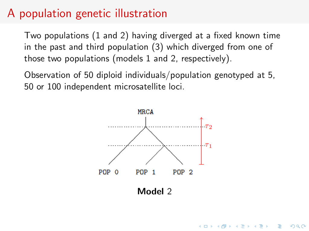
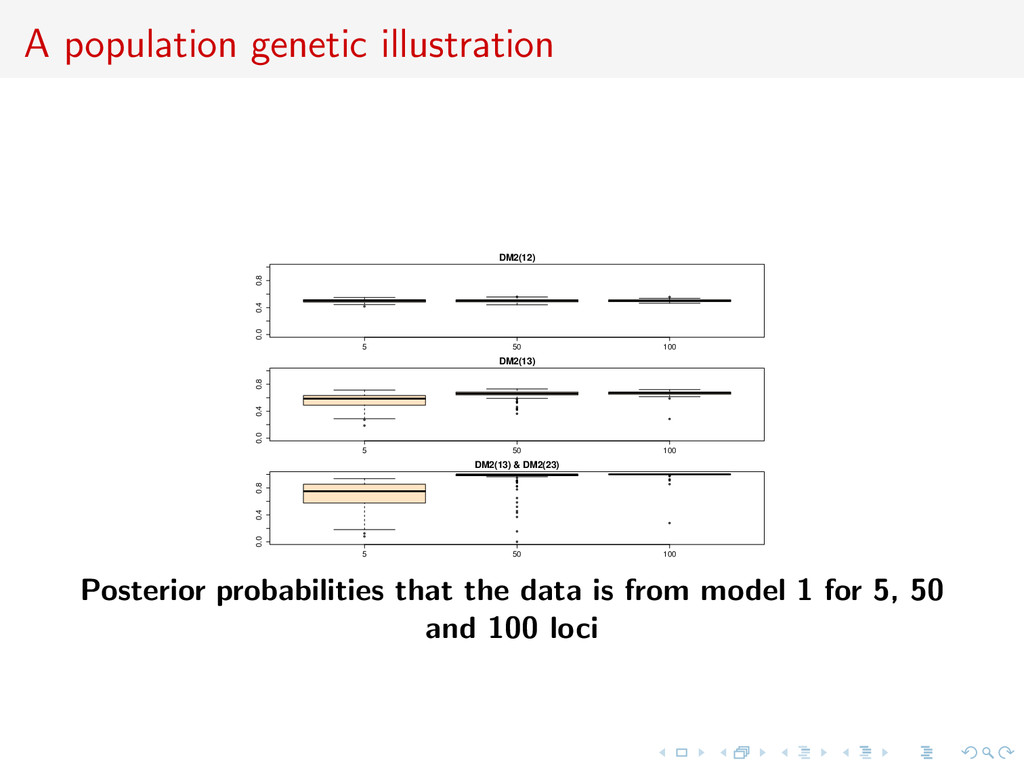
diverged at a fixed known time in the past and third population (3) which diverged from one of those two populations (models 1 and 2, respectively). Observation of 50 diploid individuals/population genotyped at 5, 50 or 100 independent microsatellite loci. Model 2
diverged at a fixed known time in the past and third population (3) which diverged from one of those two populations (models 1 and 2, respectively). Observation of 50 diploid individuals/population genotyped at 5, 50 or 100 independent microsatellite loci. Stepwise mutation model: the number of repeats of the mutated gene increases or decreases by one. Mutation rate µ common to all loci set to 0.005 (single parameter) with uniform prior distribution µ ∼ U[0.0001, 0.01]
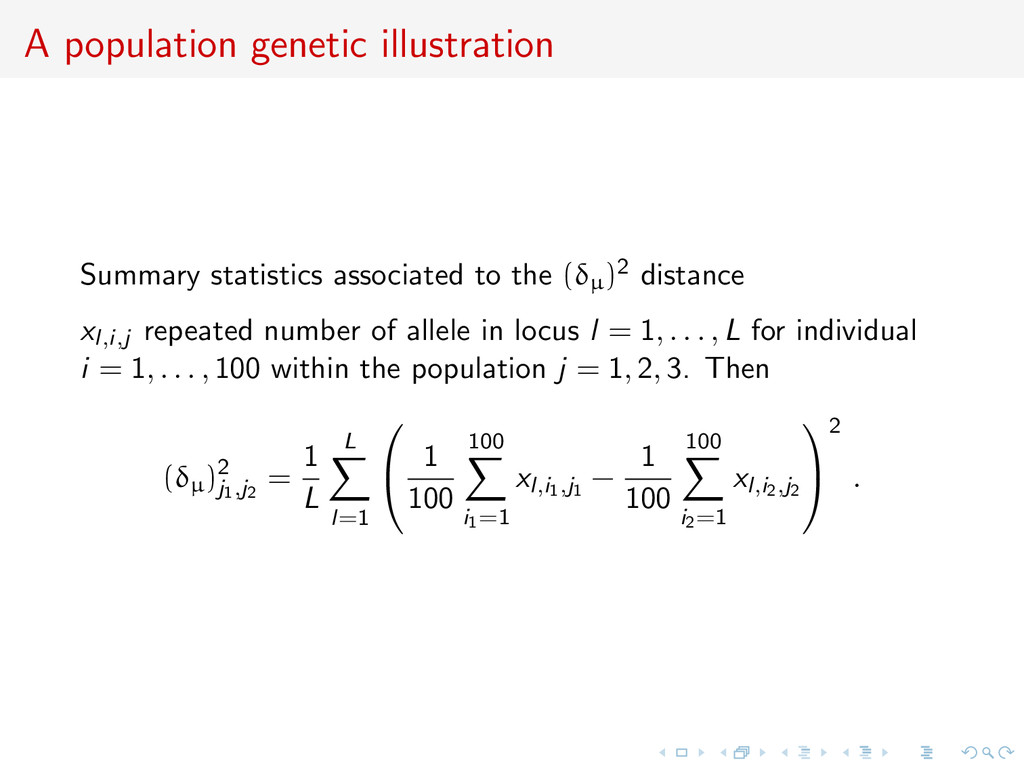
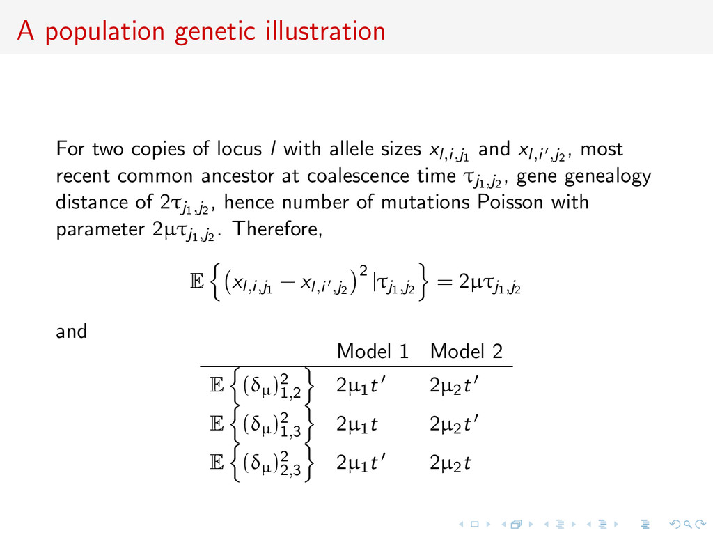
distance xl,i,j repeated number of allele in locus l = 1, . . . , L for individual i = 1, . . . , 100 within the population j = 1, 2, 3. Then (δµ)2 j1,j2 = 1 L L l=1 1 100 100 i1=1 xl,i1,j1 − 1 100 100 i2=1 xl,i2,j2 2 .
with allele sizes xl,i,j1 and xl,i ,j2 , most recent common ancestor at coalescence time τj1,j2 , gene genealogy distance of 2τj1,j2 , hence number of mutations Poisson with parameter 2µτj1,j2 . Therefore, E xl,i,j1 − xl,i ,j2 2 |τj1,j2 = 2µτj1,j2 and Model 1 Model 2 E (δµ)2 1,2 2µ1t 2µ2t E (δµ)2 1,3 2µ1t 2µ2t E (δµ)2 2,3 2µ1t 2µ2t
distance (δµ)2 1,2 not convergent: if µ1 = µ2, same expectation Bayes factor based only on distance (δµ)2 1,3 or (δµ)2 2,3 not convergent: if µ1 = 2µ2 or 2µ1 = µ2 same expectation if two of the three distances are used, Bayes factor converges: there is no (µ1, µ2) for which all expectations are equal
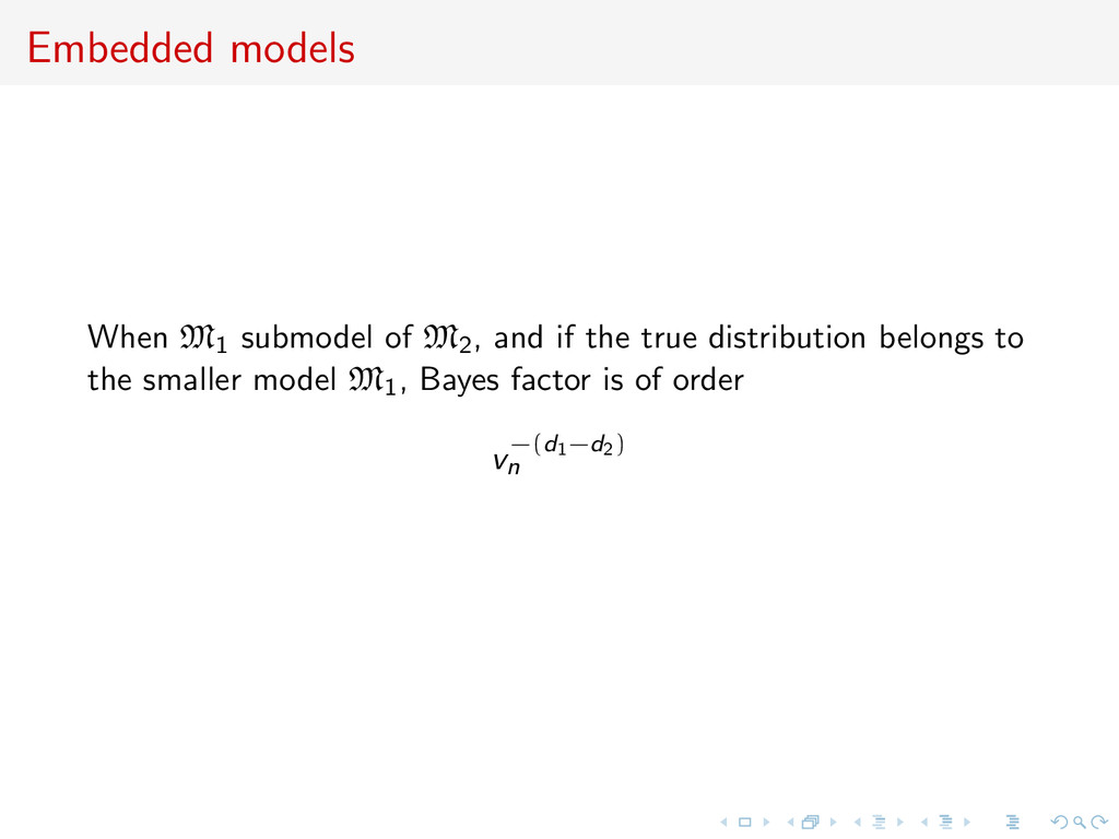
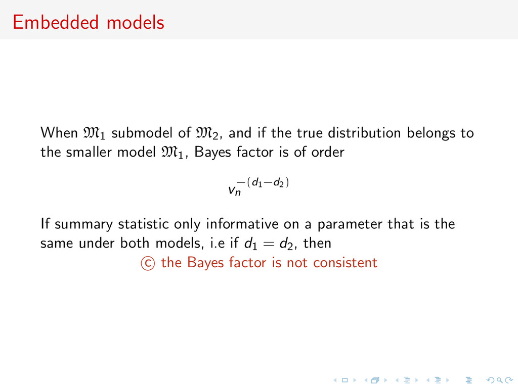
true distribution belongs to the smaller model M1, Bayes factor is of order v−(d1−d2) n If summary statistic only informative on a parameter that is the same under both models, i.e if d1 = d2, then c the Bayes factor is not consistent
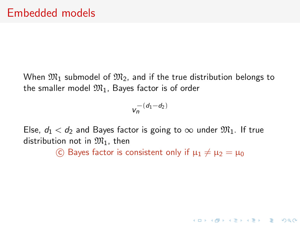
true distribution belongs to the smaller model M1, Bayes factor is of order v−(d1−d2) n Else, d1 < d2 and Bayes factor is going to ∞ under M1. If true distribution not in M1, then c Bayes factor is consistent only if µ1 = µ2 = µ0
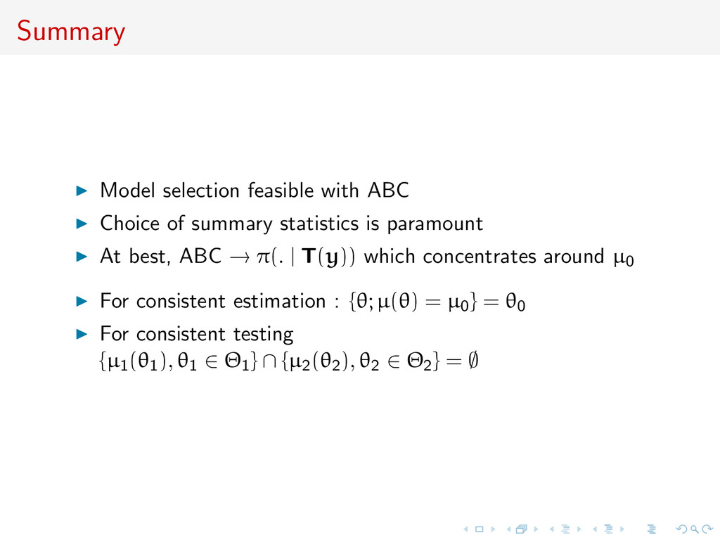
Data models, able to start from rudimentary machine learning summaries many formats of empirical [likelihood] Bayes methods available lack of comparative tools and of an assessment for information loss
![Different [levels of] worries about abc Impact on B inference](https://files.speakerdeck.com/presentations/93e87030242901315d54262c2bebb983/slide_8.jpg)
![Different [levels of] worries about abc Impact on B inference](https://files.speakerdeck.com/presentations/93e87030242901315d54262c2bebb983/slide_9.jpg)
![Different [levels of] worries about abc Impact on B inference](https://files.speakerdeck.com/presentations/93e87030242901315d54262c2bebb983/slide_10.jpg)
![A?B?C? A stands for approximate [wrong likelihood / pic?] B](https://files.speakerdeck.com/presentations/93e87030242901315d54262c2bebb983/slide_24.jpg)
![A?B?C? A stands for approximate [wrong likelihood / pic?] B](https://files.speakerdeck.com/presentations/93e87030242901315d54262c2bebb983/slide_25.jpg)
![A?B?C? A stands for approximate [wrong likelihood / pic?] B](https://files.speakerdeck.com/presentations/93e87030242901315d54262c2bebb983/slide_26.jpg)
![ABC as knn [Biau et al., 2013, Annales de l’IHP]](https://files.speakerdeck.com/presentations/93e87030242901315d54262c2bebb983/slide_44.jpg)
![ABC as knn [Biau et al., 2013, Annales de l’IHP]](https://files.speakerdeck.com/presentations/93e87030242901315d54262c2bebb983/slide_45.jpg)
![ABC as knn [Biau et al., 2013, Annales de l’IHP]](https://files.speakerdeck.com/presentations/93e87030242901315d54262c2bebb983/slide_46.jpg)
![Summary [of F&P/statistics) optimality of the posterior expectation E[θ|y] of](https://files.speakerdeck.com/presentations/93e87030242901315d54262c2bebb983/slide_64.jpg)
![Summary [of F&P/statistics) optimality of the posterior expectation E[θ|y] of](https://files.speakerdeck.com/presentations/93e87030242901315d54262c2bebb983/slide_65.jpg)
![Assumptions A collection of asymptotic “standard” assumptions: [A1] is a](https://files.speakerdeck.com/presentations/93e87030242901315d54262c2bebb983/slide_109.jpg)
![Assumptions A collection of asymptotic “standard” assumptions: [Think CLT!] [A1]](https://files.speakerdeck.com/presentations/93e87030242901315d54262c2bebb983/slide_110.jpg)
![Assumptions A collection of asymptotic “standard” assumptions: [Think CLT!] [A2]](https://files.speakerdeck.com/presentations/93e87030242901315d54262c2bebb983/slide_111.jpg)
![Assumptions A collection of asymptotic “standard” assumptions: [Think CLT!] [A3]](https://files.speakerdeck.com/presentations/93e87030242901315d54262c2bebb983/slide_112.jpg)
![Assumptions A collection of asymptotic “standard” assumptions: [Think CLT!] [A4]](https://files.speakerdeck.com/presentations/93e87030242901315d54262c2bebb983/slide_113.jpg)
![Assumptions A collection of asymptotic “standard” assumptions: [Think CLT!] Again](https://files.speakerdeck.com/presentations/93e87030242901315d54262c2bebb983/slide_114.jpg)
![Effective dimension Understanding di in [A3]: defined only when µ0](https://files.speakerdeck.com/presentations/93e87030242901315d54262c2bebb983/slide_115.jpg)
![Effective dimension Understanding di in [A3]: when inf{|µi (θi )](https://files.speakerdeck.com/presentations/93e87030242901315d54262c2bebb983/slide_116.jpg)
![Effective dimension Understanding di in [A3]: In regular models, di](https://files.speakerdeck.com/presentations/93e87030242901315d54262c2bebb983/slide_117.jpg)
![Asymptotic marginals Asymptotically, under [A1]–[A4] mi (t) = Θi gi](https://files.speakerdeck.com/presentations/93e87030242901315d54262c2bebb983/slide_118.jpg)
![Toy example: Laplace versus Gauss [1] If Tn = n−1](https://files.speakerdeck.com/presentations/93e87030242901315d54262c2bebb983/slide_127.jpg)
![Toy example: Laplace versus Gauss [1] If Tn = n−1](https://files.speakerdeck.com/presentations/93e87030242901315d54262c2bebb983/slide_128.jpg)
![Toy example: Laplace versus Gauss [1] If Tn = n−1](https://files.speakerdeck.com/presentations/93e87030242901315d54262c2bebb983/slide_129.jpg)
![Toy example: Laplace versus Gauss [1] If Tn = n−1](https://files.speakerdeck.com/presentations/93e87030242901315d54262c2bebb983/slide_130.jpg)
![Toy example: Laplace versus Gauss [0] When T(y) = ¯](https://files.speakerdeck.com/presentations/93e87030242901315d54262c2bebb983/slide_131.jpg)
![Toy example: Laplace versus Gauss [0] When T(y) = ¯](https://files.speakerdeck.com/presentations/93e87030242901315d54262c2bebb983/slide_132.jpg)
![Toy example: Laplace versus Gauss [0] When T(y) = ¯](https://files.speakerdeck.com/presentations/93e87030242901315d54262c2bebb983/slide_133.jpg)