Shape identification in non-linear inverse problems

Transcript

1. Shape identification in nonlinear inverse problems Han Wang1 Department of Mathematics and Applications Ecole Normale Sup´ erieure, Paris www.math.ens.fr/~hanwang Groupe de travail M´ ethodes Num´ eriques Laboratoire Jacques-Louis Lions, UPMC April 28, 2014 1 Joint work with H.Ammari, T.Boulier, J.Chen, Z.Chen, D.Chung, J.Garnier, W.Jing, H.Kang, S.Mallat, M.P.Tran, D.Volkov, I.Waldspurger 1
2. Active electrolocation and echolocation in the nature (a) Elephant nose fish (b) Brown long-eared bat Generate and detect electric/acoustic fields Locate and identify targets: position, material composition and shape 2
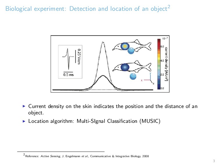
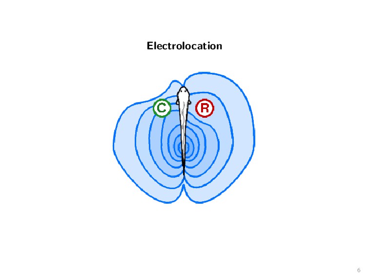
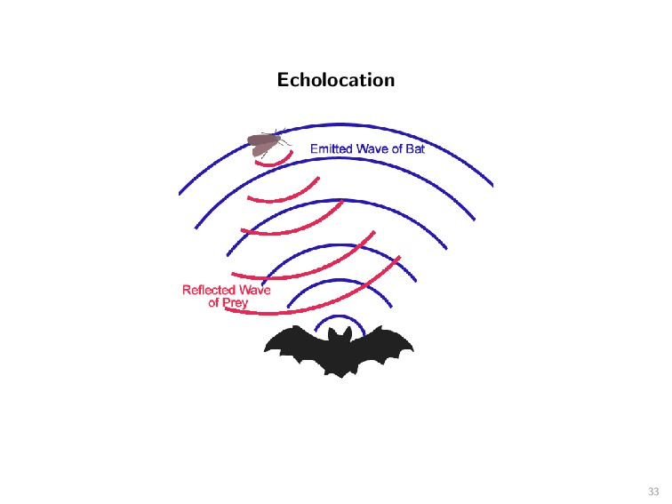
3. Biological experiment: Detection and location of an object2 Current density on the skin indicates the position and the distance of an object. Location algorithm: Multi-SIgnal Classification (MUSIC) 2 Reference: Active Sensing, J. Engelmann et al., Communicative & Integrative Biology, 2008 3
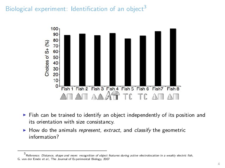
4. Biological experiment: Identification of an object3 Fish can be trained to identify an object independently of its position and its orientation with size consistancy. How do the animals represent, extract, and classify the geometric information? 3 Reference: Distance, shape and more: recognition of object features during active electrolocation in a weakly electric fish, G. von der Emde et al., The Journal of Experimental Biology, 2007 4
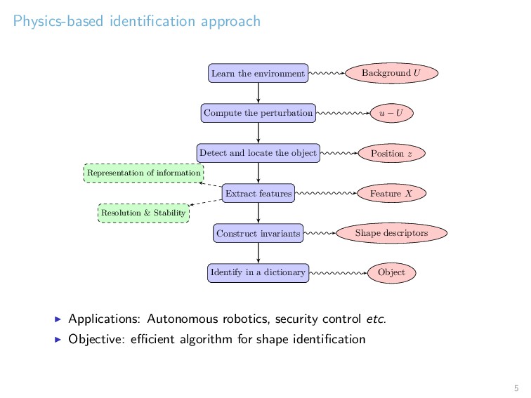
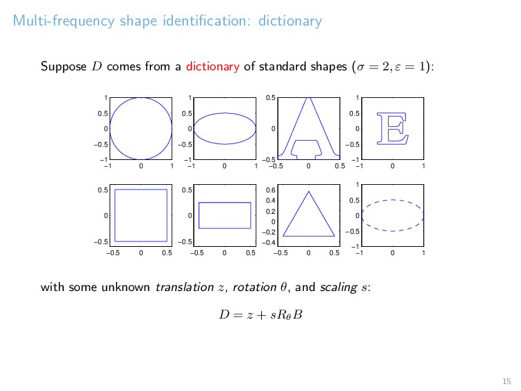
5. Physics-based identification approach Learn the environment Background U Compute the perturbation u − U Detect and locate the object Position z Extract features Feature X Construct invariants Shape descriptors Identify in a dictionary Object Representation of information Resolution & Stability Applications: Autonomous robotics, security control etc. Objective: efficient algorithm for shape identification 5
6. Electrolocation 6
7. Wave form Pulse type and wave type fish Electric organ discharge: Governing equation: ∇.(σ(x) + ε(x)∂t)∇u(t, x) = f(t, x), t ≥ 0 σ(x), ε(x): Conductivity and permittivity map u(t, x): electric potential f(t, x) = ˜ f(x)h(t): separable source, ˜ f: dipole 7
8. Electrolocation of wave type fish4 Source term is time periodic: f(x, t) = ˜ f(x) k akeitkω0 Ω: fish’s body, D: target located at z σ, ε: conductivity and permittivity of D, σ = 1. κ = σ + iεω: admittivity of D, ω = kω0: the probing frequency u : electric potential field generated by the fish at the frequency kω0:                            ∆u(x) = ˜ f(x), x ∈ Ω, ∇ · (1 + (κ − 1)χD)∇u(x) = 0, x ∈ Rd \ Ω, ∂u ∂ν (x) − = 0, x ∈ ∂Ω, u(x) + − u(x) − = ξ ∂u ∂ν (x) + , x ∈ ∂Ω, |u(x)| = O(|x|−d+1), |x| → ∞. Superposition principle for multiple frequency. Background filed U satisfies the same equation without D. 4 Modeling active electrolocation in weakly electric fish, T.Boulier et al., SIAM Journal on Imaging Sciences, 2013 8
9. Perturbation of the potential field ξ = 0.01, δ = 0.5, σ = 2, ε = 0: −1.5 −1 −0.5 0 0.5 1 1.5 −1.5 −1 −0.5 0 0.5 1 1.5 −10 −5 0 5 10 (c) Background field U −1.5 −1 −0.5 0 0.5 1 1.5 −1.5 −1 −0.5 0 0.5 1 1.5 −10 −5 0 5 10 (d) Field u with an object −1.5 −1 −0.5 0 0.5 1 1.5 −1.5 −1 −0.5 0 0.5 1 1.5 −0.06 −0.04 −0.02 0 0.02 0.04 0.06 (e) Perturbation u − U Dipole approximation: Dipole moment u(x) − U(x) ∇U(z) · M(κ, D) · ∇G(x − z) Polarization Tensor z: position of the object 9
10. Dipole approximation: ∇U(z) · M(κ, D) · ∇G(x − z) Polarization tensor (2-by-2 symmetric matrix): M(κ, D) := ∂D y(λI − K∗ D )−1 [ν](y) dσ(y), K∗ D [ϕ](x) = 1 ωd ∂D x − y, νx |x − y|d ϕ(y) dσ(y) , x ∈ ∂D λ = κ+1 2(κ−1) , κ = σ + iεω: admittivity contrast Spectrum of K∗ D is in (−1/2, 1/2], hence (λI − K∗ D ) is invertible. G: the Green function associated to Robin boundary conditions: for z ∈ R2 \ Ω,                ∆xG(x, z) = δz(x), x ∈ R2 \ Ω, G|+ − ξ ∂G ∂ν(x) + = 0, x ∈ ∂Ω, G − 1 2π log |x| = O(|x|−1), |x| → ∞. 10
11. Space-frequency response matrix Movement: fish takes measurement at different positions around the target −1 0 1 −1.5 −1 −0.5 0 0.5 1 1.5 −3 −2 −1 0 1 2 3 −1 0 1 −1.5 −1 −0.5 0 0.5 1 1.5 −3 −2 −1 0 1 2 3 −1 0 1 −1.5 −1 −0.5 0 0.5 1 1.5 −3 −2 −1 0 1 2 3 −1 0 1 −1.5 −1 −0.5 0 0.5 1 1.5 −3 −2 −1 0 1 2 3 Space-frequency response matrix: u electric potential field at kω0 V k sr = ∂u ∂ν (xr) + − ∂U ∂ν (xr) + , xs: position of the electric organ, (xr): receptors on the skin of the fish. 11
12. Space-frequency location algorithm V k sr ∇U(z) · ∝Id M(κ, D) · ∇ ∂G ∂νx (xr − z) Define the vector, z in the search domain, ˜ g(z ) := ∇U(z ) · ∇ ∂G ∂νx (x1 − z ), . . . , ∇U(z ) · ∇ ∂G ∂νx (xL − z ) T , and its normalized version g = ˜ g/|˜ g|. Imaging functional has a large peak at z: I(z ) := 1 |(Id −P)g(z )| , P: the orthogonal projection onto the first singular vector of the space-frequency response matrix Vs = (V k sr )rk. 12
13. Space-frequency location algorithm Detection of a small disk with the Space-frequency location algorithm: −1 −0.5 0 0.5 1 −0.2 0 0.2 0.4 0.6 0.8 1 1.2 1.4 1.6 0 50 100 150 200 0 0.1 0.2 0.3 0.4 0.5 0.6 0.7 0.8 0.9 1 0.5 0.6 0.7 0.8 0.9 1 1.1 1.2 1.3 1.4 1.5 50 100 150 200 250 Figure : Number of frequencies: 10. Number of receptors on the fish: 64. σ, ε can be determined by minimizing a quadratic misfit functional. 13
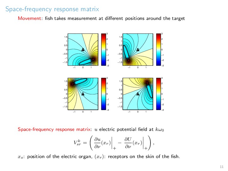
14. Feature extraction Mk := M(κ, D), κ = σ + iεkω0. We have the linear system: V k sr = ∂u ∂ν + − ∂U ∂ν + (xr) ∇U(z) · Mk · ∂G ∂νx (xr − z) L(Mk)sr Reconstruct Mk from V k by solving the least square problem: Mk = arg min M L(M) − V k L depends only on the postions of xs, xr Well conditioned system for full aperture and equally distributed xs, xr Inversion of L: very cheap operation – Post-processing on V by 1 2 I − K∗ Ω − ξ ∂DΩ ∂ν to convert the Green function of Robin boundary condition – Take imaginary part to eliminate the background field U 14
15. Multi-frequency shape identification: dictionary Suppose D comes from a dictionary of standard shapes (σ = 2, ε = 1): −1 0 1 −1 −0.5 0 0.5 1 −1 0 1 −1 −0.5 0 0.5 1 −0.5 0 0.5 −0.5 0 0.5 −1 0 1 −1 −0.5 0 0.5 1 −0.5 0 0.5 −0.5 0 0.5 −0.5 0 0.5 −0.5 0 0.5 −0.5 0 0.5 −0.4 −0.2 0 0.2 0.4 0.6 −1 0 1 −1 −0.5 0 0.5 1 with some unknown translation z, rotation θ, and scaling s: D = z + sRθ B 15
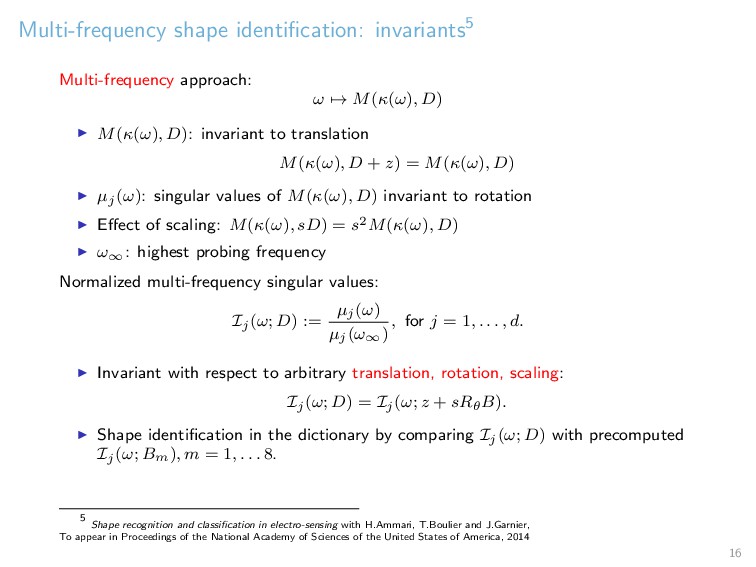
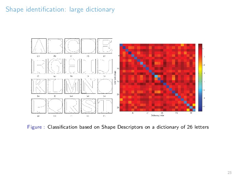
16. Multi-frequency shape identification: invariants5 Multi-frequency approach: ω → M(κ(ω), D) M(κ(ω), D): invariant to translation M(κ(ω), D + z) = M(κ(ω), D) µj(ω): singular values of M(κ(ω), D) invariant to rotation Effect of scaling: M(κ(ω), sD) = s2M(κ(ω), D) ω∞: highest probing frequency Normalized multi-frequency singular values: Ij(ω; D) := µj(ω) µj(ω∞) , for j = 1, . . . , d. Invariant with respect to arbitrary translation, rotation, scaling: Ij(ω; D) = Ij(ω; z + sRθB). Shape identification in the dictionary by comparing Ij(ω; D) with precomputed Ij(ω; Bm), m = 1, . . . 8. 5 Shape recognition and classification in electro-sensing with H.Ammari, T.Boulier and J.Garnier, To appear in Proceedings of the National Academy of Sciences of the United States of America, 2014 16
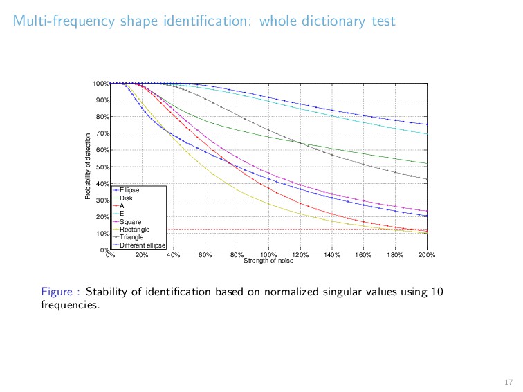
17. Multi-frequency shape identification: whole dictionary test 0% 20% 40% 60% 80% 100% 120% 140% 160% 180% 200% 0% 10% 20% 30% 40% 50% 60% 70% 80% 90% 100% Strength of noise Probability of detection Ellipse Disk A E Square Rectangle Triangle Different ellipse Figure : Stability of identification based on normalized singular values using 10 frequencies. 17
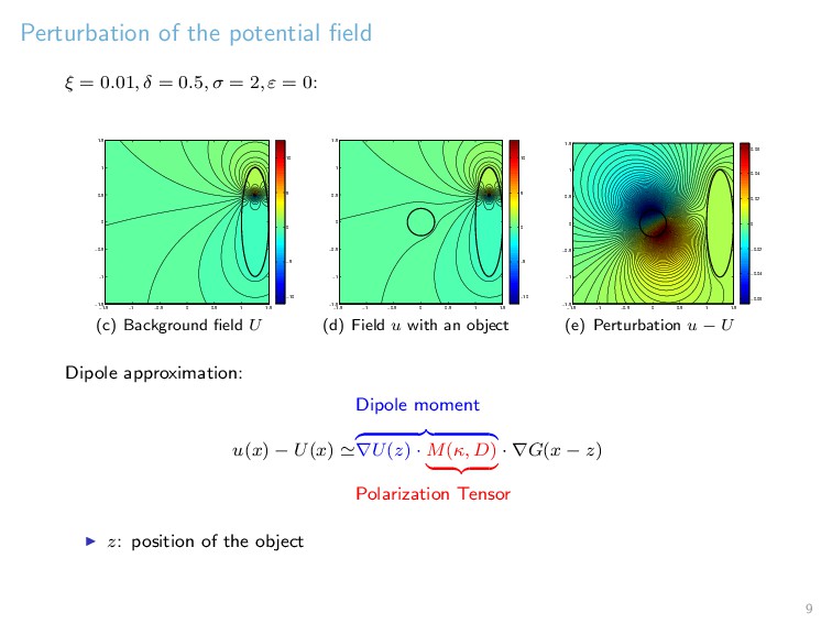
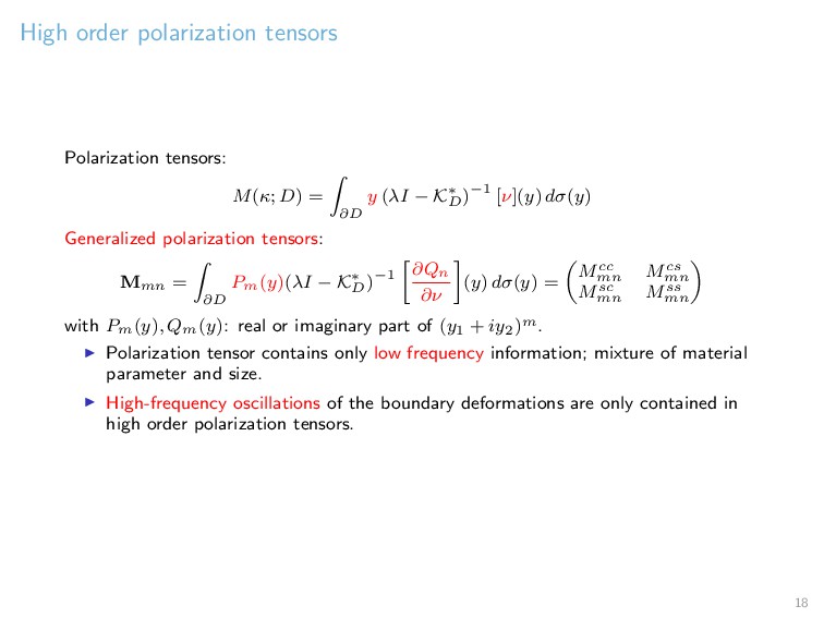
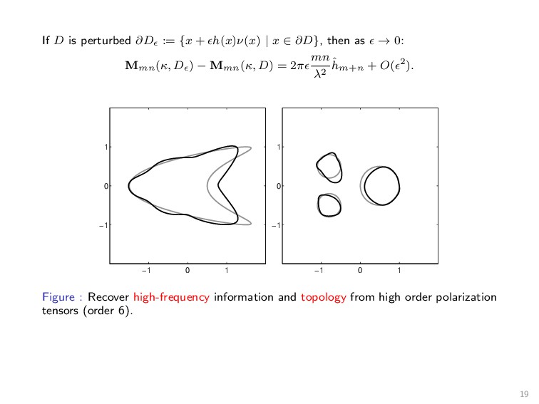
18. High order polarization tensors Polarization tensors: M(κ; D) = ∂D y (λI − K∗ D )−1 [ν](y) dσ(y) Generalized polarization tensors: Mmn = ∂D Pm(y)(λI − K∗ D )−1 ∂Qn ∂ν (y) dσ(y) = Mcc mn Mcs mn Msc mn Mss mn with Pm(y), Qm(y): real or imaginary part of (y1 + iy2)m. Polarization tensor contains only low frequency information; mixture of material parameter and size. High-frequency oscillations of the boundary deformations are only contained in high order polarization tensors. 18
19. If D is perturbed ∂D := {x + h(x)ν(x) | x ∈ ∂D}, then as → 0: Mmn(κ, D ) − Mmn(κ, D) = 2π mn λ2 ˆ hm+n + O( 2). −1 0 1 −1 0 1 −1 0 1 −1 0 1 Figure : Recover high-frequency information and topology from high order polarization tensors (order 6). 19
20. Multi-polar expansion6 Multistatic response matrix: Vsr := u(xr) − H(xr), with H(x) = Γ(x) + SΩ ∂u ∂ν + (x) − ξDΩ ∂u ∂ν + (x) Multi-polar expansion Vsr = K+1 m+n=1 SsmMmnR(s) nr L(M)sr +O(δK+2). Extraction of feature: M = arg min M L(M) − V L is exponentially ill-conditionned. Mmn decays exponentially with m + n. Maximum resolving order: K log σnoise log(R/δ) 6 Shape recognition and classification in electro-sensing, H.Ammari, T.Boulier, J.Garnier, H.Wang, To appear in PNAS 20
21. Transform invariant shape descriptors7 Scaling: Mmn(sD) = sm+nMmn(D) Rotation: Mmn(RθD) = ei(m+n)θMmn(D) Translation: Mmn(D + z) = m l=1 n k=1 Cz ml Mlk(D)Cz nk Registration point: for D = z + sRθB, M12(D) 2M11(D) u(D) = z + seiθ M12(B) 2M11(B) u(B) Construct transform invariant shape descriptors I so that I(D) = I(z + sRθD) for arbitrary scaling, rotation, and translation. 7 Target identification using dictionary matching of generalized polarization tensors, with H.Ammari, T.Boulier, J.Garnier, W.Jing, and H.Kang, in Foundations of Computational Mathematics, 2014 21
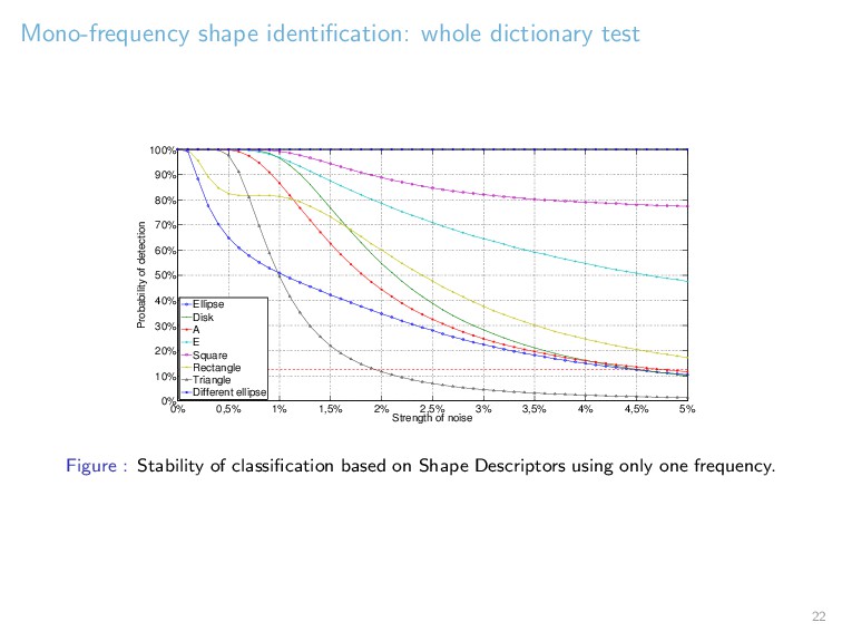
22. Mono-frequency shape identification: whole dictionary test 0% 0,5% 1% 1,5% 2% 2,5% 3% 3,5% 4% 4,5% 5% 0% 10% 20% 30% 40% 50% 60% 70% 80% 90% 100% Strength of noise Probability of detection Ellipse Disk A E Square Rectangle Triangle Different ellipse Figure : Stability of classification based on Shape Descriptors using only one frequency. 22
23. Shape identification: large dictionary Figure : Classification based on Shape Descriptors on a dictionary of 26 letters 23
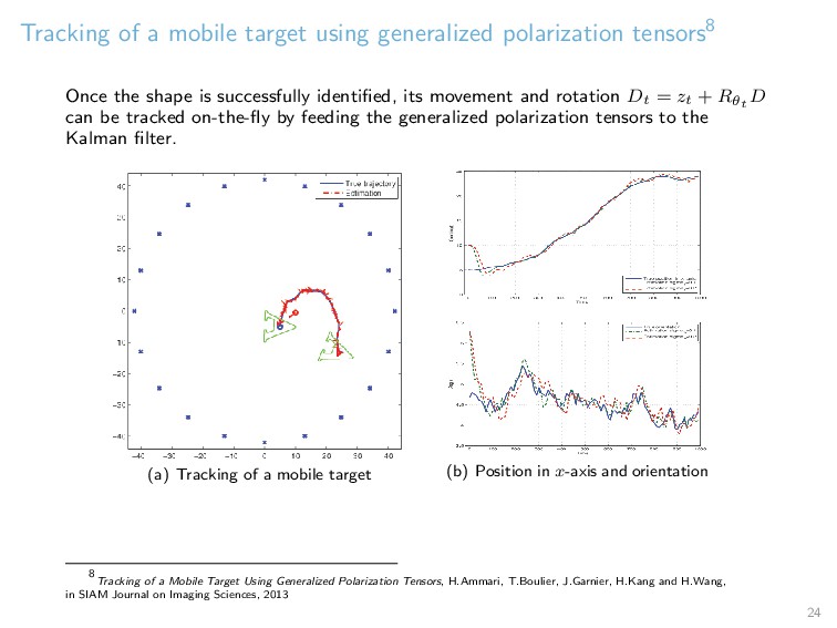
24. Tracking of a mobile target using generalized polarization tensors8 Once the shape is successfully identified, its movement and rotation Dt = zt + Rθt D can be tracked on-the-fly by feeding the generalized polarization tensors to the Kalman filter. (a) Tracking of a mobile target (b) Position in x-axis and orientation 8 Tracking of a Mobile Target Using Generalized Polarization Tensors, H.Ammari, T.Boulier, J.Garnier, H.Kang and H.Wang, in SIAM Journal on Imaging Sciences, 2013 24
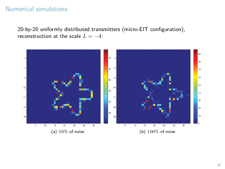
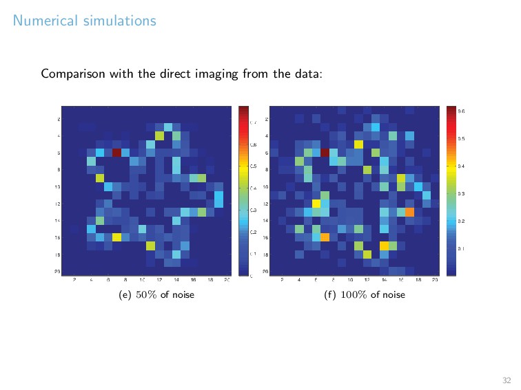
25. Near field measurement (micro-EIT) and stability (c) EIT (d) Micro-EIT (e) Stabilities More information can be reconstructed with near field measurement. How to choose the right basis for the representation and reconstruction of features? 25
26. From global to local features9 Bounded bilinear form T : H2(Rd) × H1(Rd) → R: T (f, g) := ∂D g(x)(λI − K∗ D )−1 ∂f ∂ν (x) ds(x) D = D if and only if their associated T are the same Representation of T ↔ features of D: Xmn = T (em, en) {em}m is a basis of Hs(Rd), s = 1, 2. – polynomial basis: generalized polarization tensors, global feature – wavelet basis: local feature Multistatic response matrix (EIT in free space): Vsr = ∂D Γr(x)(λI − K∗ D )−1 ∂Γs ∂ν (x) ds(x) Asymptotic expansion: Vsr = T (PK Γs, PK Γr) + Esr γs Xγr L(X)sr 9 Wavelet methods for shape perception in electro-sensing with H.Ammari, S.Mallat, and I.Waldspurger, submitted to Mathematics of Computation, 2013 26
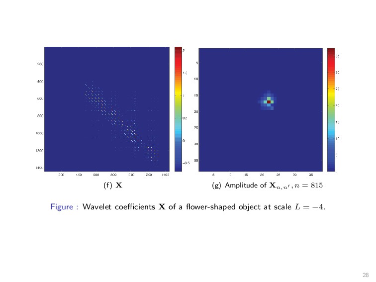
27. Properties of the wavelet coefficient matrix Daubechies scaling function of order 6: φ ∈ Cr 0 (R2), r ≥ 2. φL,n(x) = 2−Lφ(2−Lx − n), L ∈ Z, n ∈ Z2 Orthonormal basis of L2(R2), basis of Hs(R2), s = 1, 2. Xn,n = T (φL,n, φL,n ) = ∂D φL,n (x)(λI − K∗ D )−1 ∂φL,n ∂ν (x)ds(x). Very high dimension: ∼ 2−4L coefficients Very high sparsity: ∼ 22L (ratio of non-zeros) Localization of the boundary by the diagonal coefficients: |T (φL,n, φL,n )| = O(2−2L) for overlapped φL,n, φL,n , O(2−L) otherwise. 27
28. (f) X (g) Amplitude of Xn,n , n = 815 Figure : Wavelet coefficients X of a flower-shaped object at scale L = −4. 28
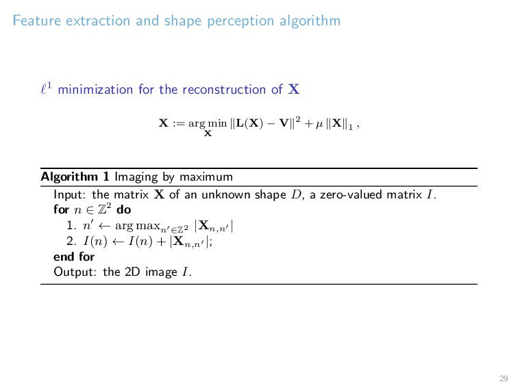
29. Feature extraction and shape perception algorithm 1 minimization for the reconstruction of X X := arg min X L(X) − V 2 + µ X 1 , Algorithm 1 Imaging by maximum Input: the matrix X of an unknown shape D, a zero-valued matrix I. for n ∈ Z2 do 1. n ← arg max n ∈Z2 |Xn,n | 2. I(n) ← I(n) + |Xn,n |; end for Output: the 2D image I. 29
30. Numerical simulations 20-by-20 uniformly distributed transmitters (micro-EIT configuration), reconstruction at the scale L = −4: (a) 50% of noise (b) 100% of noise 30
31. Numerical simulations 20-by-20 uniformly distributed transmitters (micro-EIT configuration), reconstruction at the scale L = −5: (c) 10% of noise (d) 50% of noise 31
32. Numerical simulations Comparison with the direct imaging from the data: (e) 50% of noise (f) 100% of noise 32
33. Echolocation 33
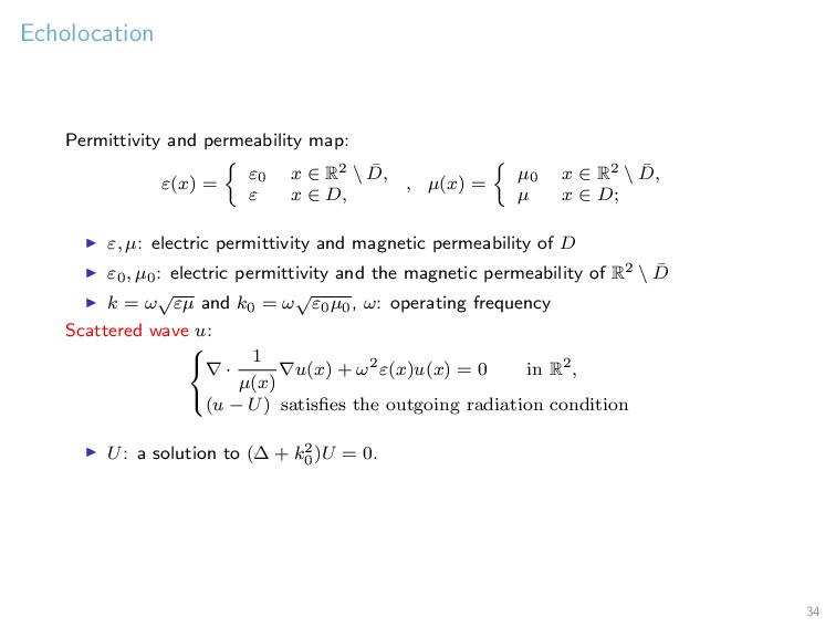
34. Echolocation Permittivity and permeability map: ε(x) = ε0 x ∈ R2 \ ¯ D, ε x ∈ D, , µ(x) = µ0 x ∈ R2 \ ¯ D, µ x ∈ D; ε, µ: electric permittivity and magnetic permeability of D ε0, µ0: electric permittivity and the magnetic permeability of R2 \ ¯ D k = ω √ εµ and k0 = ω √ ε0µ0, ω: operating frequency Scattered wave u:    ∇ · 1 µ(x) ∇u(x) + ω2ε(x)u(x) = 0 in R2, (u − U) satisfies the outgoing radiation condition U: a solution to (∆ + k2 0 )U = 0. 34
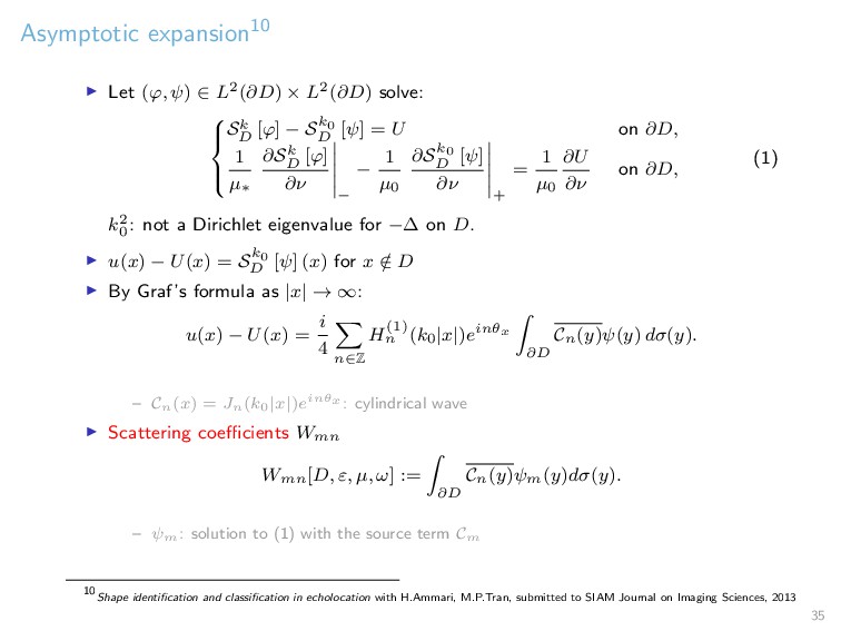
35. Asymptotic expansion10 Let (ϕ, ψ) ∈ L2(∂D) × L2(∂D) solve:      Sk D [ϕ] − Sk0 D [ψ] = U on ∂D, 1 µ∗ ∂Sk D [ϕ] ∂ν − − 1 µ0 ∂Sk0 D [ψ] ∂ν + = 1 µ0 ∂U ∂ν on ∂D, (1) k2 0 : not a Dirichlet eigenvalue for −∆ on D. u(x) − U(x) = Sk0 D [ψ] (x) for x / ∈ D By Graf’s formula as |x| → ∞: u(x) − U(x) = i 4 n∈Z H(1) n (k0|x|)einθx ∂D Cn(y)ψ(y) dσ(y). – Cn(x) = Jn(k0|x|)einθx : cylindrical wave Scattering coefficients Wmn Wmn[D, ε, µ, ω] := ∂D Cn(y)ψm(y)dσ(y). – ψm: solution to (1) with the source term Cm 10 Shape identification and classification in echolocation with H.Ammari, M.P.Tran, submitted to SIAM Journal on Imaging Sciences, 2013 35
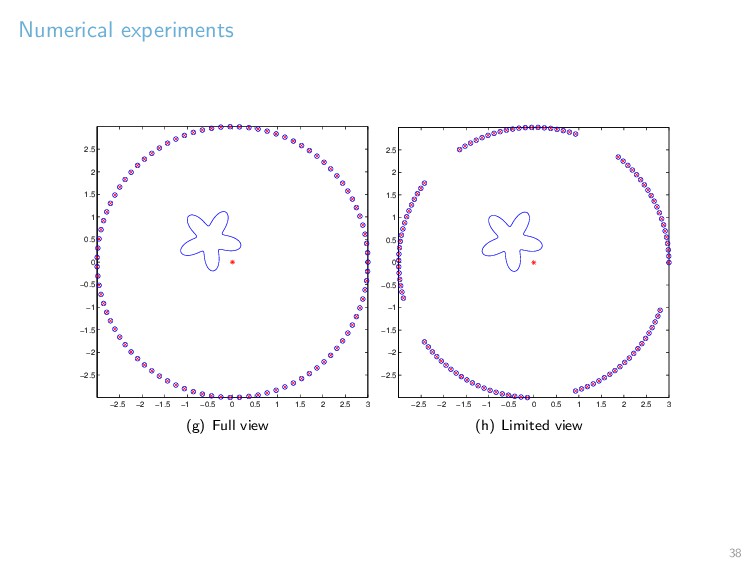
36. Feature extraction Location algorithm yields z, the position of D Use plane wave source Us(x) = eik0ξs·x with equally distributed receptors xr Multistatic response matrix Vsr = us(xr) − Us(xr) Linear system: Vsr = m,n∈Z AsmWmn[D − z](B∗)nr = L(W), A, B depend only on the sources and receptors. Extract W by solving a least-squares method W = arg min W L(W) − V L is ill-conditionned, W decays rapidely: |Wmn| C0 |m|+|n| |m||m||n||n| for all m, n ∈ Z. Maximum resolving order K: KK+1/2 SNR 36
37. Shape descriptors Connection with the far field pattern: A∞ D (ξ; ω) = m,n∈Z Wmn[D, ε, µ, ω]eim( π 2 −ξ1)e−in( π 2 −ξ2). (2) For D = z + sRθB, then A∞ D (ξ; ω) = φz(ξ) A∞ B (ξθ; sω) with ξθ := ξ − (θ, θ) . with φz(ξ) := eik0|z| cos(ξ1−θz)e−ik0|z| cos(ξ2−θz). Shape descriptor: SD(v; ω) := [0,2π]2 |A∞ D (ξ; ω)A∞ D (ξ − v; ω)| dξ Invariant to translation and rotation: SD(v; ω) = SB(v; sω). Scaling parameter is estimated using multi-frequency s = arg min s∈[smin,smax]    ωmax ωmin [0,2π]2 [SD(v; ω) − SB(v; sω)] dv 2 dω    . Matching in a multi-frequency dictionary of shape descriptors by estimating the scaling parameter 37
38. Numerical experiments −2.5 −2 −1.5 −1 −0.5 0 0.5 1 1.5 2 2.5 3 −2.5 −2 −1.5 −1 −0.5 0 0.5 1 1.5 2 2.5 (g) Full view −2.5 −2 −1.5 −1 −0.5 0 0.5 1 1.5 2 2.5 3 −2.5 −2 −1.5 −1 −0.5 0 0.5 1 1.5 2 2.5 (h) Limited view 38
39. Numerical experiments Far field pattern A∞ D (ξ; 2π) of a flower-shaped object: 50 100 150 200 250 300 350 400 450 500 50 100 150 200 250 300 350 400 450 500 4 6 8 10 12 14 16 18 (i) Full view 50 100 150 200 250 300 350 400 450 500 50 100 150 200 250 300 350 400 450 500 2 4 6 8 10 12 14 16 18 (j) Limited view 39
40. Numerical experiments Ellipse Flower A Square E Rectangle Circle Triangle 0 100 200 300 400 500 600 700 (k) Full view Ellipse Flower A Square E Rectangle Circle Triangle 0 1 2 3 4 5 6 (l) Limited view 40
41. Conclusion Physics-based identification approach for solving nonlinear inverse problems Representation of geometric information: global (or local) features for far-field (or near-field or internal) measurements. Feature extraction from measurements and construction of invariants. Classfication and identification in a dictionary. Potential applications in engineering and other type of physics. Thank you! 41