Biohub - Cell Tracking During Development - 3rd Place Solution

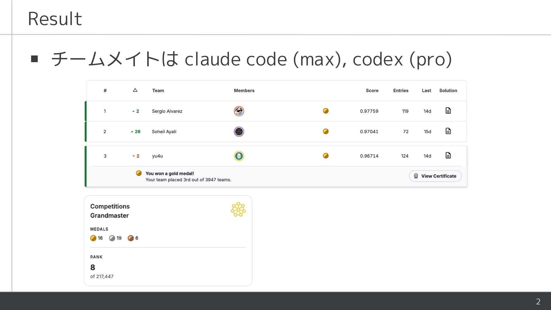
Kaggleコンペ「Biohub - Cell Tracking During Development」で3位（全3,947チーム）を獲得したソリューションの解説資料です。

本コンペは、ゼブラフィッシュ胚の3次元タイムラプス顕微鏡画像から細胞を検出・追跡し、細胞分裂を含む系譜グラフを構築するタスクです。正解データが全細胞の約2.8%しか存在しない疎なアノテーションや、学習・テスト間の胚の違いなどが課題となりました。

ソリューションでは、2.5D/3Dモデルによる細胞検出、自己教師あり学習によるDense Flow推定、Transformerによる細胞マッチング、細胞分裂の検出を組み合わせた多段パイプラインを構築。さらに、TP・FPの期待値を用いて評価指標を近似し、LP/MILPによるグラフ全体の最適化を行いました。

各モデルのアーキテクチャや学習方法に加え、確率較正、後処理、CV設計、アブレーション結果、うまくいかなかったアプローチなどを紹介しています。

Transcript

1. Biohub - Cell Tracking During Development rd 3 Place Solution 内田 祐介 GOドライブ株式会社 AI Community
2. Result ▪ チームメイトは claude code (max), codex (pro) 2
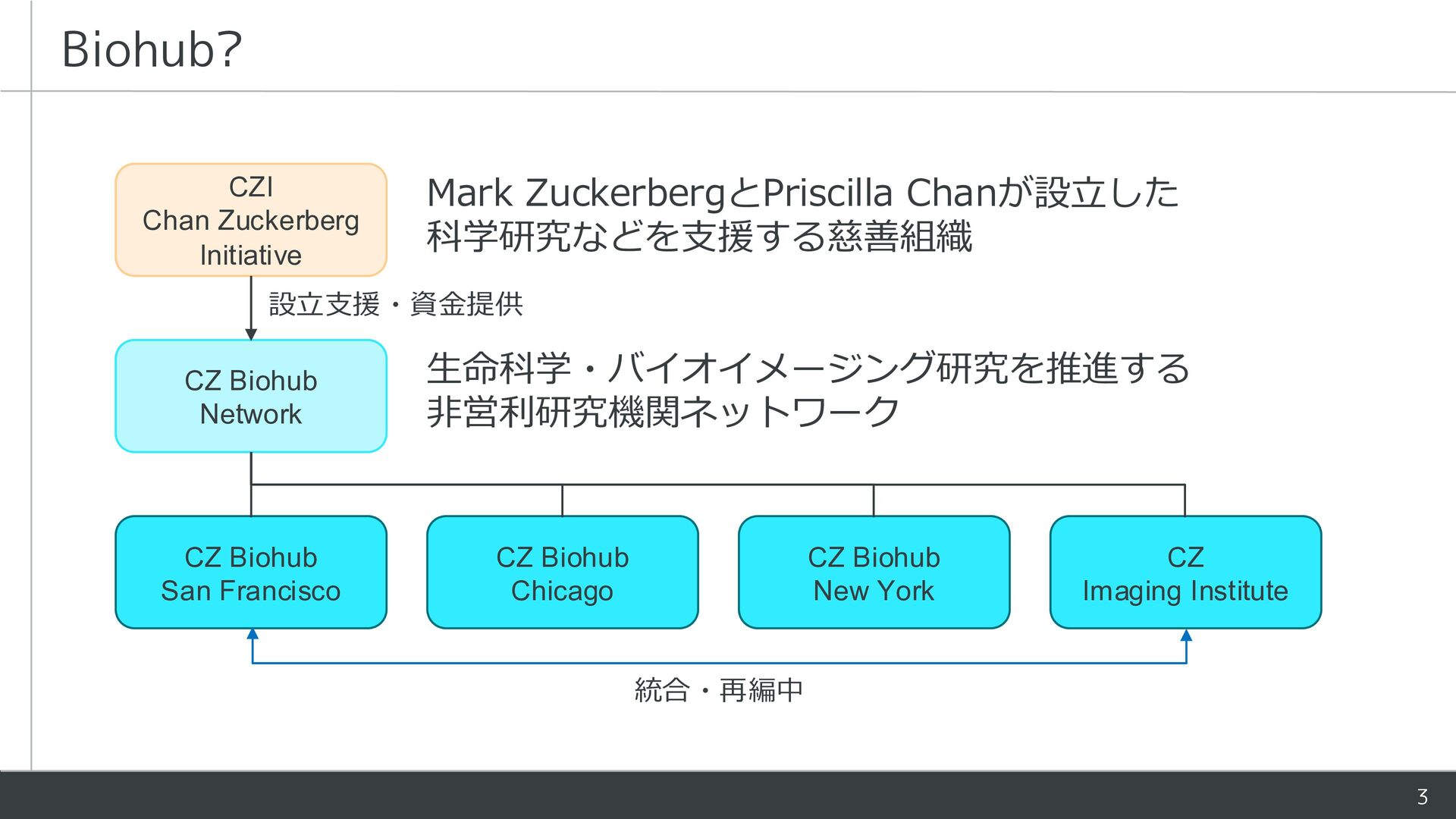
3. Biohub? CZI Chan Zuckerberg Initiative Mark ZuckerbergとPriscilla Chanが設立した 科学研究などを支援する慈善組織 設立支援・資金提供 CZ Biohub Network CZ Biohub San Francisco 生命科学・バイオイメージング研究を推進する 非営利研究機関ネットワーク CZ Biohub Chicago CZ Biohub New York CZ Imaging Institute 統合・再編中 3
4. CZII? 4
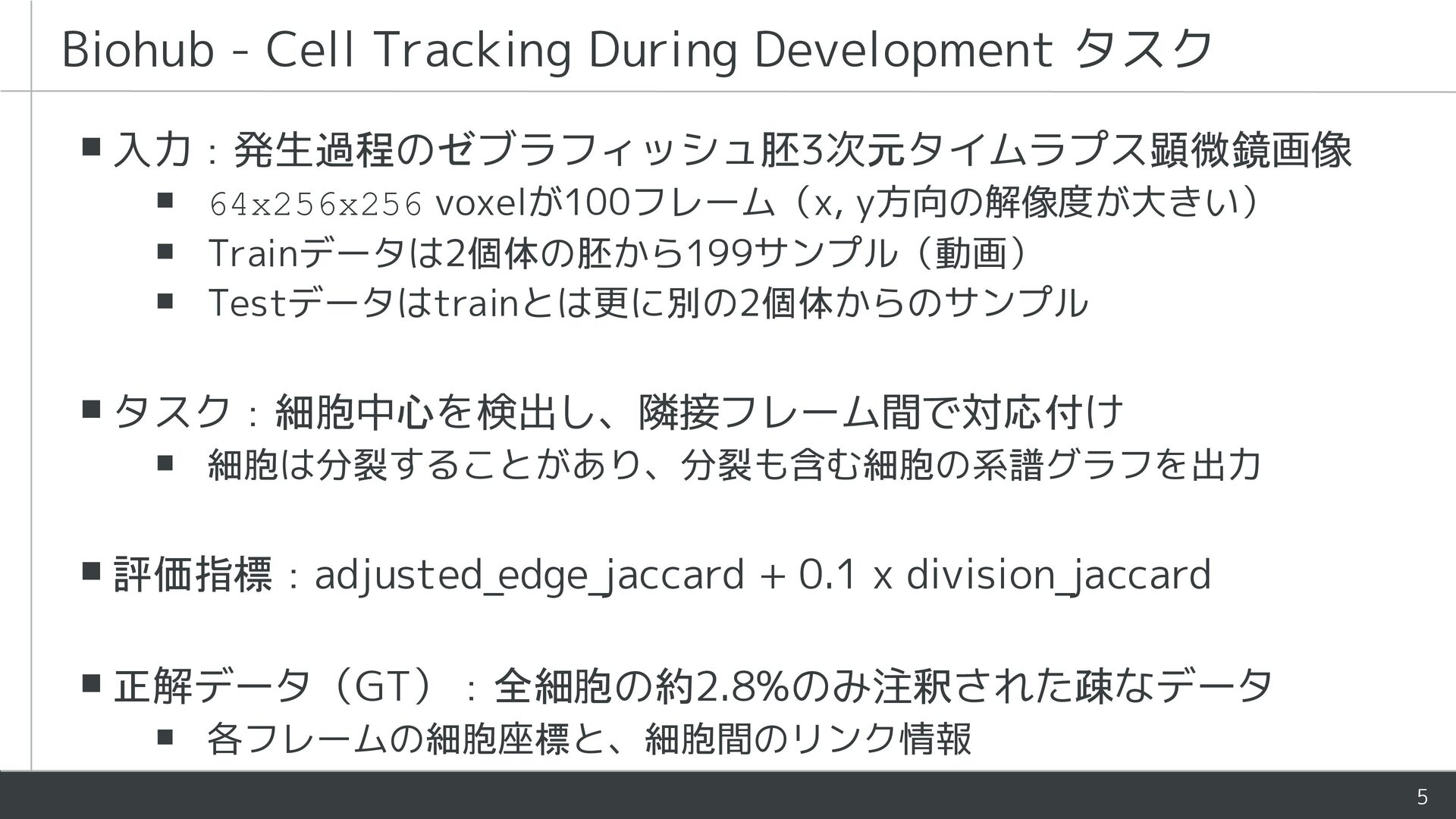
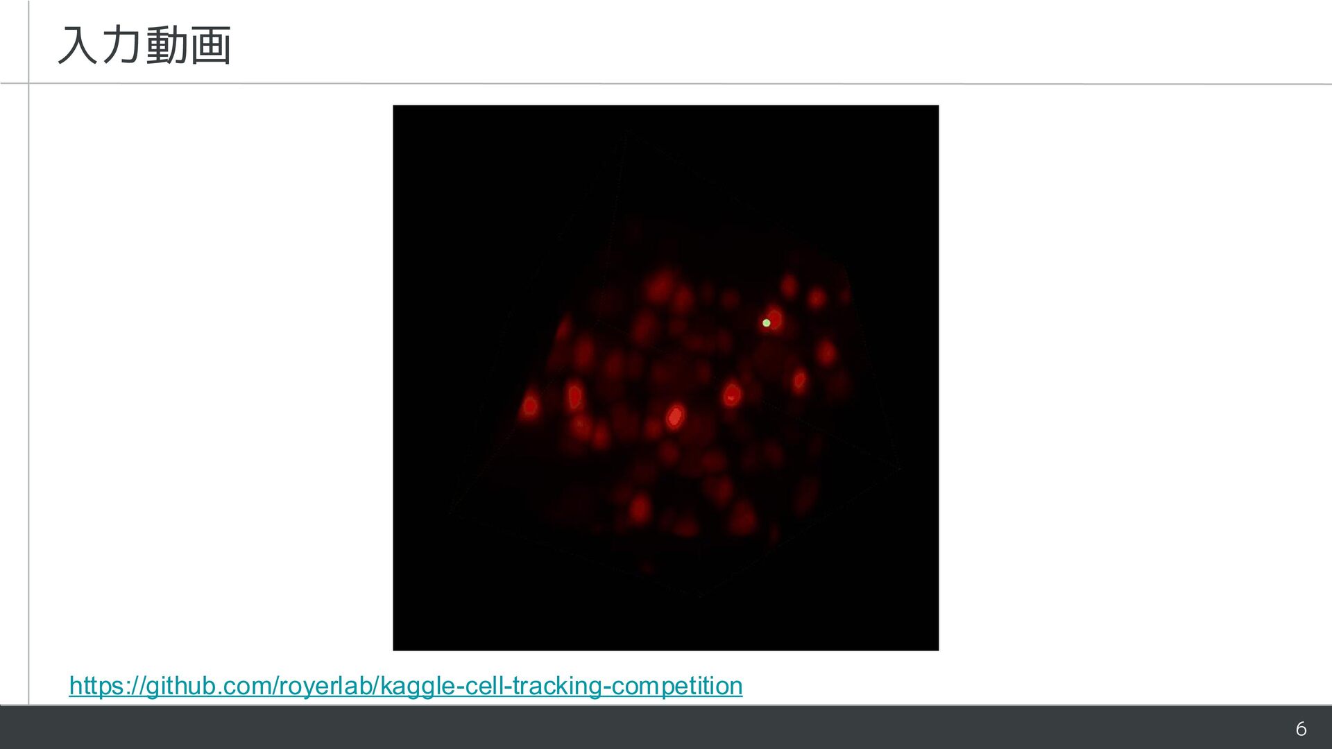
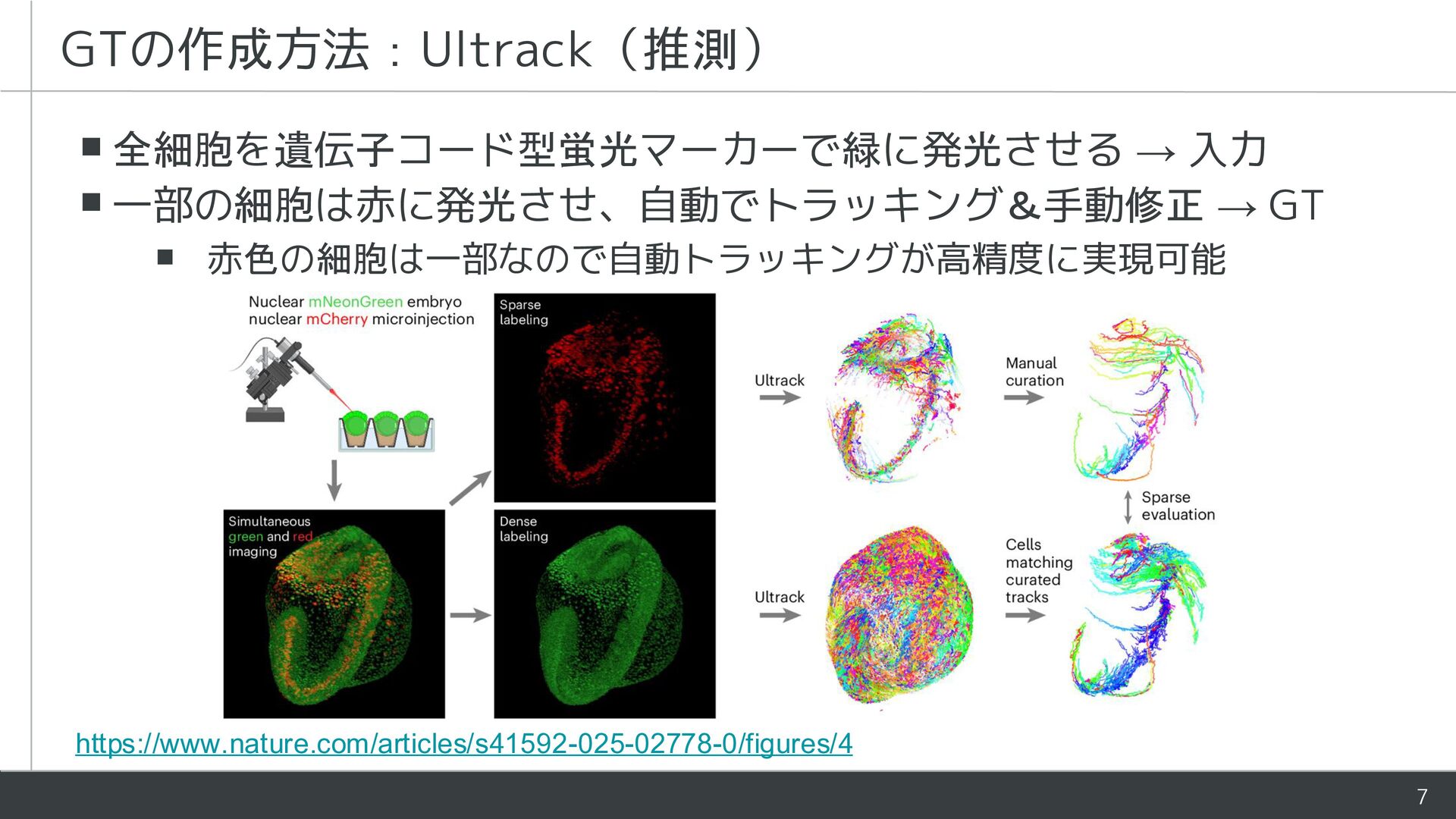
5. Biohub - Cell Tracking During Development タスク ▪ 入力：発生過程のゼブラフィッシュ胚3次元タイムラプス顕微鏡画像 ▪ 64x256x256 voxelが100フレーム（x, y方向の解像度が大きい） ▪ Trainデータは2個体の胚から199サンプル（動画） ▪ Testデータはtrainとは更に別の2個体からのサンプル ▪ タスク：細胞中心を検出し、隣接フレーム間で対応付け ▪ 細胞は分裂することがあり、分裂も含む細胞の系譜グラフを出力 ▪ 評価指標：adjusted_edge_jaccard + 0.1 x division_jaccard ▪ 正解データ（GT）：全細胞の約2.8%のみ注釈された疎なデータ ▪ 各フレームの細胞座標と、細胞間のリンク情報 5
6. 入力動画 https://github.com/royerlab/kaggle-cell-tracking-competition 6
7. GTの作成方法：Ultrack（推測） ▪ 全細胞を遺伝子コード型蛍光マーカーで緑に発光させる → 入力 ▪ 一部の細胞は赤に発光させ、自動でトラッキング＆手動修正 → GT ▪ 赤色の細胞は一部なので自動トラッキングが高精度に実現可能 https://www.nature.com/articles/s41592-025-02778-0/figures/4 7
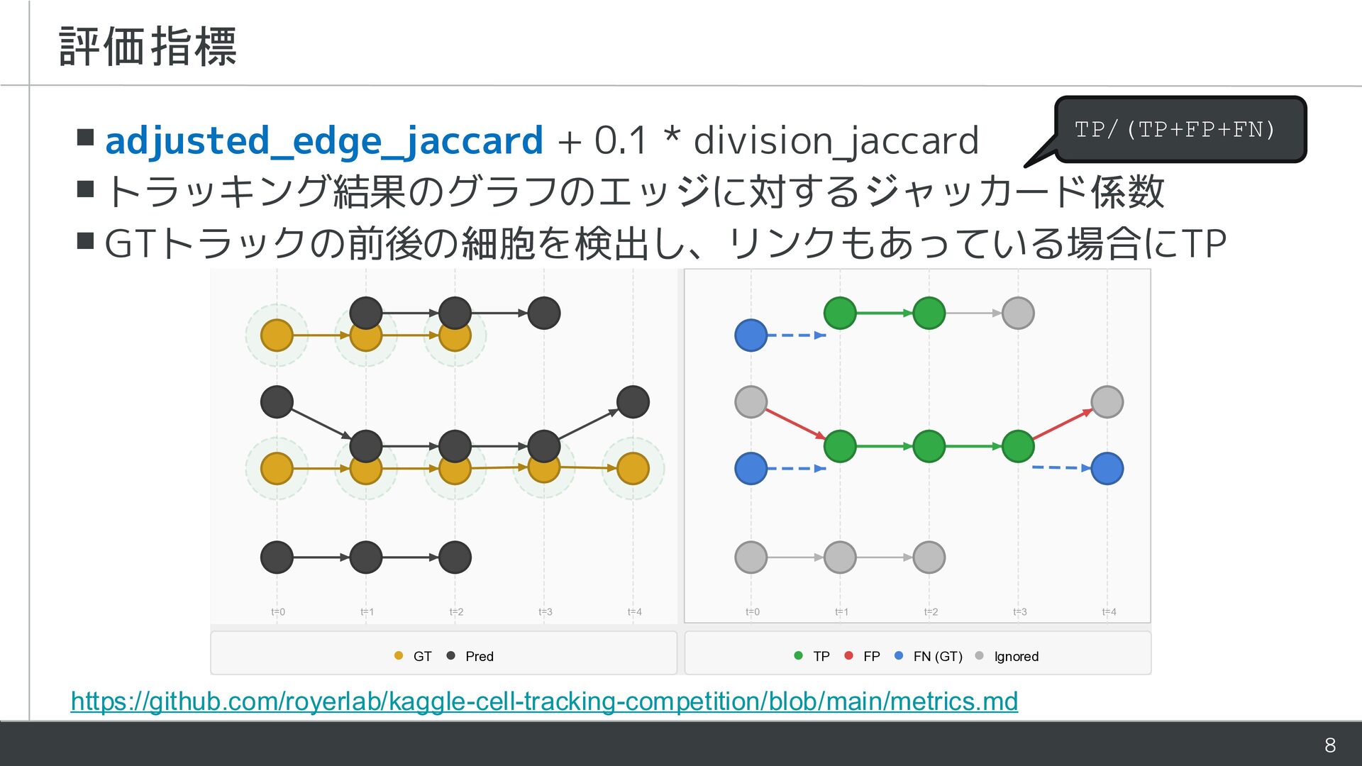
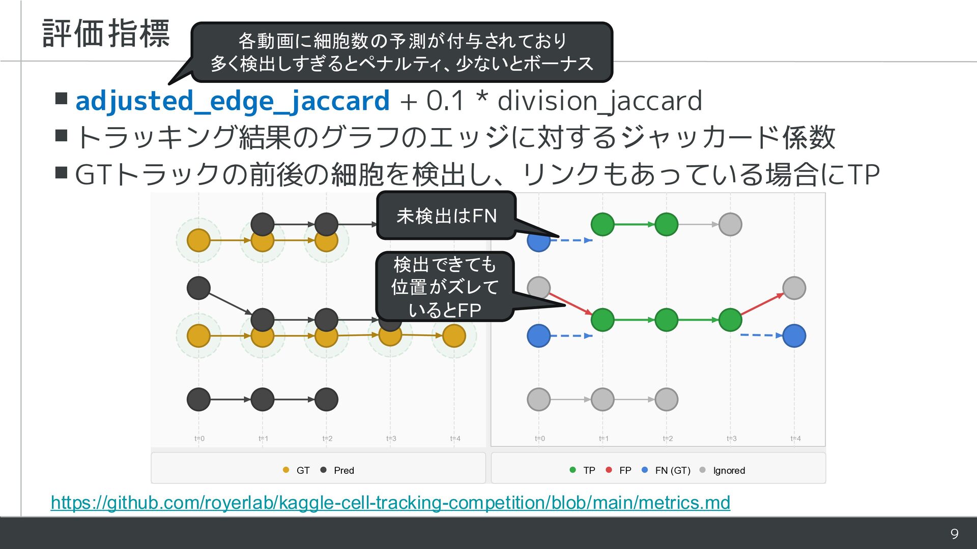
8. 評価指標 ▪ adjusted_edge_jaccard + 0.1 * division_jaccard ▪ トラッキング結果のグラフのエッジに対するジャッカード係数 ▪ GTトラックの前後の細胞を検出し、リンクもあっている場合にTP TP/(TP+FP+FN) https://github.com/royerlab/kaggle-cell-tracking-competition/blob/main/metrics.md 8
9. 評価指標 各動画に細胞数の予測が付与されており 多く検出しすぎるとペナルティ、少ないとボーナス ▪ adjusted_edge_jaccard + 0.1 * division_jaccard ▪ トラッキング結果のグラフのエッジに対するジャッカード係数 ▪ GTトラックの前後の細胞を検出し、リンクもあっている場合にTP 未検出はFN 検出できても 位置がズレて いるとFP https://github.com/royerlab/kaggle-cell-tracking-competition/blob/main/metrics.md 9
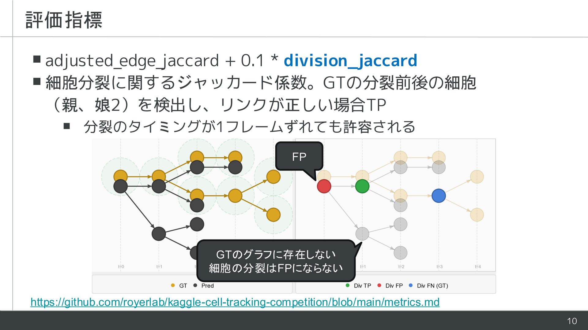
10. 評価指標 ▪ adjusted_edge_jaccard + 0.1 * division_jaccard ▪ 細胞分裂に関するジャッカード係数。GTの分裂前後の細胞 （親、娘2）を検出し、リンクが正しい場合TP ▪ 分裂のタイミングが1フレームずれても許容される FP GTのグラフに存在しない 細胞の分裂はFPにならない https://github.com/royerlab/kaggle-cell-tracking-competition/blob/main/metrics.md 10
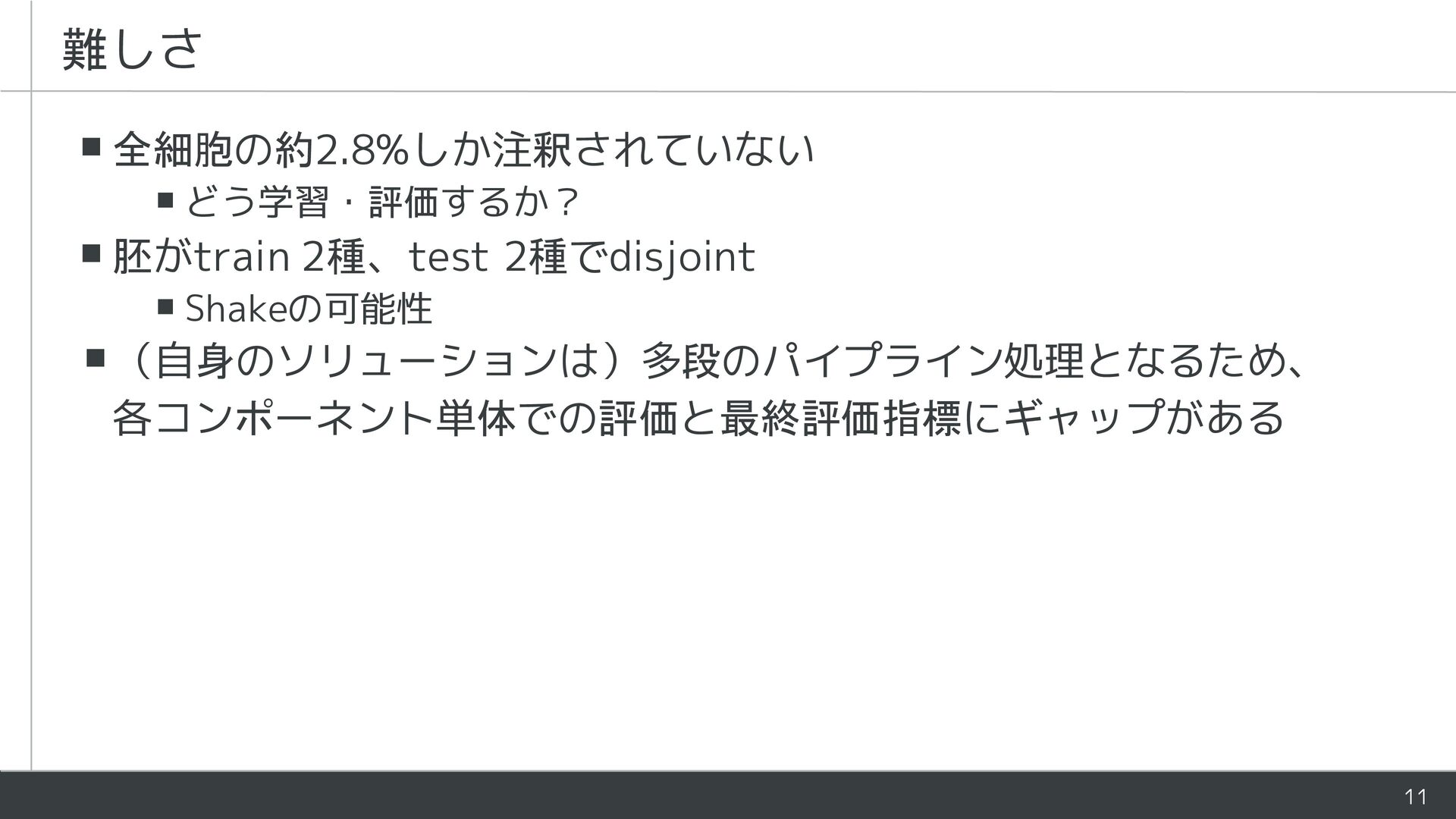
11. 難しさ ▪ 全細胞の約2.8%しか注釈されていない ▪ どう学習・評価するか？ ▪ 胚がtrain 2種、test 2種でdisjoint ▪ Shakeの可能性 ▪（自身のソリューションは）多段のパイプライン処理となるため、 各コンポーネント単体での評価と最終評価指標にギャップがある 11
12. Probe結果 ▪ Embryo単位でpublic testとprivate testが分かれている！ ▪ Publicとprivateで細胞密度が結構違う ▪ 両方のembryoが改善するアプローチのみ採用 → CVとLBが相関 12
13. ベースライン ▪ 主催者がベースラインパイプラインを提供 ▪https://github.com/royerlab/kaggle-cell-trackingcompetition ▪ TemporalUNet3D + SimpleNodeTransformer ▪細胞検出と細胞間のリンク予測を同時に解くモデル 13
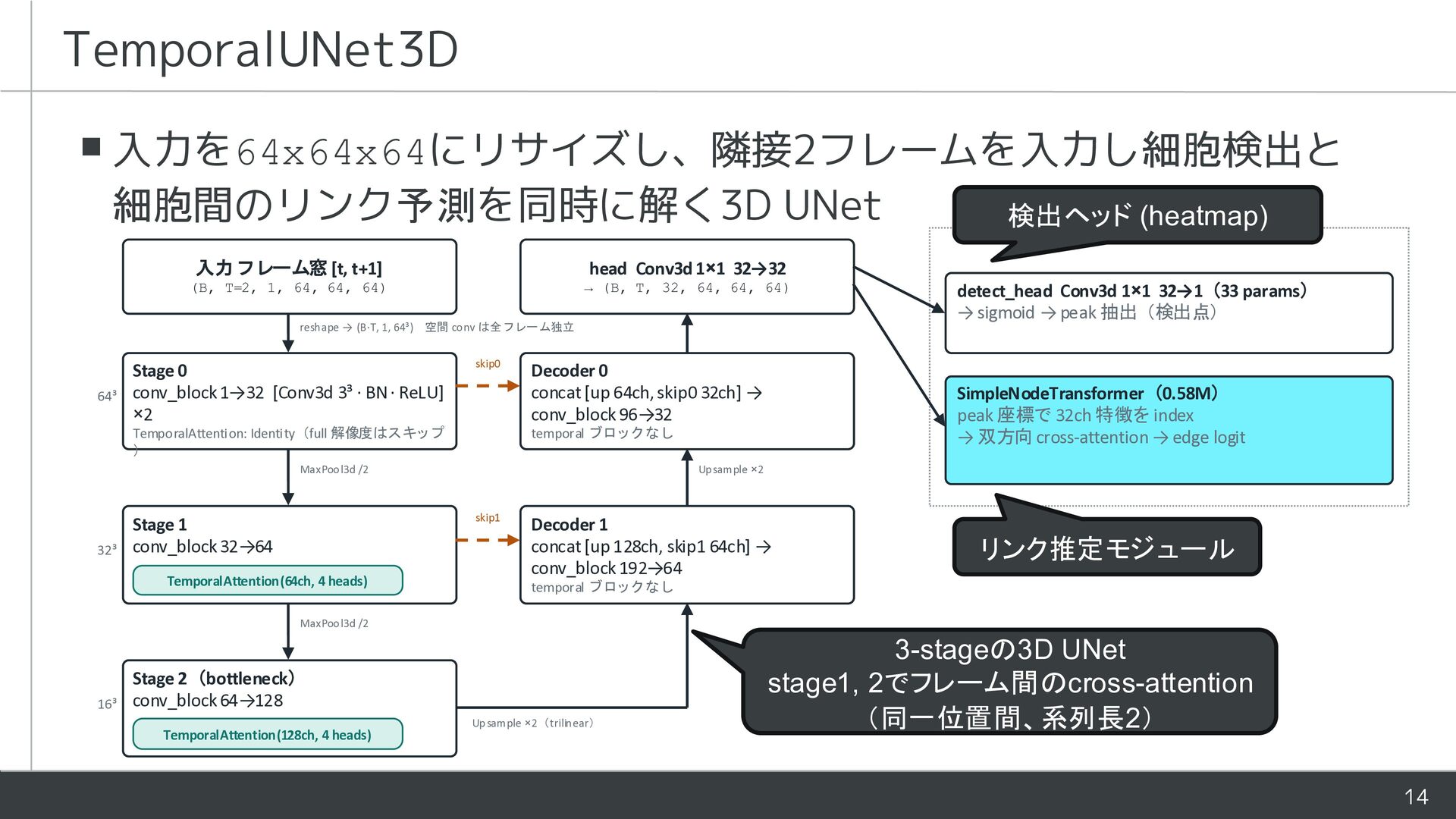
14. TemporalUNet3D ▪ 入力を64x64x64にリサイズし、隣接2フレームを入力し細胞検出と 細胞間のリンク予測を同時に解く3D UNet 入力 フレーム窓 [t, t+1] head Conv3d 1×1 32→32 (B, T=2, 1, 64, 64, 64) → (B, T, 32, 64, 64, 64) resh ape → (B·T, 1, 64³) 64³ 空間 co nv は全 フレー ム独立 Stage 0 conv_block 1→32 [Conv3d 3³ · BN · ReLU] ×2 skip0 TemporalAttention: Identity（full 解像度はスキップ ） Decoder 0 concat [up 64ch, skip0 32ch] → conv_block 96→32 32³ Upsample ×2 skip1 TemporalAttention(64ch, 4 heads) detect_head Conv3d 1×1 32→1（33 params） → sigmoid → peak 抽出（検出点） SimpleNodeTransformer（0.58M） peak 座標で 32ch 特徴を index → 双方向 cross-attention → edge logit temporal ブロックなし MaxPoo l3d /2 Stage 1 conv_block 32→64 検出ヘッド (heatmap) Decoder 1 concat [up 128ch, skip1 64ch] → conv_block 192→64 リンク推定モジュール temporal ブロックなし MaxPool3d /2 16³ Stage 2（bottleneck） conv_block 64→128 TemporalAttention(128ch, 4 heads) Upsample ×2（trilinear） 3-stageの3D UNet stage1, 2でフレーム間のcross-attention （同一位置間、系列長2） 14
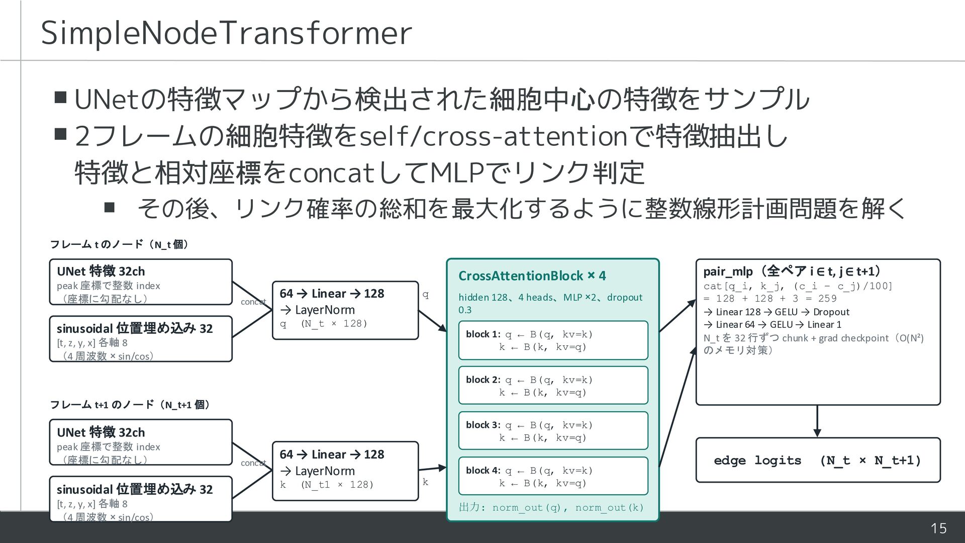
15. SimpleNodeTransformer ▪ UNetの特徴マップから検出された細胞中心の特徴をサンプル ▪ 2フレームの細胞特徴をself/cross-attentionで特徴抽出し 特徴と相対座標をconcatしてMLPでリンク判定 ▪ その後、リンク確率の総和を最大化するように整数線形計画問題を解く フレーム t のノード（N_t 個） UNet 特徴 32ch peak 座標で整数 index （座標に勾配なし） CrossAttentionBlock × 4 concat 64 → Linear → 128 → LayerNorm q sinusoidal 位置埋め込み 32 q (N_t × 128) hidden 128、4 heads、MLP ×2、dropout 0.3 block 1: q ← B(q, kv=k) k ← B(k, kv=q) [t, z, y, x] 各軸 8 （4 周波数 × sin/cos） pair_mlp（全ペア i ∈ t, j ∈ t+1） cat[q_i, k_j, (c_i − c_j)/100] = 128 + 128 + 3 = 259 → Linear 128 → GELU → Dropout → Linear 64 → GELU → Linear 1 N_t を 32 行ずつ chunk + grad checkpoint（O(N²) のメモリ対策） block 2: q ← B(q, kv=k) k ← B(k, kv=q) フレーム t+1 のノード（N_t+1 個） block 3: q ← B(q, kv=k) k ← B(k, kv=q) UNet 特徴 32ch peak 座標で整数 index （座標に勾配なし） sinusoidal 位置埋め込み 32 [t, z, y, x] 各軸 8 （4 周波数 × sin/cos） concat 64 → Linear → 128 → LayerNorm k (N_t1 × 128) k block 4: q ← B(q, kv=k) k ← B(k, kv=q) edge logits (N_t × N_t+1) 出力: norm_out(q), norm_out(k) 15
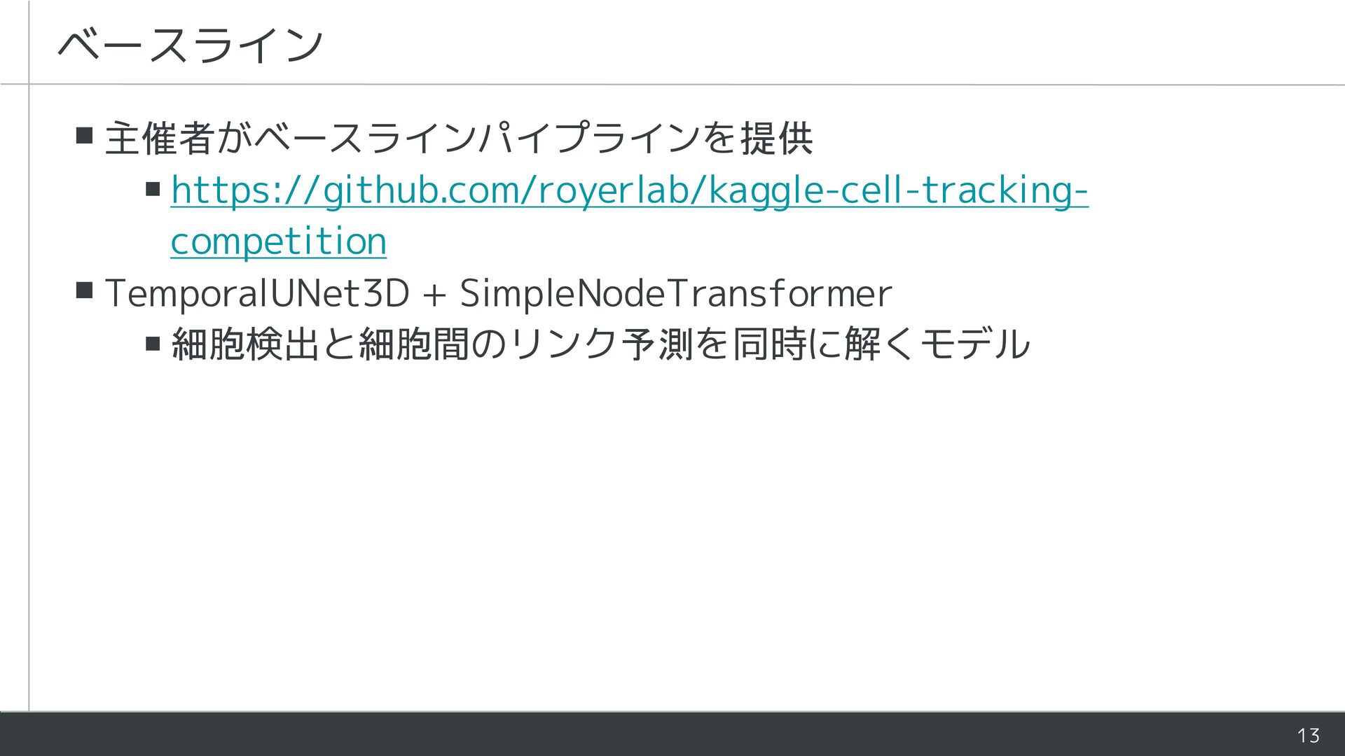
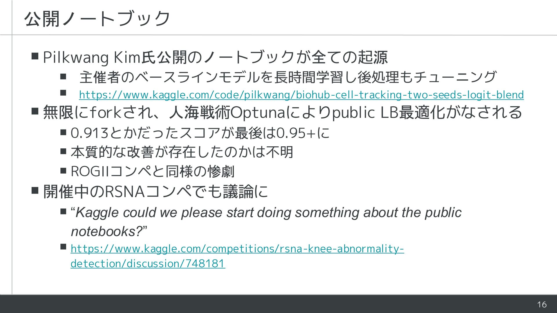
16. 公開ノートブック ▪ Pilkwang Kim氏公開のノートブックが全ての起源 ▪ 主催者のベースラインモデルを長時間学習し後処理もチューニング ▪ https://www.kaggle.com/code/pilkwang/biohub-cell-tracking-two-seeds-logit-blend ▪ 無限にforkされ、人海戦術Optunaによりpublic LB最適化がなされる ▪ 0.913とかだったスコアが最後は0.95+に ▪ 本質的な改善が存在したのかは不明 ▪ ROGIIコンペと同様の惨劇 ▪ 開催中のRSNAコンペでも議論に ▪ “Kaggle could we please start doing something about the public notebooks?” ▪ https://www.kaggle.com/competitions/rsna-knee-abnormalitydetection/discussion/748181 16
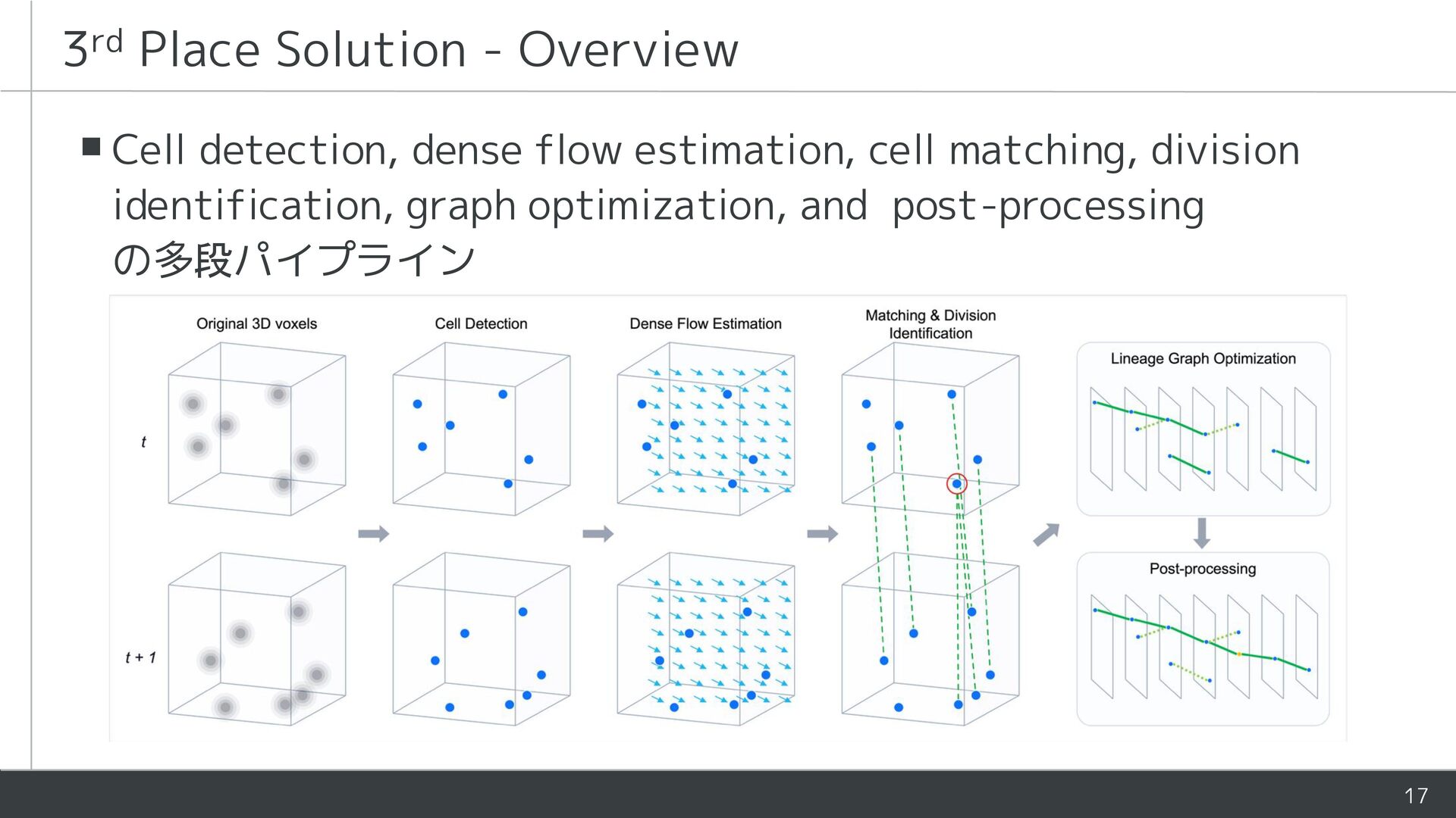
17. rd 3 Place Solution - Overview ▪ Cell detection, dense flow estimation, cell matching, division identification, graph optimization, and post-processing の多段パイプライン 17
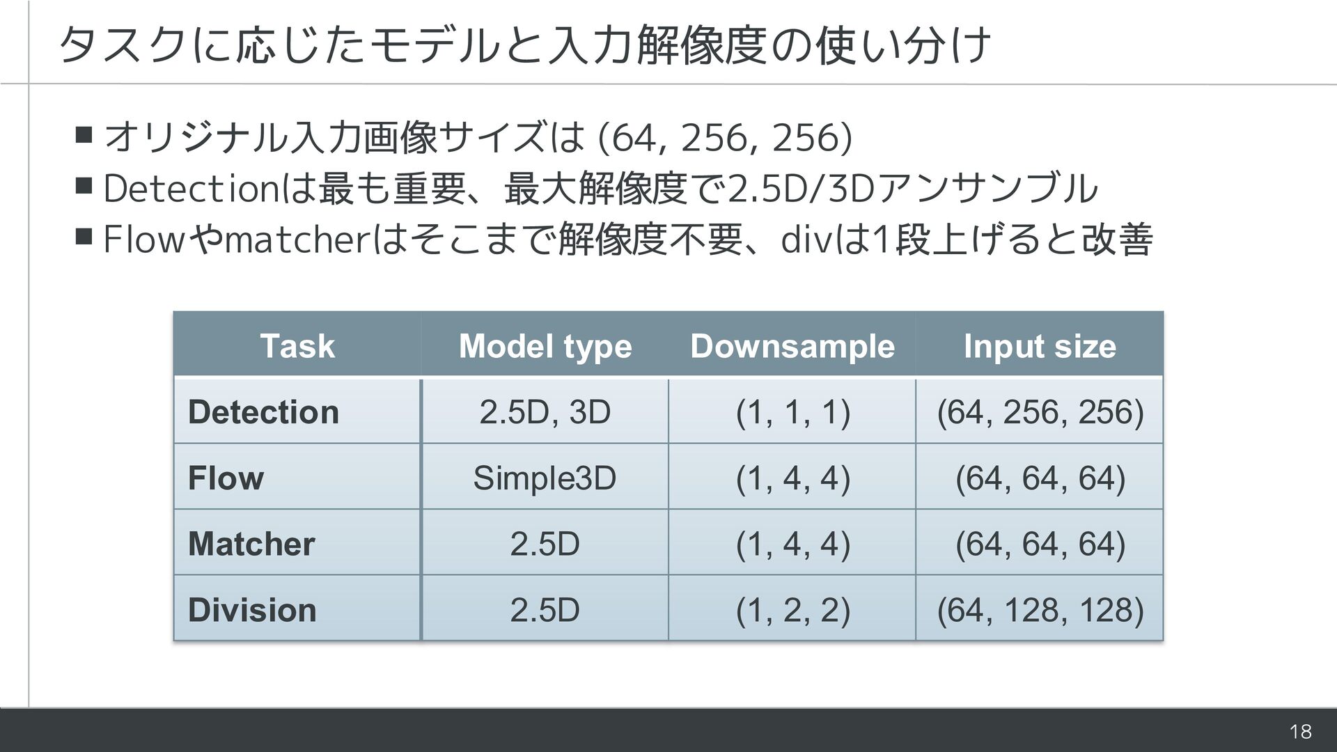
18. タスクに応じたモデルと入力解像度の使い分け ▪ オリジナル入力画像サイズは (64, 256, 256) ▪ Detectionは最も重要、最大解像度で2.5D/3Dアンサンブル ▪ Flowやmatcherはそこまで解像度不要、divは1段上げると改善 Task Model type Downsample Input size Detection 2.5D, 3D (1, 1, 1) (64, 256, 256) Flow Simple3D (1, 4, 4) (64, 64, 64) Matcher 2.5D (1, 4, 4) (64, 64, 64) Division 2.5D (1, 2, 2) (64, 128, 128) 18
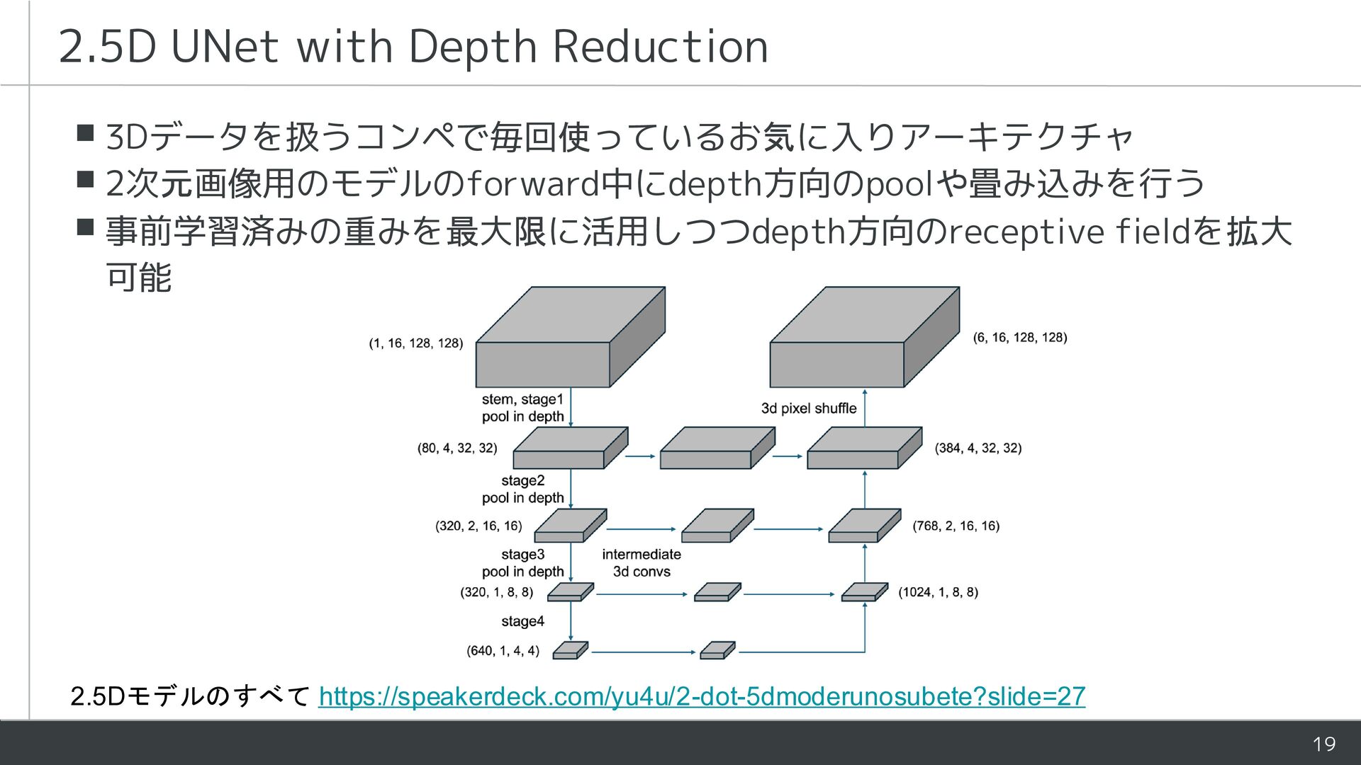
19. 2.5D UNet with Depth Reduction ▪ 3Dデータを扱うコンペで毎回使っているお気に入りアーキテクチャ ▪ 2次元画像用のモデルのforward中にdepth方向のpoolや畳み込みを行う ▪ 事前学習済みの重みを最大限に活用しつつdepth方向のreceptive fieldを拡大 可能 2.5Dモデルのすべて https://speakerdeck.com/yu4u/2-dot-5dmoderunosubete?slide=27 19
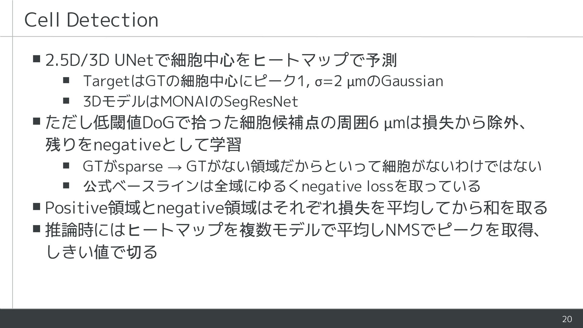
20. Cell Detection ▪ 2.5D/3D UNetで細胞中心をヒートマップで予測 ▪ TargetはGTの細胞中心にピーク1, σ=2 µmのGaussian ▪ 3DモデルはMONAIのSegResNet ▪ ただし低閾値DoGで拾った細胞候補点の周囲6 µmは損失から除外、 残りをnegativeとして学習 ▪ GTがsparse → GTがない領域だからといって細胞がないわけではない ▪ 公式ベースラインは全域にゆるくnegative lossを取っている ▪ Positive領域とnegative領域はそれぞれ損失を平均してから和を取る ▪ 推論時にはヒートマップを複数モデルで平均しNMSでピークを取得、 しきい値で切る 20
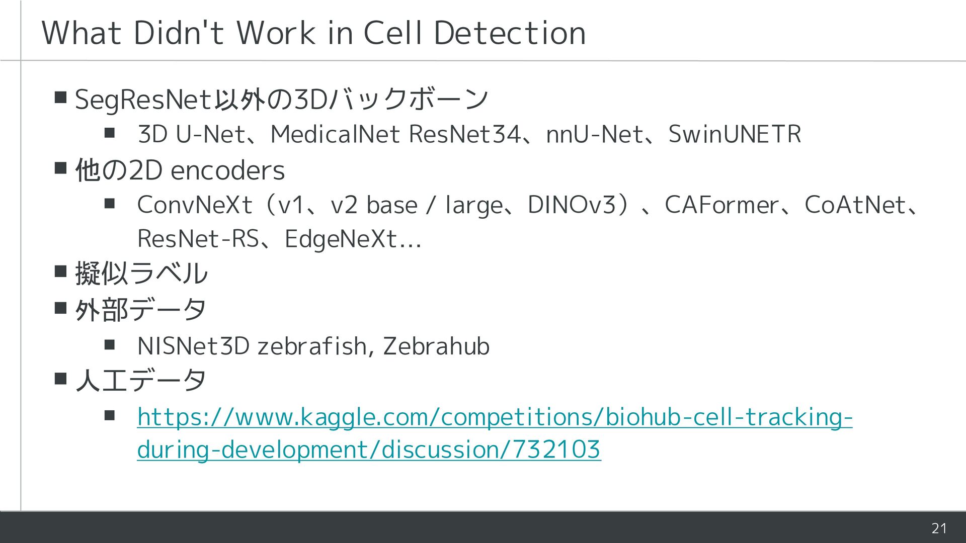
21. What Didn't Work in Cell Detection ▪ SegResNet以外の3Dバックボーン ▪ 3D U-Net、MedicalNet ResNet34、nnU-Net、SwinUNETR ▪ 他の2D encoders ▪ ConvNeXt（v1、v2 base / large、DINOv3）、CAFormer、CoAtNet、 ResNet-RS、EdgeNeXt… ▪ 擬似ラベル ▪ 外部データ ▪ NISNet3D zebrafish, Zebrahub ▪ 人工データ ▪ https://www.kaggle.com/competitions/biohub-cell-trackingduring-development/discussion/732103 21
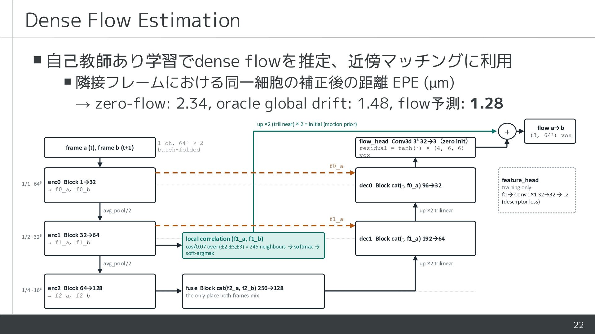
22. Dense Flow Estimation ▪ 自己教師あり学習でdense flowを推定、近傍マッチングに利用 ▪ 隣接フレームにおける同一細胞の補正後の距離 EPE (µm) → zero-flow: 2.34, oracle global drift: 1.48, flow予測: 1.28 up ×2 (trilinear) × 2 = initial (motion prior) frame a (t), frame b (t+1) + flow a→b (3, 64³) vox flow_head Conv3d 3³ 32→3（zero init） 1 ch, 64³ × 2 batch-folded residual = tanh(·) × (4, 6, 6) vox f0_a 1/1 · 64³ enc0 Block 1→32 dec0 Block cat(·, f0_a) 96→32 → f0_a, f0_b feature_head training only f0 → Conv 1×1 32→32 → L2 (descriptor loss) up ×2 trilinear avg_pool /2 f1_a 1/2 · 32³ enc1 Block 32→64 local correlation (f1_a, f1_b) → f1_a, f1_b cos/0.07 over (±2,±3,±3) = 245 neighbours → softmax → soft-argmax up ×2 trilinear avg_pool /2 1/4 · 16³ dec1 Block cat(·, f1_a) 192→64 enc2 Block 64→128 fuse Block cat(f2_a, f2_b) 256→128 → f2_a, f2_b the only place both frames mix 22
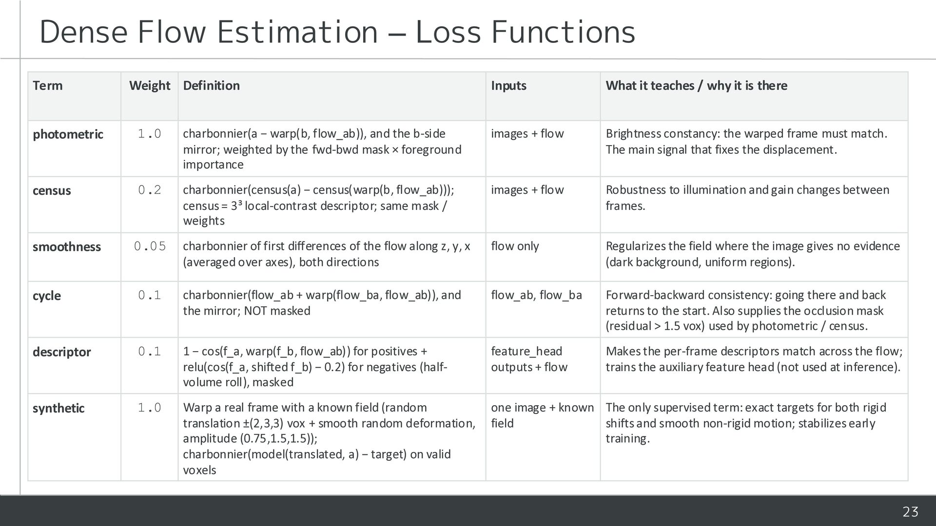
23. Dense Flow Estimation – Loss Functions Term Weight Definition Inputs What it teaches / why it is there photometric 1.0 charbonnier(a − warp(b, flow_ab)), and the b-side mirror; weighted by the fwd-bwd mask × foreground importance images + flow Brightness constancy: the warped frame must match. The main signal that fixes the displacement. census 0.2 charbonnier(census(a) − census(warp(b, flow_ab))); census = 3³ local-contrast descriptor; same mask / weights images + flow Robustness to illumination and gain changes between frames. smoothness 0.05 charbonnier of first differences of the flow along z, y, x (averaged over axes), both directions flow only Regularizes the field where the image gives no evidence (dark background, uniform regions). cycle 0.1 charbonnier(flow_ab + warp(flow_ba, flow_ab)), and the mirror; NOT masked flow_ab, flow_ba Forward-backward consistency: going there and back returns to the start. Also supplies the occlusion mask (residual > 1.5 vox) used by photometric / census. descriptor 0.1 1 − cos(f_a, warp(f_b, flow_ab)) for positives + relu(cos(f_a, shifted f_b) − 0.2) for negatives (halfvolume roll), masked feature_head outputs + flow Makes the per-frame descriptors match across the flow; trains the auxiliary feature head (not used at inference). synthetic 1.0 Warp a real frame with a known field (random translation ±(2,3,3) vox + smooth random deformation, amplitude (0.75,1.5,1.5)); charbonnier(model(translated, a) − target) on valid voxels one image + known The only supervised term: exact targets for both rigid field shifts and smooth non-rigid motion; stabilizes early training. 23
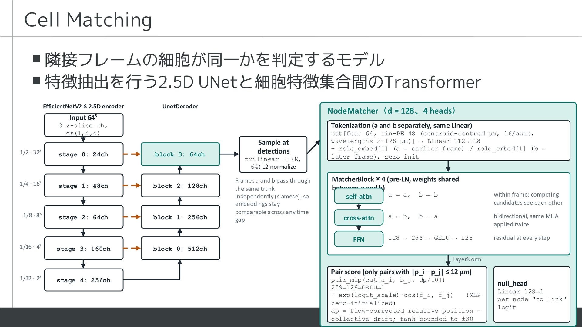
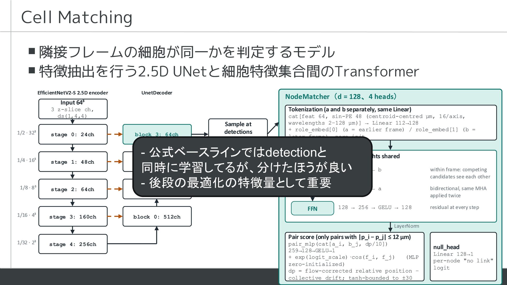
24. Cell Matching ▪ 隣接フレームの細胞が同一かを判定するモデル ▪ 特徴抽出を行う2.5D UNetと細胞特徴集合間のTransformer EfficientNetV2-S 2.5D encoder UnetDecoder NodeMatcher（d = 128、4 heads） Input 64³ 3 z-slice ch, ds(1,4,4) 1/2 · 32³ 1/4 · 16³ 1/8 · 8³ stage 0: 24ch stage 1: 48ch stage 2: 64ch Tokenization (a and b separately, same Linear) block 3: 64ch block 2: 128ch block 1: 256ch Sample at detections trilinear → (N, 64)L2-normalize Frames a and b pass through the same trunk independently (siamese), so embeddings stay comparable across any time gap cat[feat 64, sin-PE 48 (centroid-centred µm, 16/axis, wavelengths 2–128 µm)] → Linear 112→128 + role_embed[0] (a = earlier frame) / role_embed[1] (b = later frame), zero init MatcherBlock × 4 (pre-LN, weights shared between a and b) a ← a, b ← b self-attn cross-attn FFN 1/16 · 4³ stage 3: 160ch a ← b, within frame: competing candidates see each other b ← a bidirectional, same MHA applied twice 128 → 256 → GELU → 128 residual at every step block 0: 512ch LayerNorm 1/32 · 2³ Pair score (only pairs with |p_i − p_j| ≤ 12 µm) stage 4: 256ch pair_mlp(cat[a_i, b_j, dp/10]) 259→128→GELU→1 + exp(logit_scale)·cos(f_i, f_j) (MLP zero-initialized) dp = flow-corrected relative position − collective drift; tanh-bounded to ±30 null_head Linear 128→1 per-node "no link" logit 24
25. Cell Matching ▪ 隣接フレームの細胞が同一かを判定するモデル ▪ 特徴抽出を行う2.5D UNetと細胞特徴集合間のTransformer EfficientNetV2-S 2.5D encoder UnetDecoder NodeMatcher（d = 128、4 heads） Input 64³ 3 z-slice ch, ds(1,4,4) 1/2 · 32³ 1/4 · 16³ 1/8 · 8³ stage 0: 24ch stage 1: 48ch stage 2: 64ch Tokenization (a and b separately, same Linear) block 3: 64ch Sample at detections trilinear → (N, 64)L2-normalize cat[feat 64, sin-PE 48 (centroid-centred µm, 16/axis, wavelengths 2–128 µm)] → Linear 112→128 + role_embed[0] (a = earlier frame) / role_embed[1] (b = later frame), zero init - 公式ベースラインではdetectionと MatcherBlock × 4 (pre-LN, weights shared Frames a and b pass through block 2: 128ch between a and b) the same trunk a ← a, b ← b 同時に学習してるが、分けたほうが良い independently (siamese), so self-attn embeddings stay comparable across any time 後段の最適化の特徴量として重要 a ← b, b ← a block 1: 256ch cross-attn gap FFN 1/16 · 4³ stage 3: 160ch 128 → 256 → GELU → 128 within frame: competing candidates see each other bidirectional, same MHA applied twice residual at every step block 0: 512ch LayerNorm 1/32 · 2³ Pair score (only pairs with |p_i − p_j| ≤ 12 µm) stage 4: 256ch pair_mlp(cat[a_i, b_j, dp/10]) 259→128→GELU→1 + exp(logit_scale)·cos(f_i, f_j) (MLP zero-initialized) dp = flow-corrected relative position − collective drift; tanh-bounded to ±30 null_head Linear 128→1 per-node "no link" logit 25
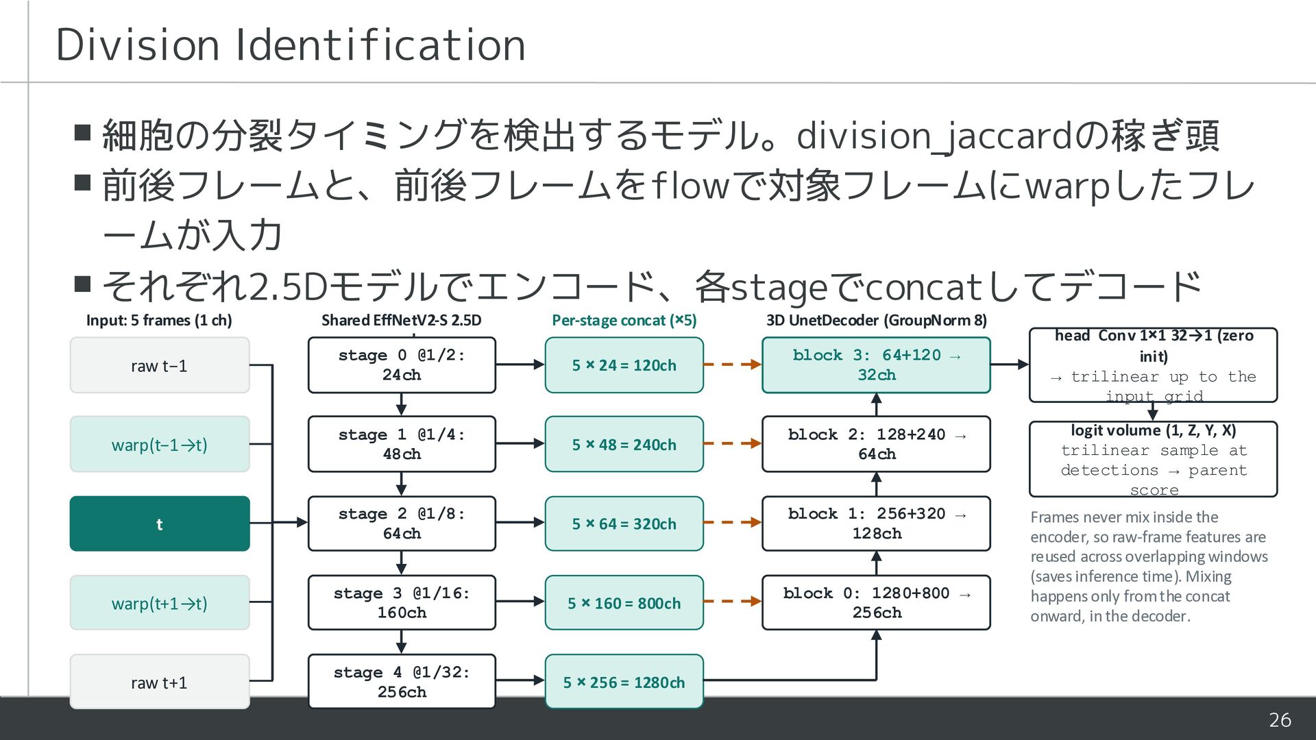
26. Division Identification ▪ 細胞の分裂タイミングを検出するモデル。division_jaccardの稼ぎ頭 ▪ 前後フレームと、前後フレームをflowで対象フレームにwarpしたフレ ームが入力 ▪ それぞれ2.5Dモデルでエンコード、各stageでconcatしてデコード Input: 5 frames (1 ch) raw t−1 Shared EffNetV2-S 2.5D encoder stage 0 @1/2: 24ch Per-stage concat (×5) 3D UnetDecoder (GroupNorm 8) 5 × 24 = 120ch block 3: 64+120 → 32ch warp(t−1→t) stage 1 @1/4: 48ch 5 × 48 = 240ch block 2: 128+240 → 64ch logit volume (1, Z, Y, X) trilinear sample at detections → parent score t stage 2 @1/8: 64ch 5 × 64 = 320ch block 1: 256+320 → 128ch block 0: 1280+800 → 256ch Frames never mix inside the encoder, so raw-frame features are reused across overlapping windows (saves inference time). Mixing happens only from the concat onward, in the decoder. warp(t+1→t) stage 3 @1/16: 160ch 5 × 160 = 800ch raw t+1 stage 4 @1/32: 256ch 5 × 256 = 1280ch head Conv 1×1 32→1 (zero init) → trilinear up to the input grid 26
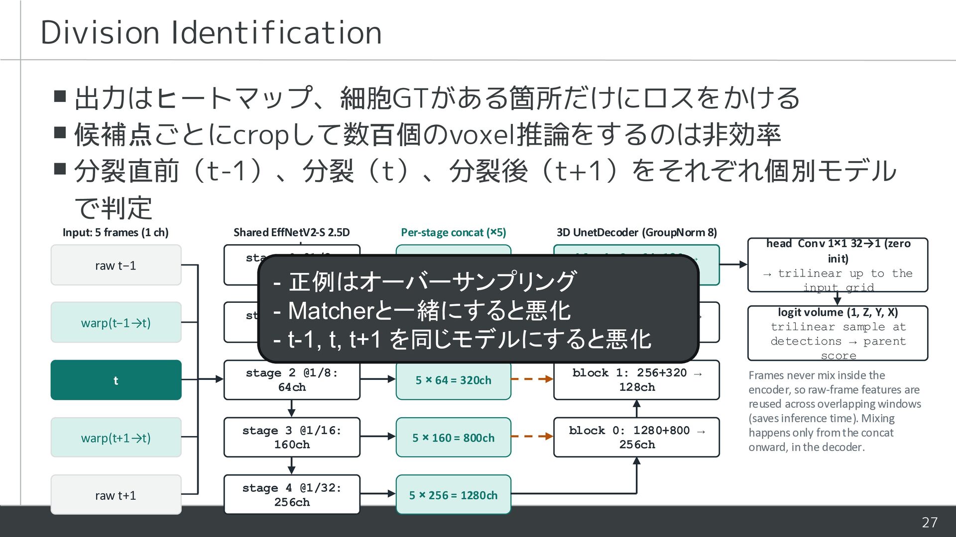
27. Division Identification ▪ 出力はヒートマップ、細胞GTがある箇所だけにロスをかける ▪ 候補点ごとにcropして数百個のvoxel推論をするのは非効率 ▪ 分裂直前（t-1）、分裂（t）、分裂後（t+1）をそれぞれ個別モデル で判定 Input: 5 frames (1 ch) raw t−1 warp(t−1→t) Shared EffNetV2-S 2.5D encoder stage 0 @1/2: 24ch Per-stage concat (×5) 3D UnetDecoder (GroupNorm 8) 5 × 24 = 120ch block 3: 64+120 → 32ch - 正例はオーバーサンプリング stage - Matcherと一緒にすると悪化 1 @1/4: block 2: 128+240 → 5 × 48 = 240ch 48ch 64ch - t-1, t, t+1 を同じモデルにすると悪化 t stage 2 @1/8: 64ch 5 × 64 = 320ch block 1: 256+320 → 128ch warp(t+1→t) stage 3 @1/16: 160ch 5 × 160 = 800ch block 0: 1280+800 → 256ch raw t+1 stage 4 @1/32: 256ch 5 × 256 = 1280ch head Conv 1×1 32→1 (zero init) → trilinear up to the input grid logit volume (1, Z, Y, X) trilinear sample at detections → parent score Frames never mix inside the encoder, so raw-frame features are reused across overlapping windows (saves inference time). Mixing happens only from the concat onward, in the decoder. 27
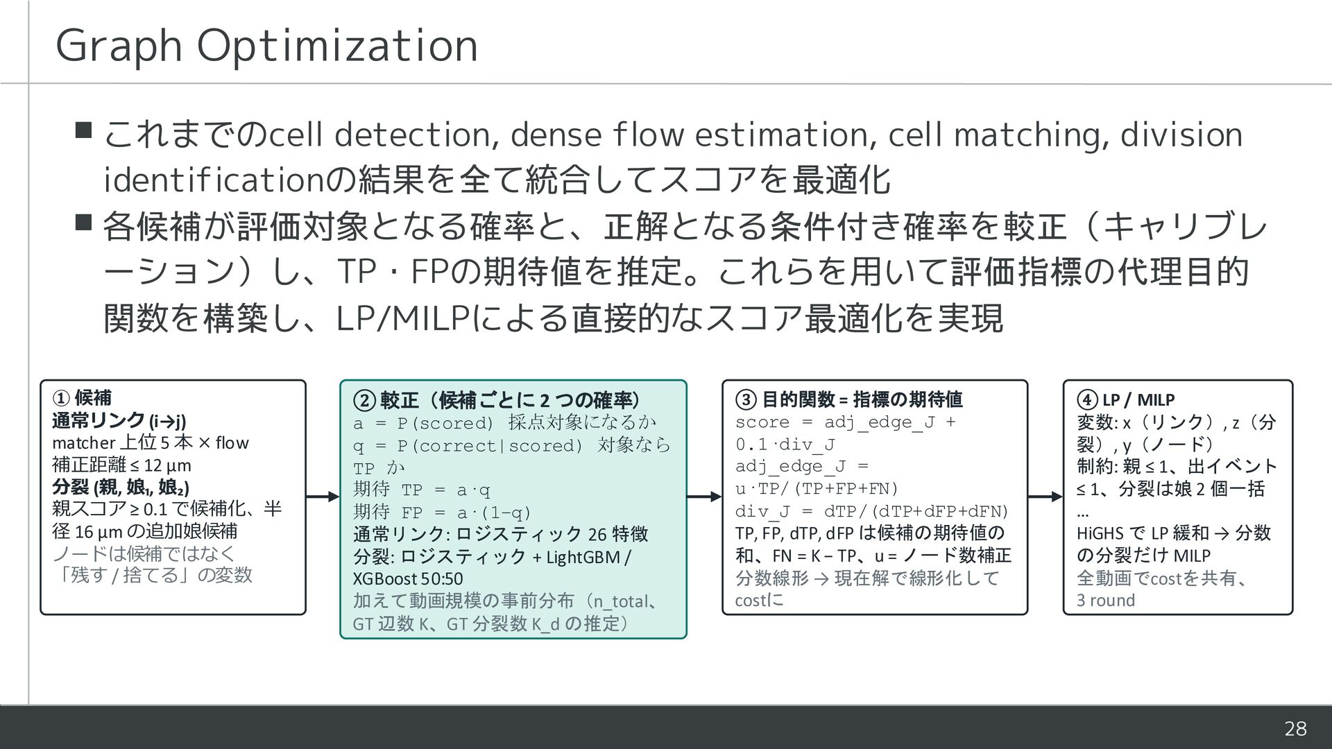
28. Graph Optimization ▪ これまでのcell detection, dense flow estimation, cell matching, division identificationの結果を全て統合してスコアを最適化 ▪ 各候補が評価対象となる確率と、正解となる条件付き確率を較正（キャリブレ ーション）し、TP・FPの期待値を推定。これらを用いて評価指標の代理目的 関数を構築し、LP/MILPによる直接的なスコア最適化を実現 ① 候補 通常リンク (i→j) matcher 上位 5 本 × flow 補正距離 ≤ 12 µm 分裂 (親, 娘₁, 娘₂) 親スコア ≥ 0.1 で候補化、半 径 16 µm の追加娘候補 ノードは候補ではなく 「残す / 捨てる」の変数 ② 較正（候補ごとに 2 つの確率） a = P(scored) 採点対象になるか q = P(correct|scored) 対象なら TP か 期待 TP = a·q 期待 FP = a·(1−q) 通常リンク: ロジスティック 26 特徴 分裂: ロジスティック + LightGBM / XGBoost 50:50 加えて動画規模の事前分布（n_total、 GT 辺数 K、GT 分裂数 K_d の推定） ③ 目的関数 = 指標の期待値 score = adj_edge_J + 0.1·div_J adj_edge_J = u·TP/(TP+FP+FN) div_J = dTP/(dTP+dFP+dFN) TP, FP, dTP, dFP は候補の期待値の 和、FN = K − TP、u = ノード数補正 分数線形 → 現在解で線形化して costに ④ LP / MILP 変数: x（リンク）, z（分 裂）, y（ノード） 制約: 親 ≤ 1、出イベント ≤ 1、分裂は娘 2 個一括 … HiGHS で LP 緩和 → 分数 の分裂だけ MILP 全動画でcostを共有、 3 round 28
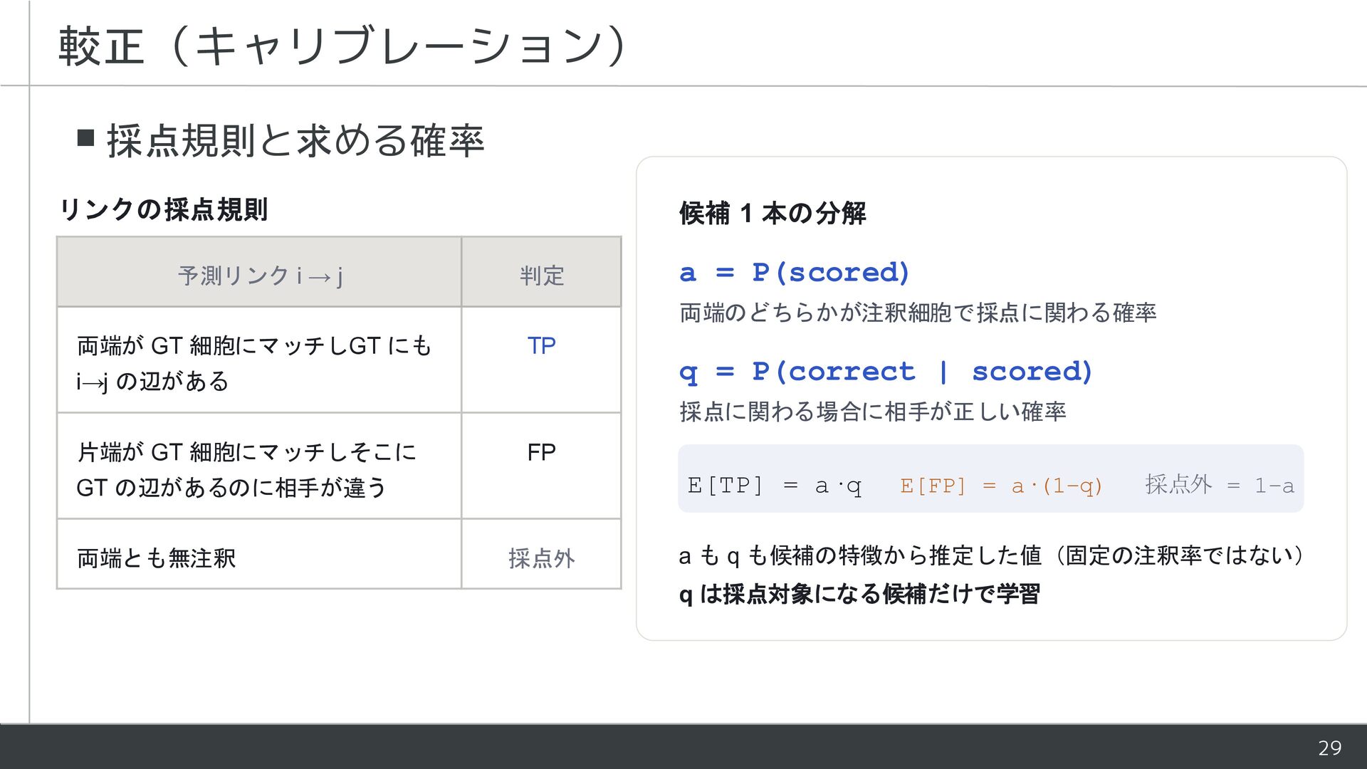
29. 較正（キャリブレーション） ▪ 採点規則と求める確率 リンクの採点規則 予測リンク → j 候補 1 本の分解 判定 a = P(scored) 両端のどちらかが注釈細胞で採点に関わる確率 両端が GT 細胞にマッチしGT にも TP →j の辺がある q = P(correct | scored) 採点に関わる場合に相手が正しい確率 片端が GT 細胞にマッチしそこに FP E[TP] = a·q GT の辺があるのに相手が違う 両端とも無注釈 採点外 E[FP] = a·(1−q) 採点外 = 1−a a も q も候補の特徴から推定した値（固定の注釈率ではない） q は採点対象になる候補だけで学習 29
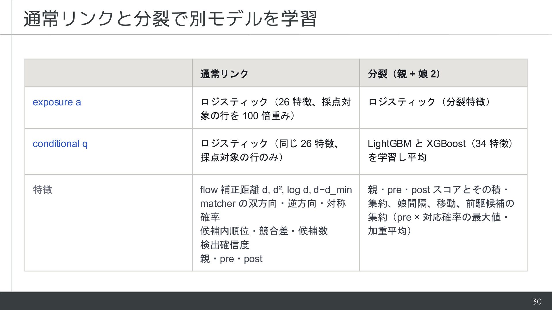
30. 通常リンクと分裂で別モデルを学習 通常リンク 分裂（親 + 娘 2） exposure a ロジスティック（26 特徴、採点対 象の行を 100 倍重み） ロジスティック（分裂特徴） conditional q ロジスティック（同じ 26 特徴、 採点対象の行のみ） LightGBM と XGBoost（34 特徴） を学習し平均 特徴 flow 補正距離 , ², l , −d_min matcher の双方向・逆方向・対称 確率 候補内順位・競合差・候補数 検出確信度 親・pre・post 親・pre・post スコアとその積・ 集約、娘間隔、移動、前駆候補の 集約（pre × 対応確率の最大値・ 加重平均） 30
31. Post-Processing ▪ Gap closing: 信頼性のあるリンク間の欠損を埋める ▪ 座標補正：globalの動きを推定しそれに合わせて座標を微修正 ▪ 短成分除去：6ノード未満のトラックを削除 座標補正 （点線→太線） Gap closing 短成分除去 t0 t1 t2 t3 t4 t5 t6 t7 t8 t9 31
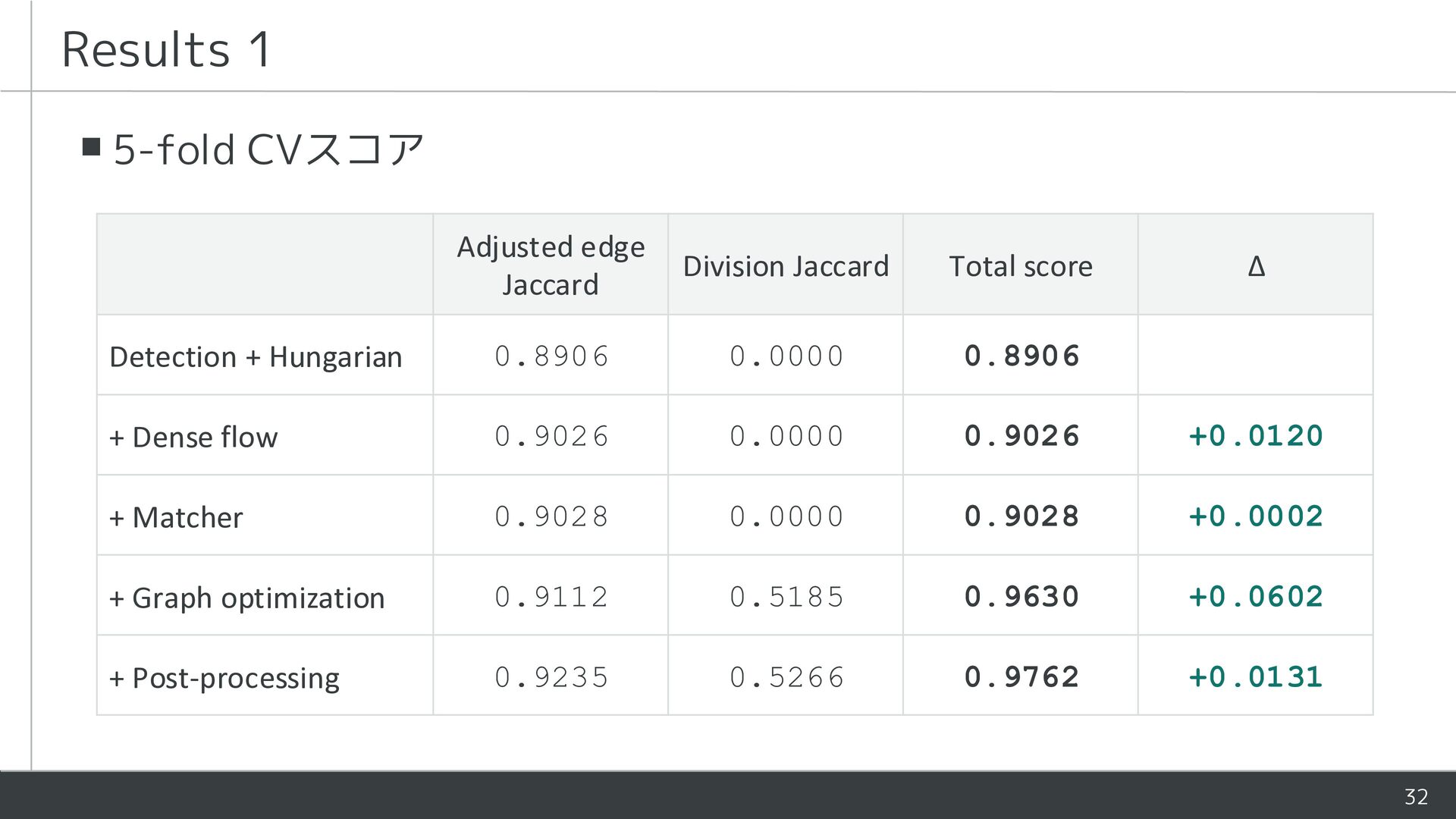
32. Results 1 ▪ 5-fold CVスコア Adjusted edge Jaccard Division Jaccard Total score Δ Detection + Hungarian 0.8906 0.0000 0.8906 — + Dense flow 0.9026 0.0000 0.9026 +0.0120 + Matcher 0.9028 0.0000 0.9028 +0.0002 + Graph optimization 0.9112 0.5185 0.9630 +0.0602 + Post-processing 0.9235 0.5266 0.9762 +0.0131 32
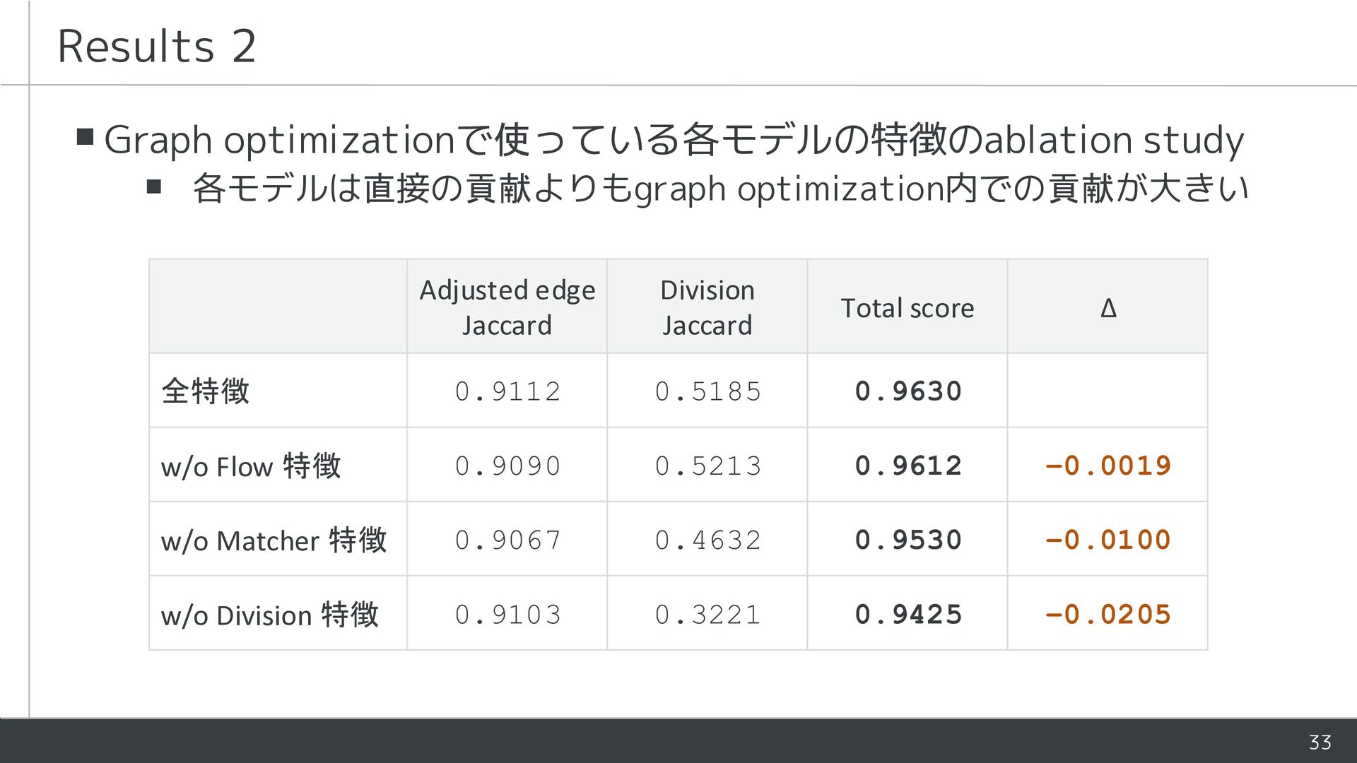
33. Results 2 ▪ Graph optimizationで使っている各モデルの特徴のablation study ▪ 各モデルは直接の貢献よりもgraph optimization内での貢献が大きい Adjusted edge Jaccard Division Jaccard Total score Δ 全特徴 0.9112 0.5185 0.9630 — w/o Flow 特徴 0.9090 0.5213 0.9612 −0.0019 w/o Matcher 特徴 0.9067 0.4632 0.9530 −0.0100 w/o Division 特徴 0.9103 0.3221 0.9425 −0.0205 33
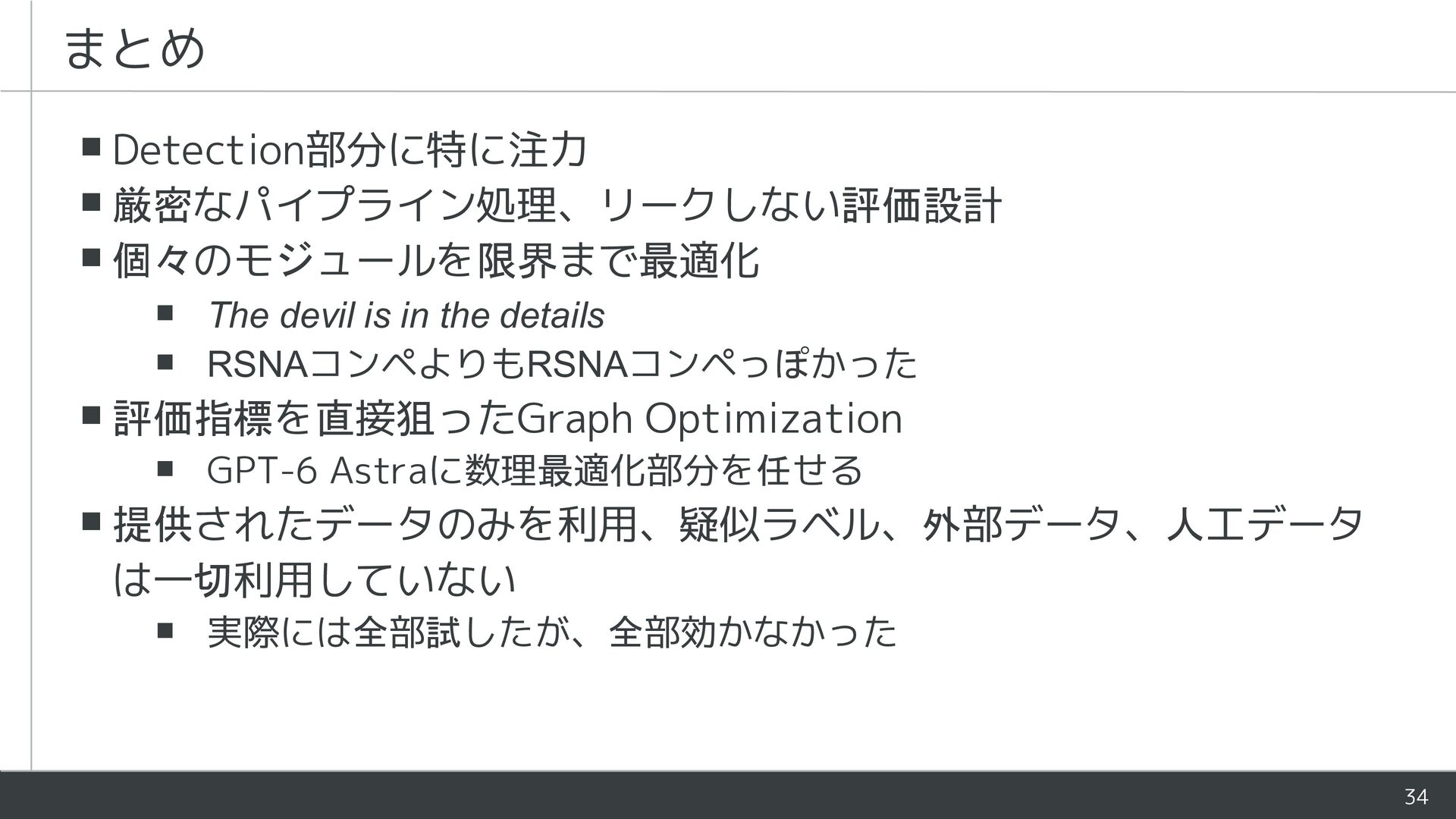
34. まとめ ▪ Detection部分に特に注力 ▪ 厳密なパイプライン処理、リークしない評価設計 ▪ 個々のモジュールを限界まで最適化 ▪ The devil is in the details ▪ RSNAコンペよりもRSNAコンペっぽかった ▪ 評価指標を直接狙ったGraph Optimization ▪ GPT-6 Astraに数理最適化部分を任せる ▪ 提供されたデータのみを利用、疑似ラベル、外部データ、人工データ は一切利用していない ▪ 実際には全部試したが、全部効かなかった 34