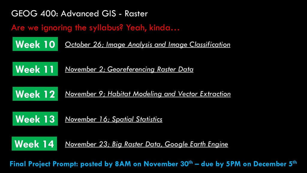
ignoring the syllabus? Yeah, kinda… October 26; Image Analysis and Image Classification Week 14 Week 11 Week 12 Week 13 November 23; Big Raster Data, Google Earth Engine November 2; Georeferencing Raster Data November 9; Habitat Modeling and Vector Extraction November 16; Spatial Statistics Final Project Prompt: posted by 8AM on November 30th – due by 5PM on December 5th
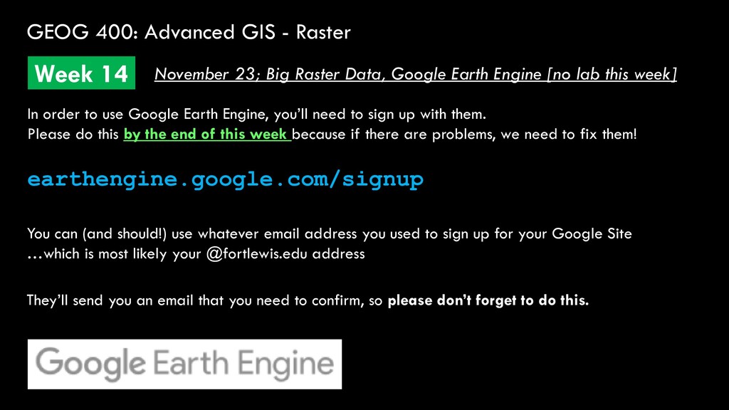
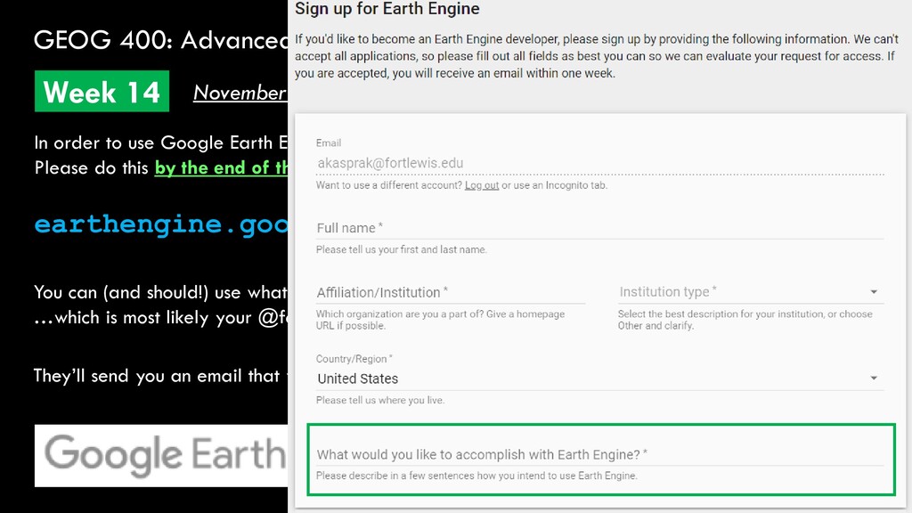
Big Raster Data, Google Earth Engine [no lab this week] In order to use Google Earth Engine, you’ll need to sign up with them. Please do this by the end of this week because if there are problems, we need to fix them! earthengine.google.com/signup You can (and should!) use whatever email address you used to sign up for your Google Site …which is most likely your @fortlewis.edu address They’ll send you an email that you need to confirm, so please don’t forget to do this.
Big Raster Data, Google Earth Engine [no lab this week] In order to use Google Earth Engine, you’ll need to sign up with them. Please do this by the end of this week because if there are problems, we need to fix them! earthengine.google.com/signup You can (and should!) use whatever email address you used to sign up for your Google Site …which is most likely your @fortlewis.edu address They’ll send you an email that you need to confirm, so please don’t forget to do this.
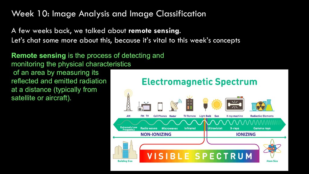
back, we talked about remote sensing. Let’s chat some more about this, because it’s vital to this week’s concepts Remote sensing is the process of detecting and monitoring the physical characteristics of an area by measuring its reflected and emitted radiation at a distance (typically from satellite or aircraft).
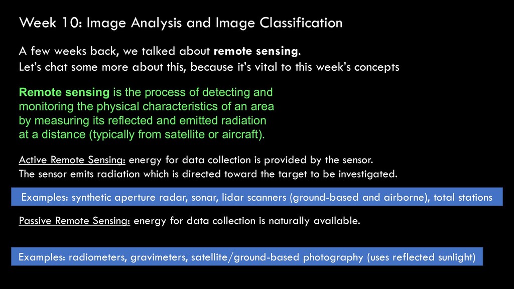
back, we talked about remote sensing. Let’s chat some more about this, because it’s vital to this week’s concepts Remote sensing is the process of detecting and monitoring the physical characteristics of an area by measuring its reflected and emitted radiation at a distance (typically from satellite or aircraft). Active Remote Sensing: energy for data collection is provided by the sensor. The sensor emits radiation which is directed toward the target to be investigated. Passive Remote Sensing: energy for data collection is naturally available. Examples: synthetic aperture radar, sonar, lidar scanners (ground-based and airborne), total stations Examples: radiometers, gravimeters, satellite/ground-based photography (uses reflected sunlight)
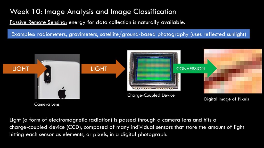
energy for data collection is naturally available. Examples: radiometers, gravimeters, satellite/ground-based photography (uses reflected sunlight) LIGHT LIGHT Camera Lens Charge-Coupled Device Digital Image of Pixels CONVERSION Light (a form of electromagnetic radiation) is passed through a camera lens and hits a charge-coupled device (CCD), composed of many individual sensors that store the amount of light hitting each sensor as elements, or pixels, in a digital photograph.
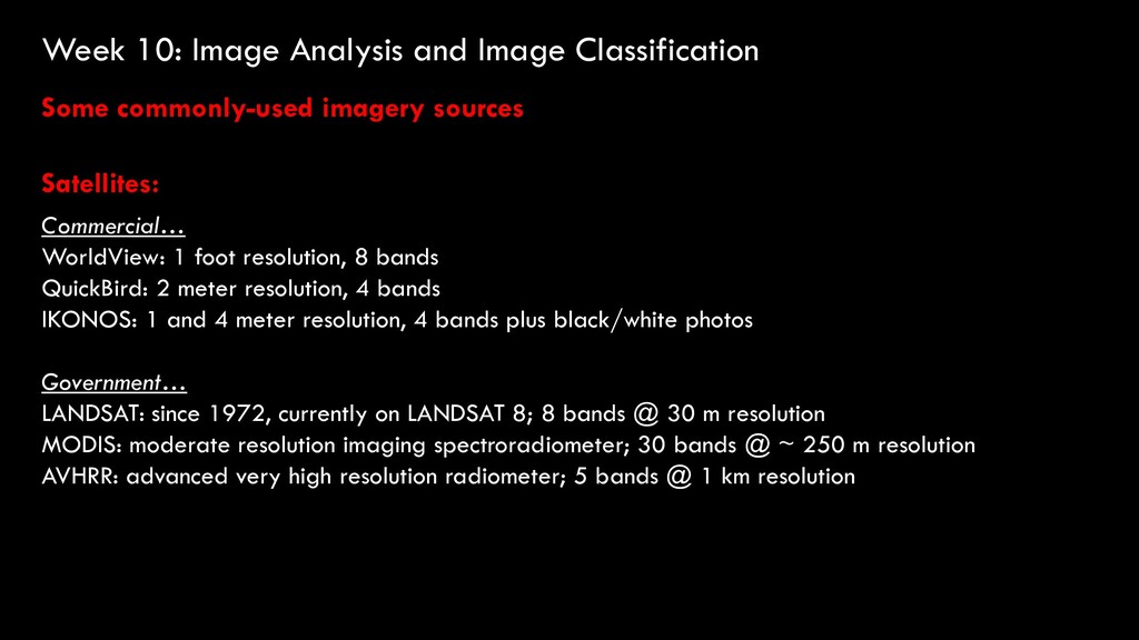
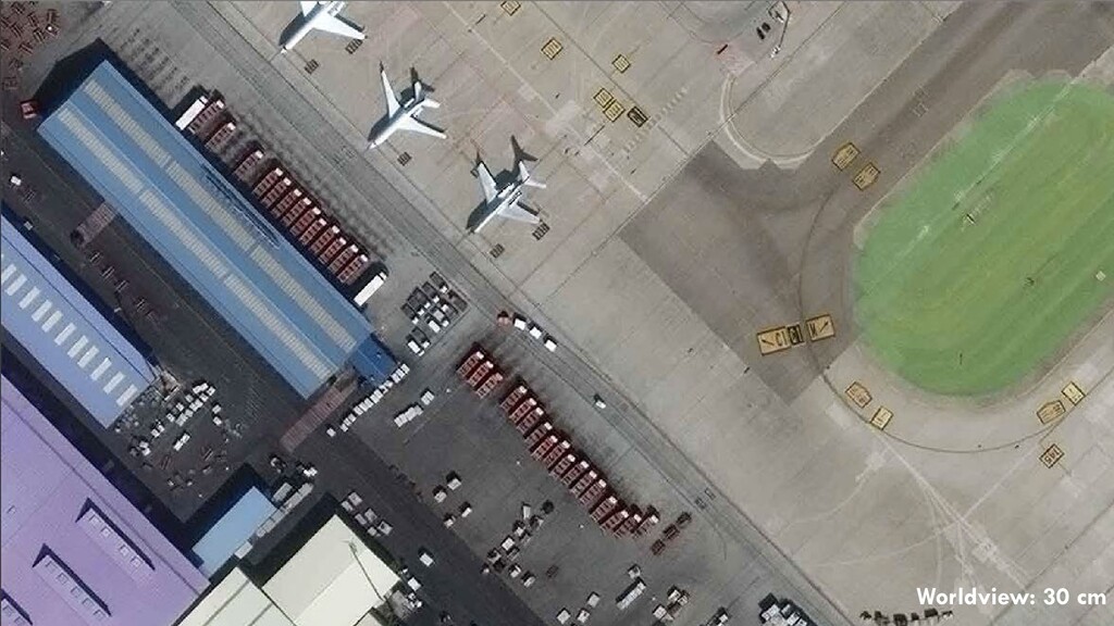
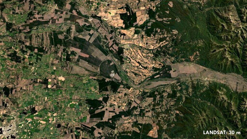
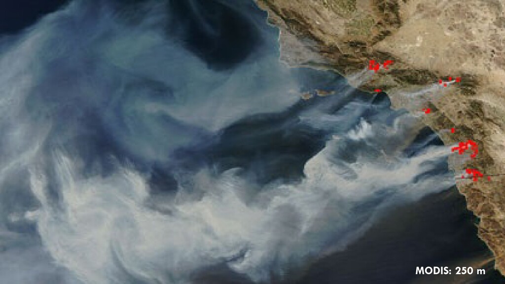
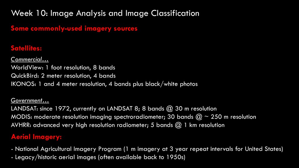
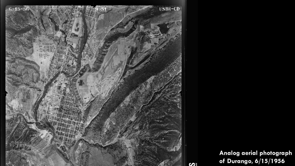
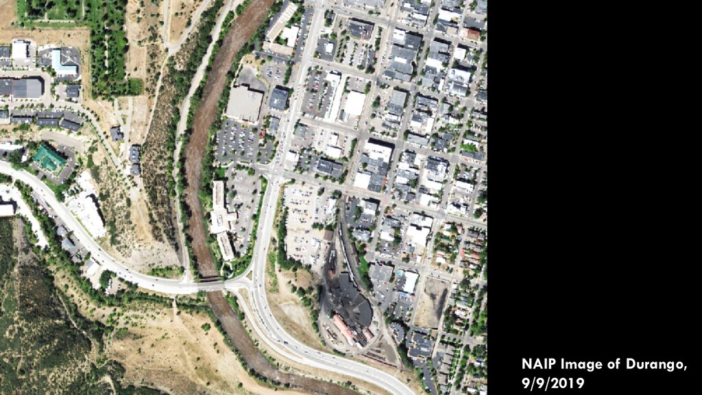
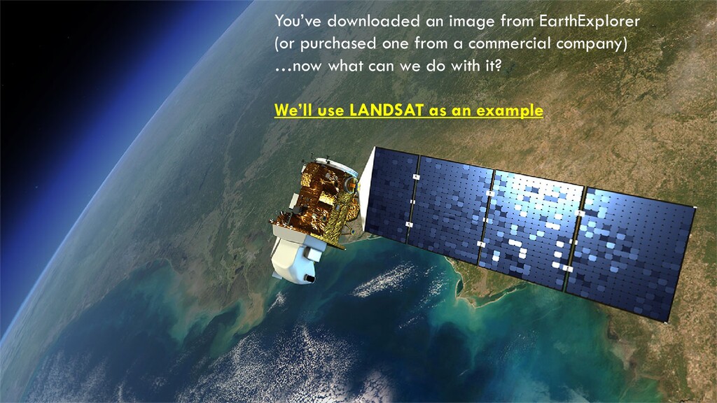
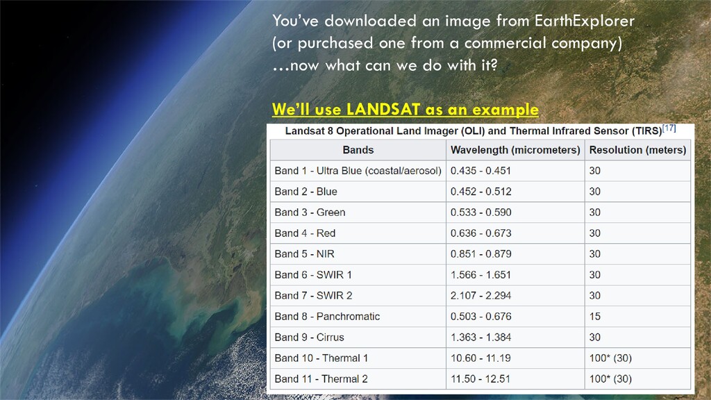
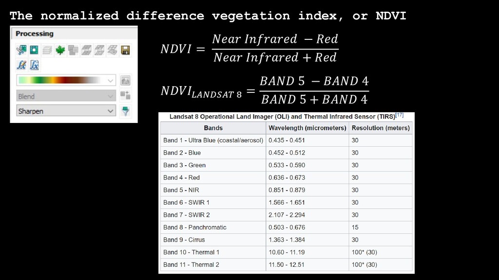
sources Satellites: Commercial… WorldView: 1 foot resolution, 8 bands QuickBird: 2 meter resolution, 4 bands IKONOS: 1 and 4 meter resolution, 4 bands plus black/white photos Government… LANDSAT: since 1972, currently on LANDSAT 8; 8 bands @ 30 m resolution MODIS: moderate resolution imaging spectroradiometer; 30 bands @ ~ 250 m resolution AVHRR: advanced very high resolution radiometer; 5 bands @ 1 km resolution Aerial Imagery: - National Agricultural Imagery Program (1 m imagery at 3 year repeat intervals for United States) - Legacy/historic aerial images (often available back to 1950s)
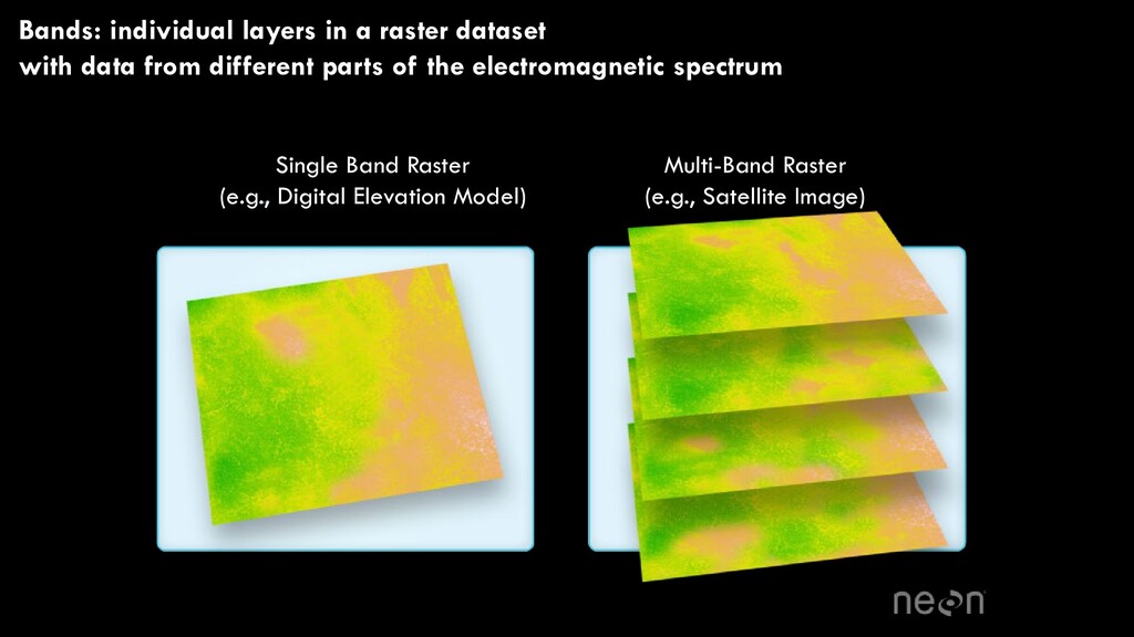
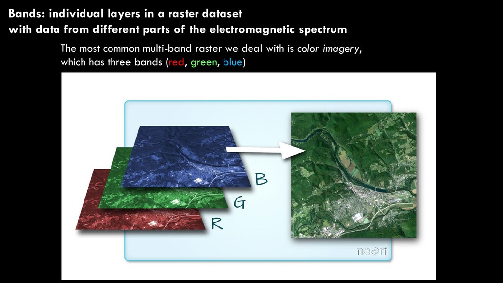
imagery, which has three bands (red, green, blue) Bands: individual layers in a raster dataset with data from different parts of the electromagnetic spectrum
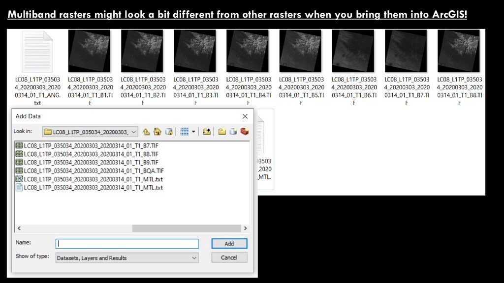
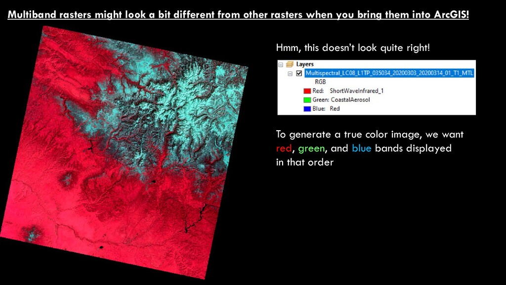
color image, we want red, green, and blue bands displayed in that order Multiband rasters might look a bit different from other rasters when you bring them into ArcGIS!
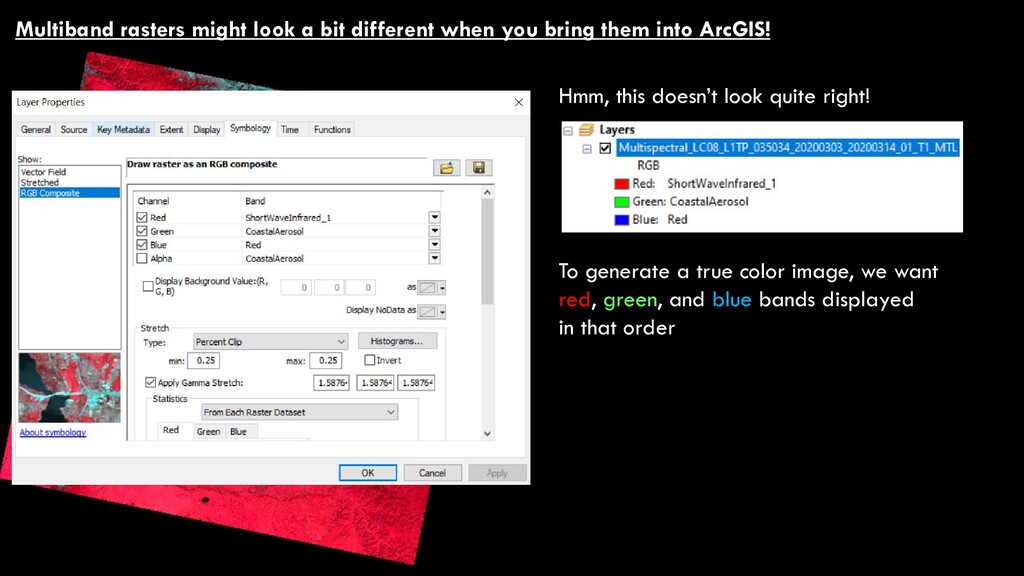
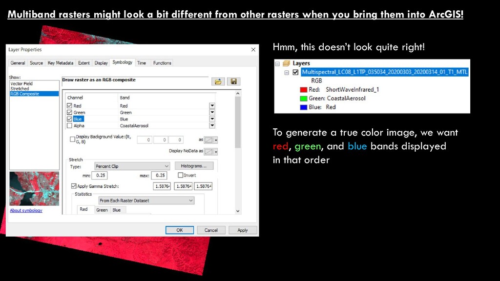
when you bring them into ArcGIS! Hmm, this doesn’t look quite right! To generate a true color image, we want red, green, and blue bands displayed in that order
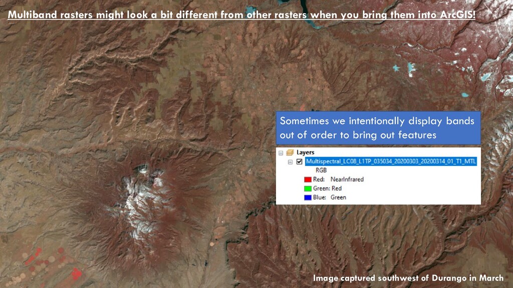
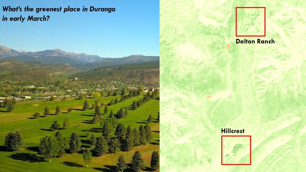
when you bring them into ArcGIS! Sometimes we intentionally display bands out of order to bring out features Image captured southwest of Durango in March
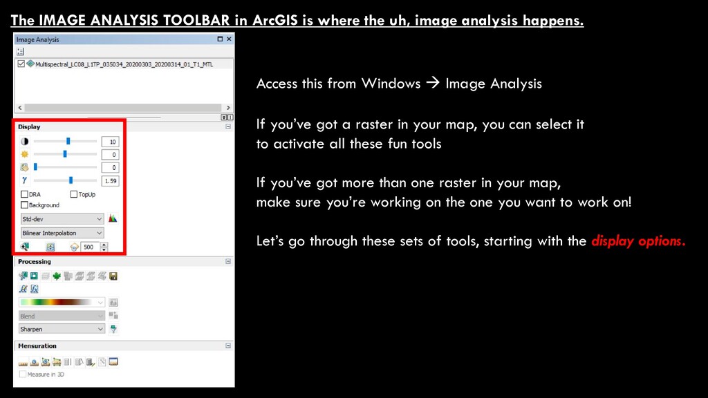
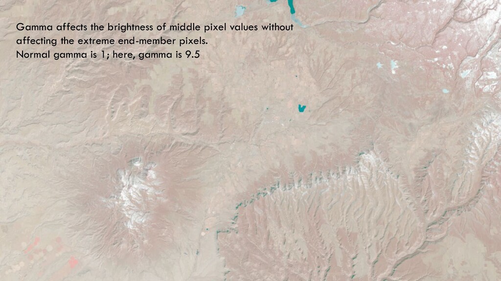
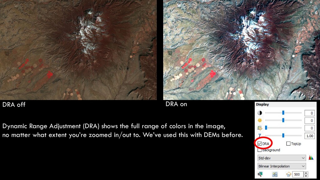
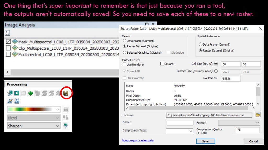
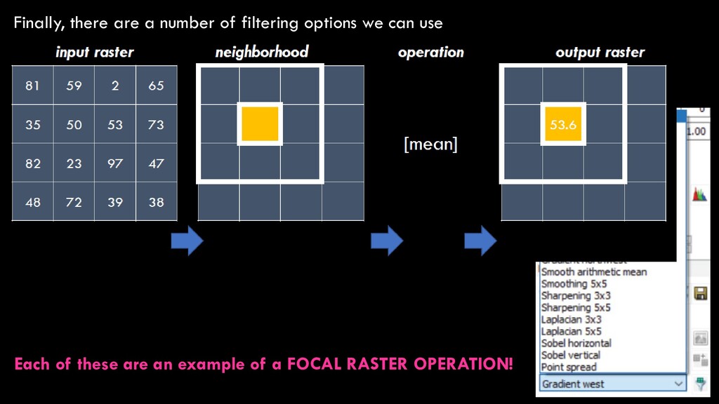
image analysis happens. Access this from Windows Image Analysis If you’ve got a raster in your map, you can select it to activate all these fun tools If you’ve got more than one raster in your map, make sure you’re working on the one you want to work on! Let’s go through these sets of tools, starting with the display options.
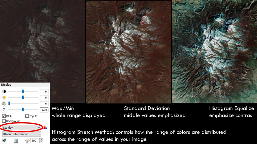
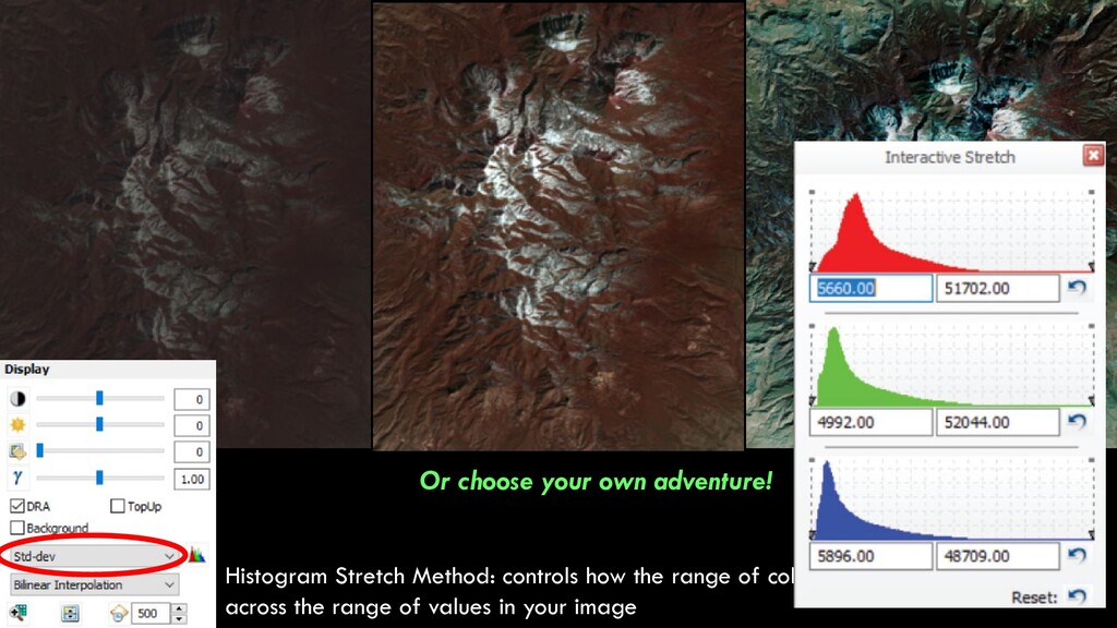
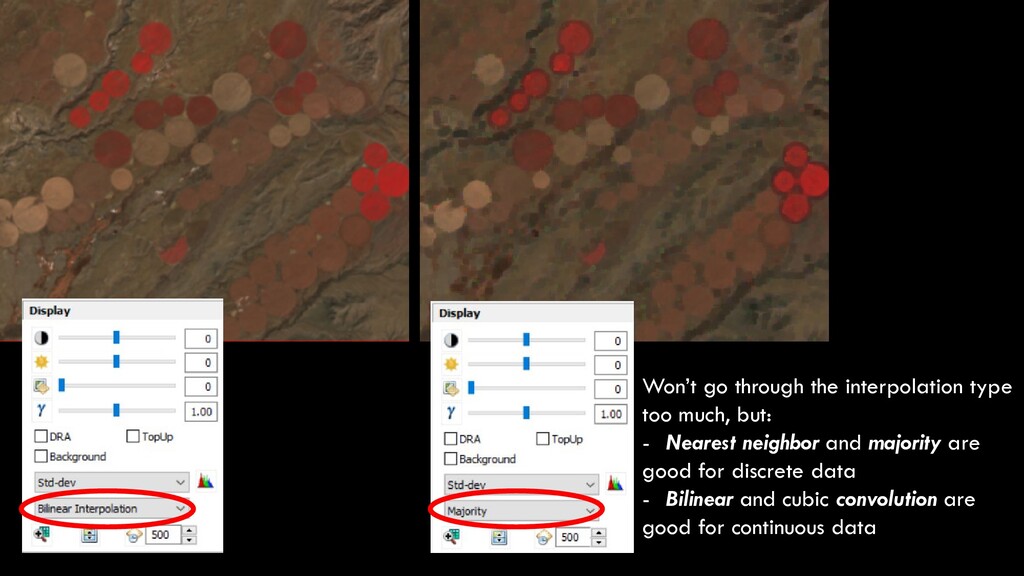
distributed across the range of values in your image Max/Min whole range displayed Standard Deviation middle values emphasized Histogram Equalize emphasize contras
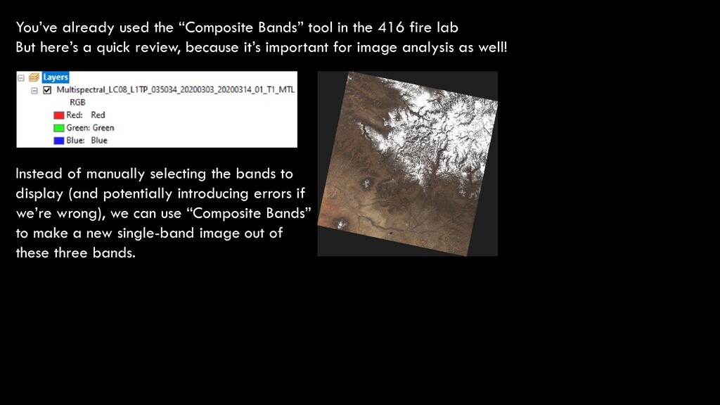
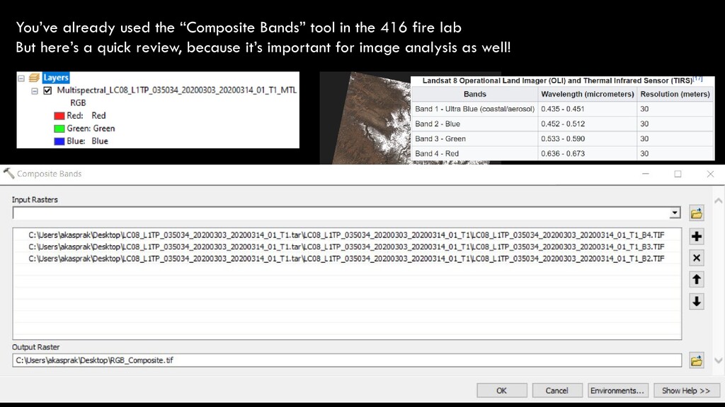
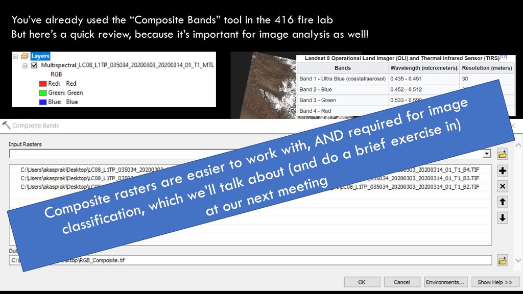
fire lab But here’s a quick review, because it’s important for image analysis as well! Instead of manually selecting the bands to display (and potentially introducing errors if we’re wrong), we can use “Composite Bands” to make a new single-band image out of these three bands.
fire lab But here’s a quick review, because it’s important for image analysis as well! Instead of manually selecting the bands to display (and potentially introducing errors if we’re wrong), we can use “Composite Bands” to make a new single-band image out of these three bands.
fire lab But here’s a quick review, because it’s important for image analysis as well! Instead of manually selecting the bands to display (and potentially introducing errors if we’re wrong), we can use “Composite Bands” to make a new single-band image out of these three bands.