CMNS201 - Lab 7. SPSS Multivariate Analysis

Transcript

1. Multivariate analysis in SPSS SPSS LABORATORY 7
2. 1. Calendar 2. Multivariate analysis and control variables: theory 3. Adding a control variable to your analysis in SPSS 4. Exercise INDEX
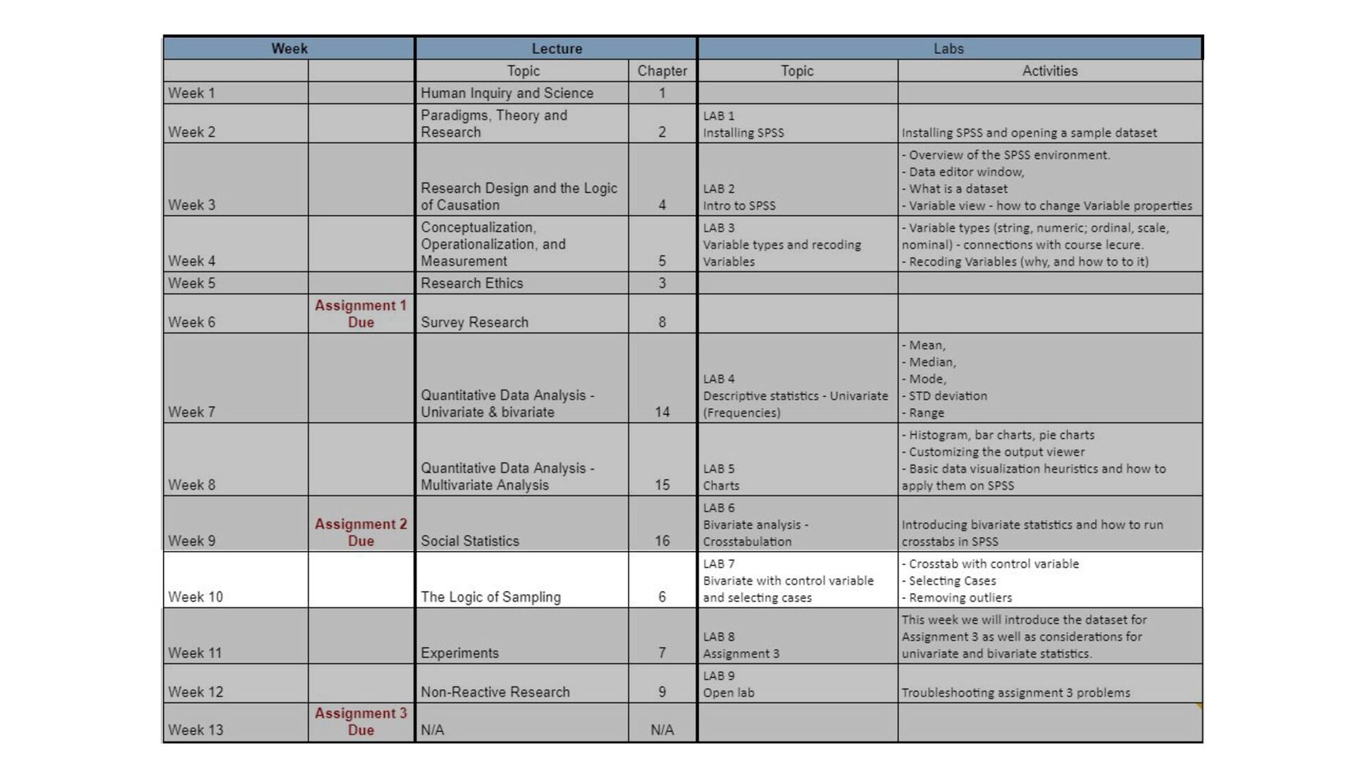
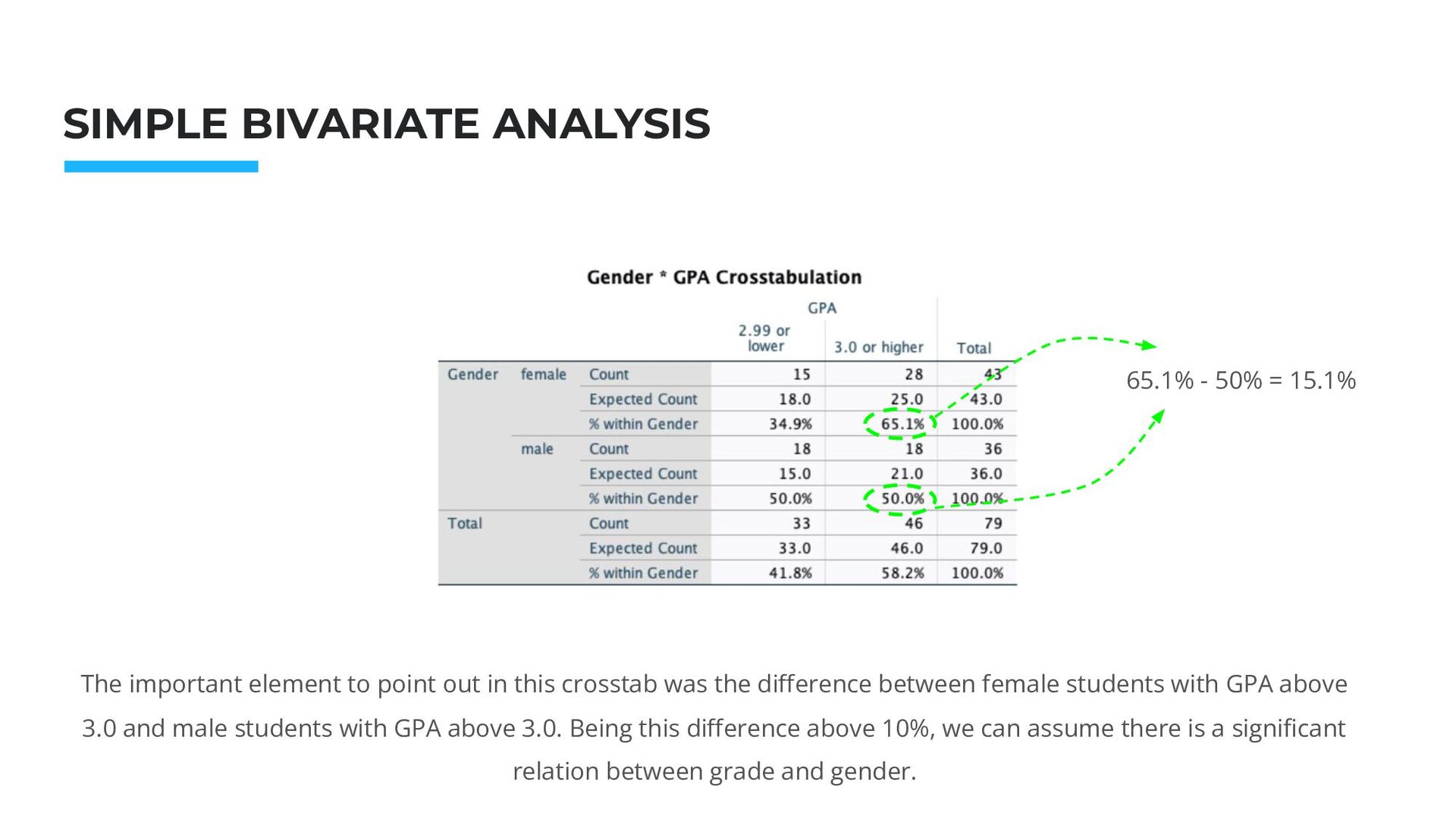
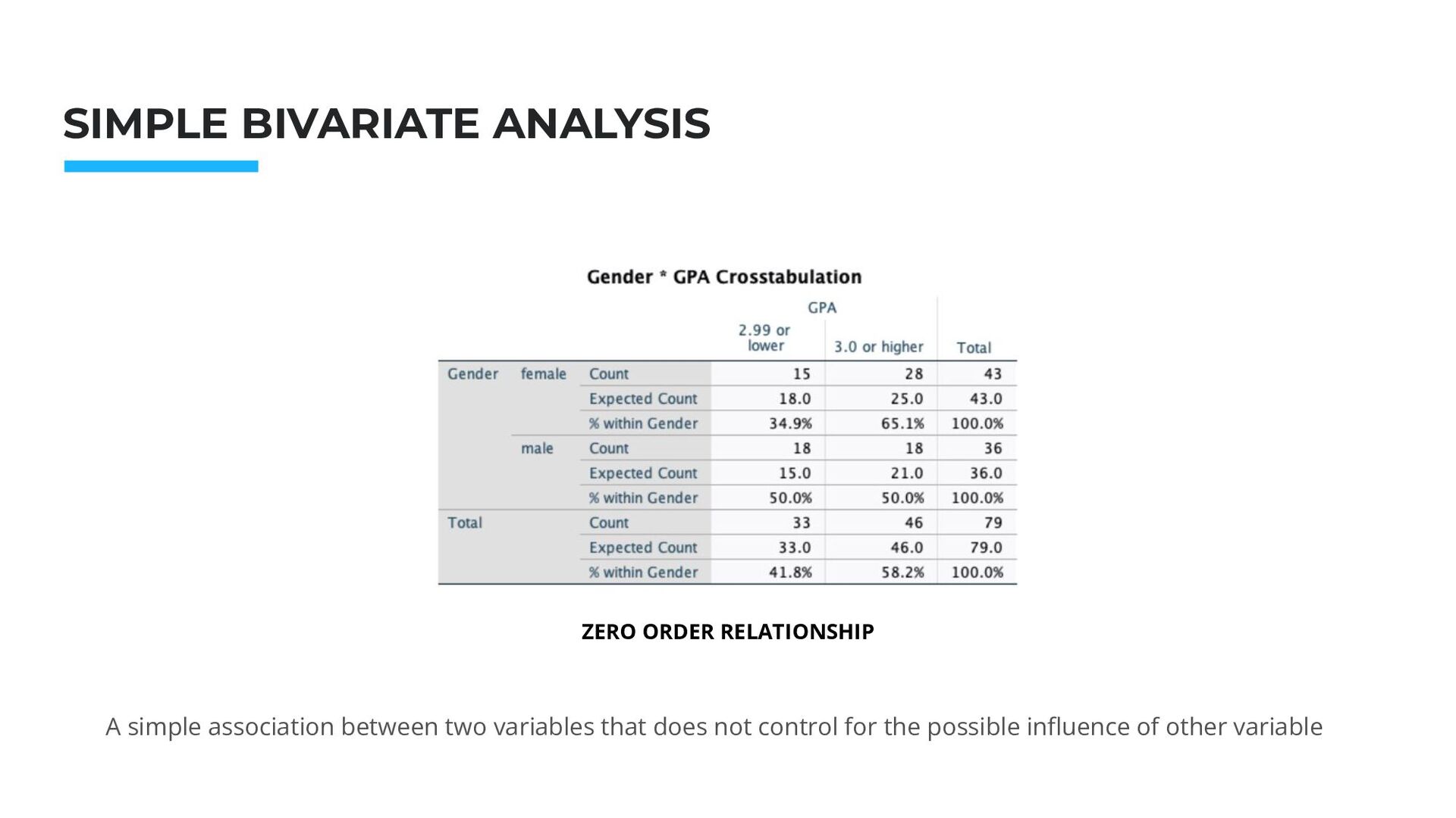
4. Photo: Startup Weekend Hackathon. Nov.2014 SIMPLE BIVARIATE ANALYSIS The important element to point out in this crosstab was the difference between female students with GPA above 3.0 and male students with GPA above 3.0. Being this difference above 10%, we can assume there is a significant relation between grade and gender. 65.1% - 50% = 15.1%
5. Photo: Startup Weekend Hackathon. Nov.2014 SIMPLE BIVARIATE ANALYSIS A simple association between two variables that does not control for the possible influence of other variable ZERO ORDER RELATIONSHIP
6. Photo: Startup Weekend Hackathon. Nov.2014 CONTROL VARIABLE A control variable is a variable which is held constant throughout a research in order to assess the relationship between dependent and independent variables. Since it remains constant, it enables researchers to test and better understand the relationship between dependent and independent variables.
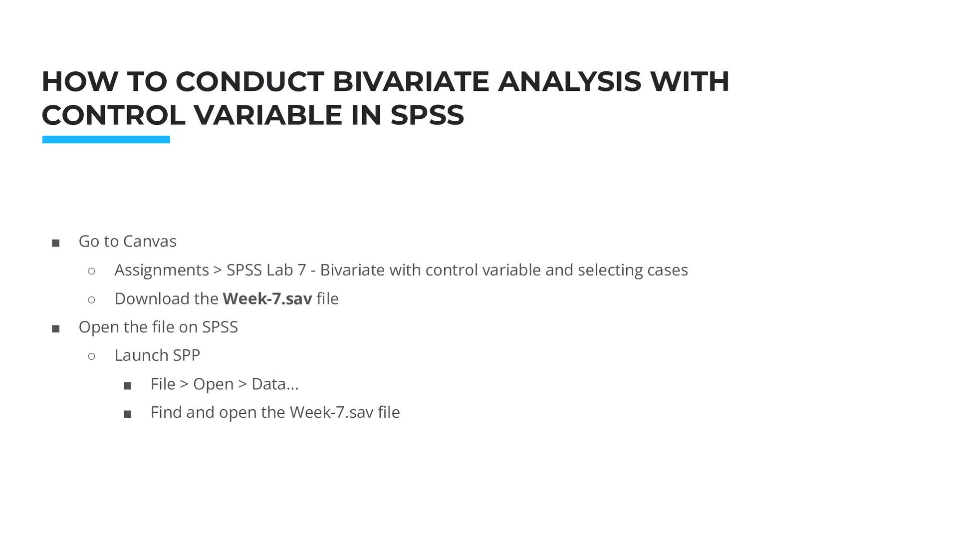
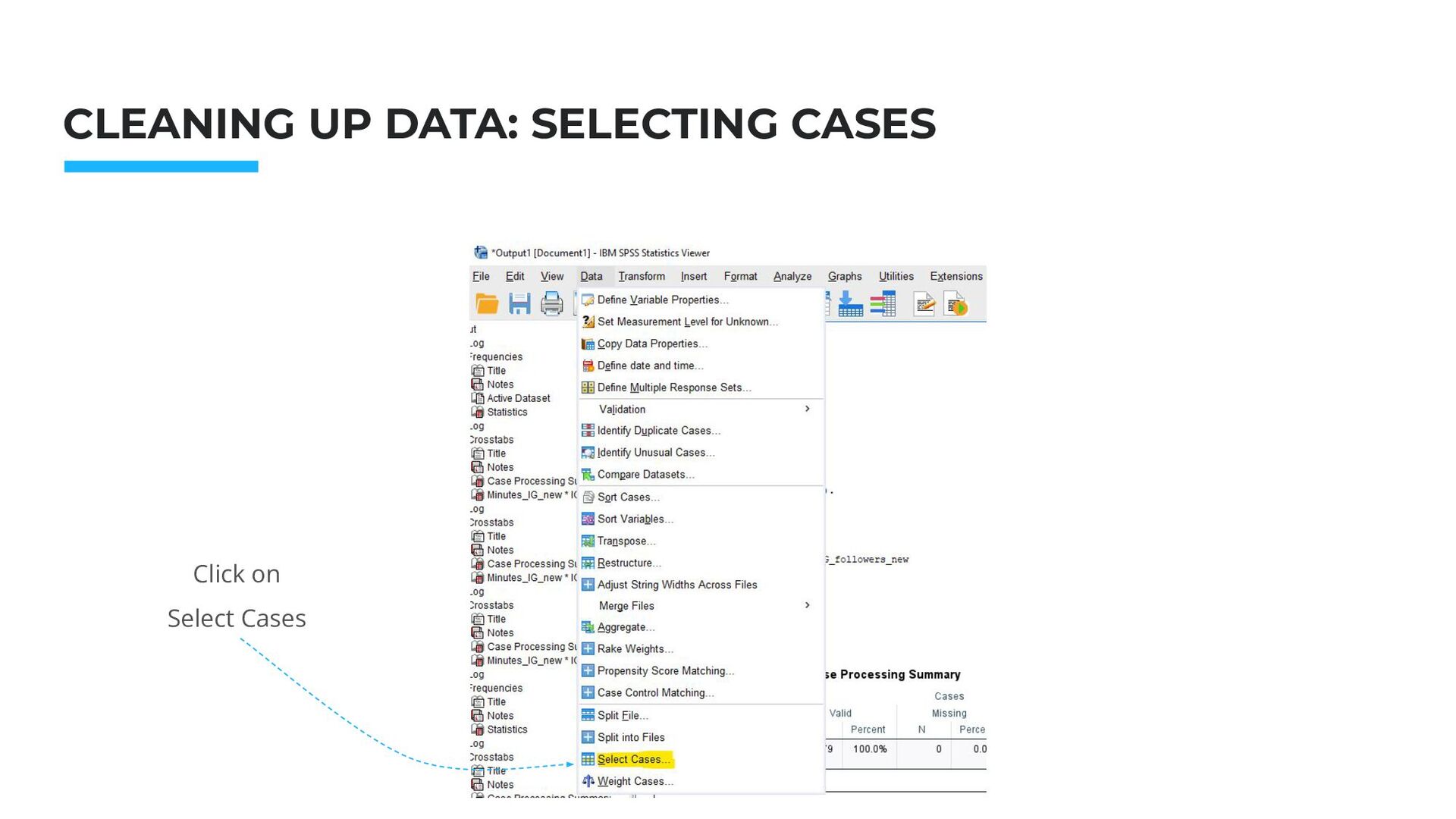
7. Photo: Startup Weekend Hackathon. Nov.2014 HOW TO CONDUCT BIVARIATE ANALYSIS WITH CONTROL VARIABLE IN SPSS ▪ Go to Canvas ◦ Assignments > SPSS Lab 7 - Bivariate with control variable and selecting cases ◦ Download the Week-7.sav file ▪ Open the file on SPSS ◦ Launch SPP ▪ File > Open > Data… ▪ Find and open the Week-7.sav file
8. Photo: Startup Weekend Hackathon. Nov.2014 AS USUAL, LET’S BEGIN WITH A HYPOTHESIS People who spend more time on Instagram will tend to have more followers than people who spend less time on it. Null hypothesis: there is no relationship between time spent on Instagram and number of followers
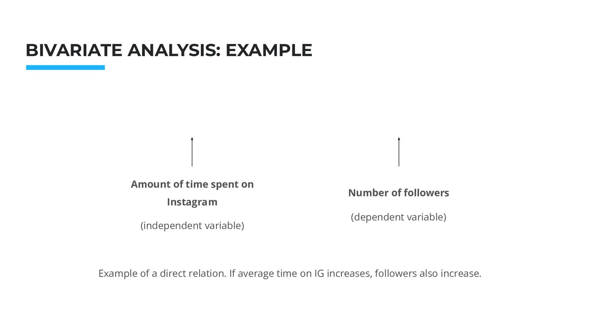
9. Photo: Startup Weekend Hackathon. Nov.2014 BIVARIATE ANALYSIS: EXAMPLE Amount of time spent on Instagram (independent variable) Number of followers (dependent variable) Example of a direct relation. If average time on IG increases, followers also increase.
10. Photo: Startup Weekend Hackathon. Nov.2014 PREPARING THE VARIABLES Amount of time spent on Instagram Number of followers Simplified, 2-value, nominal variable Simplified, 2-value, nominal variable
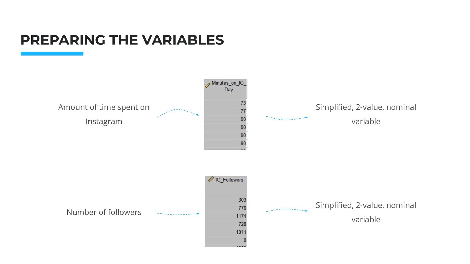
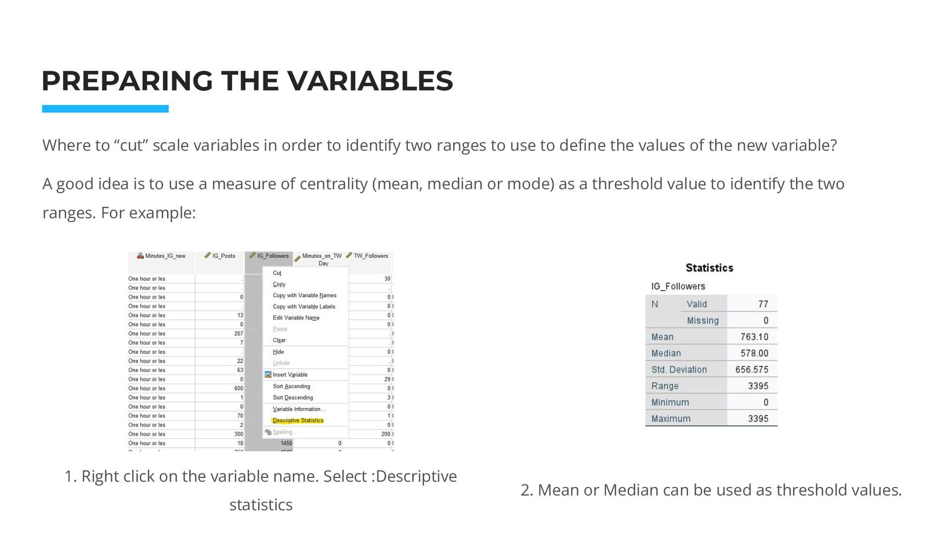
11. Photo: Startup Weekend Hackathon. Nov.2014 PREPARING THE VARIABLES Where to “cut” scale variables in order to identify two ranges to use to define the values of the new variable? A good idea is to use a measure of centrality (mean, median or mode) as a threshold value to identify the two ranges. For example: 1. Right click on the variable name. Select :Descriptive statistics 2. Mean or Median can be used as threshold values.
12. Photo: Startup Weekend Hackathon. Nov.2014 PREPARING THE VARIABLES Another option for identifying a threshold is to refer to arbitrary values that are meaningful in the context of the analysis. For example, in the case of this hypothesis, we can define people who use Instagram less than 1 hour a day as casual users, and people who use it for more than one hour a day as intense users. All arbitrary values are good threshold values as long as they are consistent with your hypothesis.
13. Photo: Startup Weekend Hackathon. Nov.2014 BIVARIATE ANALYSIS WITH RECODED VARIABLES
14. Photo: Startup Weekend Hackathon. Nov.2014 BIVARIATE ANALYSIS WITH RECODED VARIABLES Missing values
15. Photo: Startup Weekend Hackathon. Nov.2014 CLEANING UP DATA: SELECTING CASES Click on Select Cases
16. Photo: Startup Weekend Hackathon. Nov.2014 CLEANING UP DATA: SELECTING CASES 1. Click on If condition is satisfied 2. Click If… button
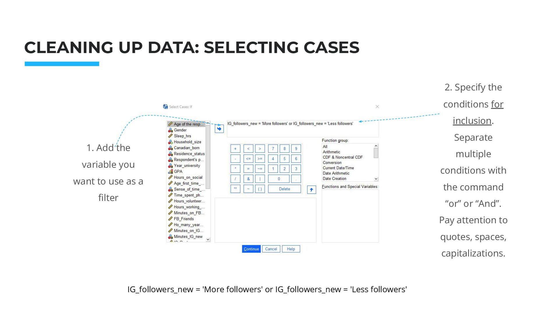
17. Photo: Startup Weekend Hackathon. Nov.2014 CLEANING UP DATA: SELECTING CASES 1. Add the variable you want to use as a filter 2. Specify the conditions for inclusion. Separate multiple conditions with the command “or” or “And”. Pay attention to quotes, spaces, capitalizations. IG_followers_new = 'More followers' or IG_followers_new = 'Less followers'
18. Photo: Startup Weekend Hackathon. Nov.2014 CLEANING UP DATA: SELECTING CASES
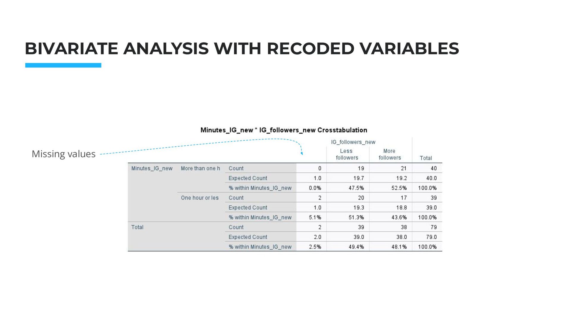
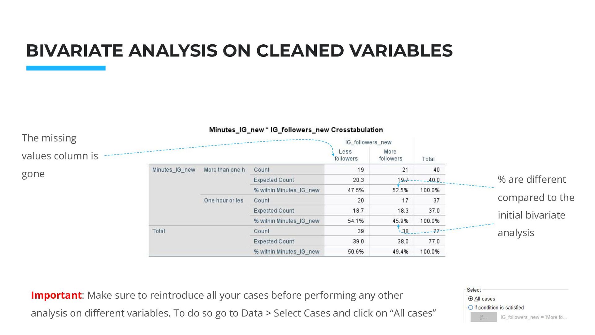
19. Photo: Startup Weekend Hackathon. Nov.2014 BIVARIATE ANALYSIS ON CLEANED VARIABLES The missing values column is gone % are different compared to the initial bivariate analysis Important: Make sure to reintroduce all your cases before performing any other analysis on different variables. To do so go to Data > Select Cases and click on “All cases”
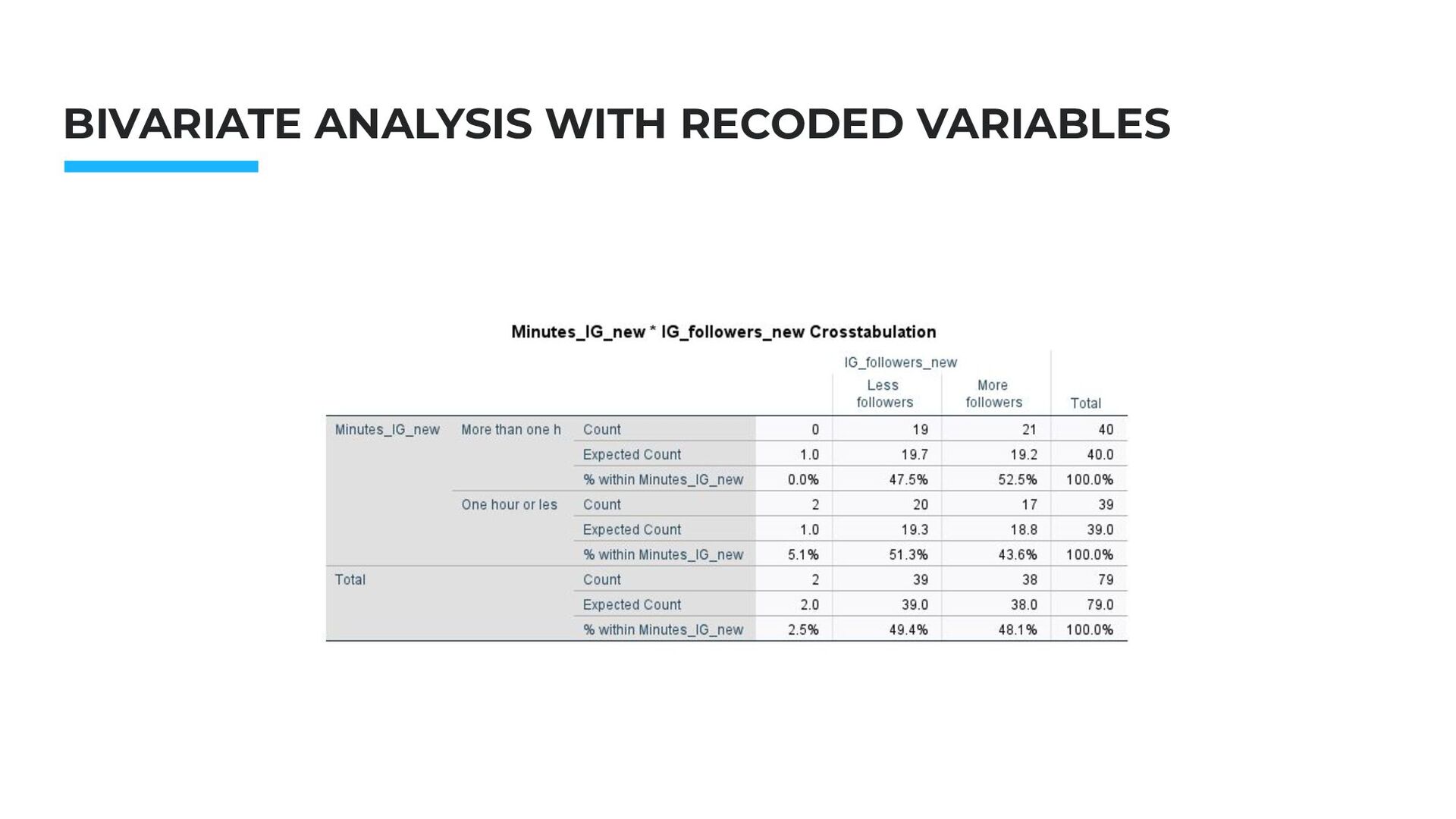
20. Photo: Startup Weekend Hackathon. Nov.2014 CROSSTAB INTERPRETATION Since the difference between % is less than 10%, we can conclude that the data do not support our the hypothesis. The Null hypothesis is true: there is no relation between independent and dependent variable.
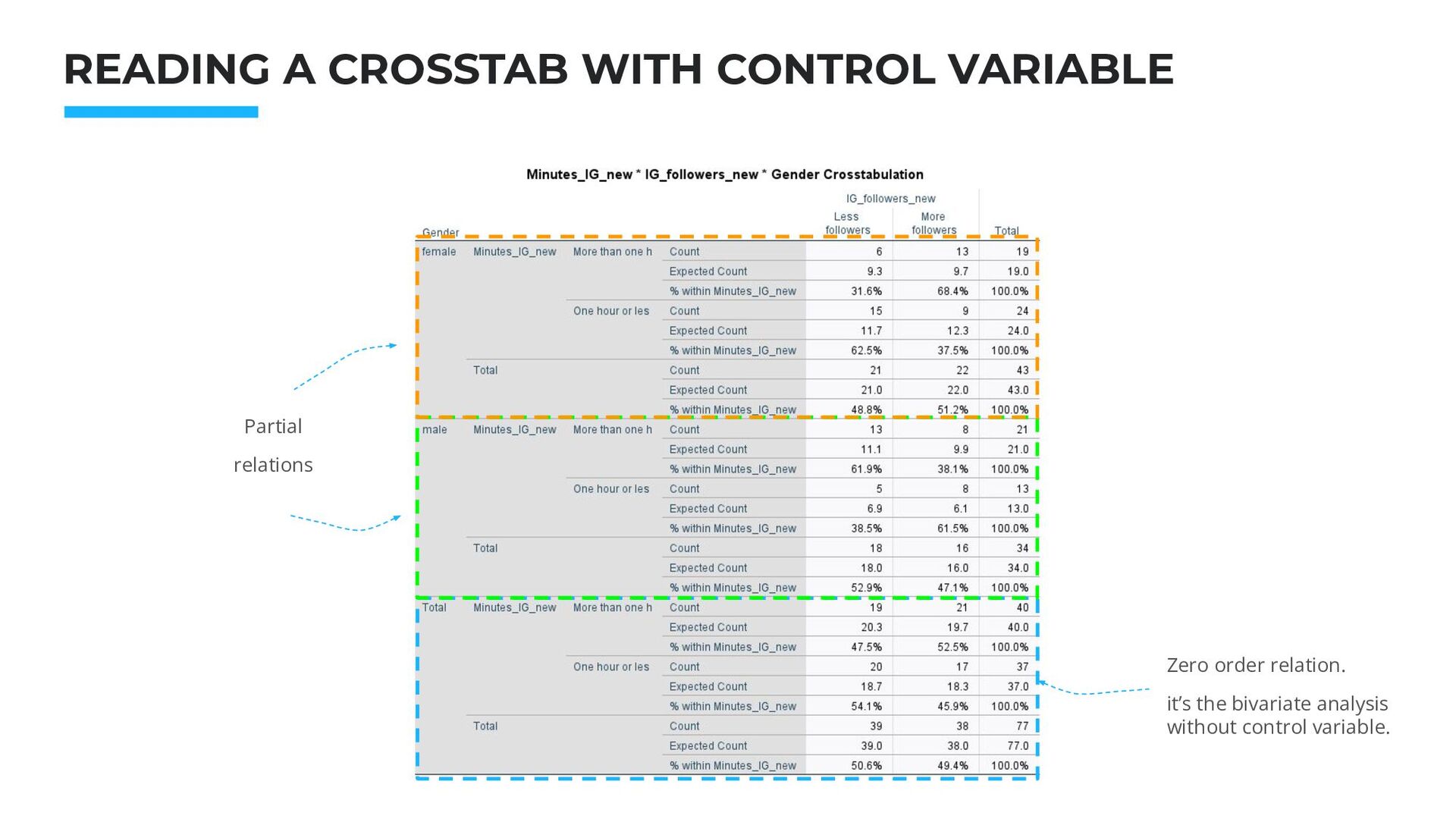
21. Photo: Startup Weekend Hackathon. Nov.2014 ADDING A CONTROL VARIABLE What happens when we add a control variable? Let’s try to add “Gender” as a control variable. To do so, go to Analyze > Descriptive statistics > Crosstab Independent variable in the Rows Dependent variable in the Columns Control variable in the Layer
22. Photo: Startup Weekend Hackathon. Nov.2014 READING A CROSSTAB WITH CONTROL VARIABLE Zero order relation. it’s the bivariate analysis without control variable.
23. Photo: Startup Weekend Hackathon. Nov.2014 READING A CROSSTAB WITH CONTROL VARIABLE Partial relations Zero order relation. it’s the bivariate analysis without control variable.
24. Photo: Startup Weekend Hackathon. Nov.2014 READING A CROSSTAB WITH CONTROL VARIABLE Partial relations Zero order relation. No significant relation between time on instagram and number of followers
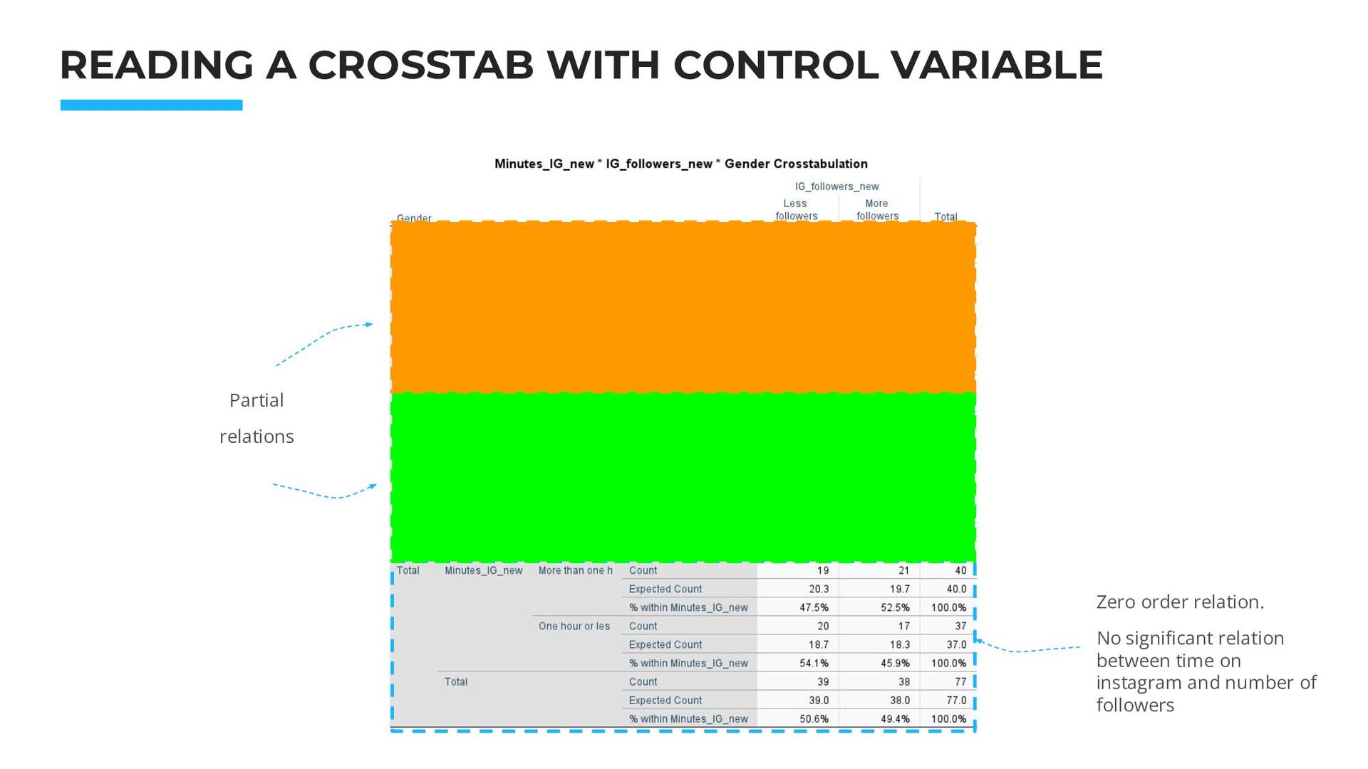
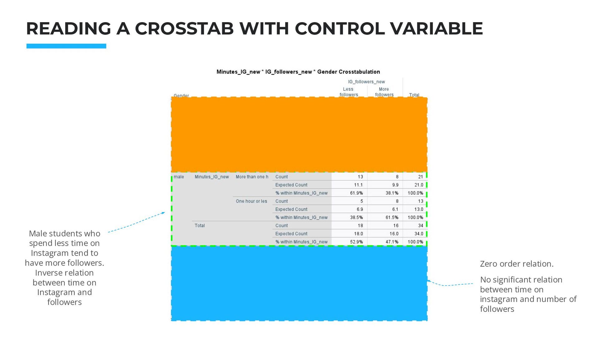
25. Photo: Startup Weekend Hackathon. Nov.2014 READING A CROSSTAB WITH CONTROL VARIABLE Male students who spend less time on Instagram tend to have more followers. Inverse relation between time on Instagram and followers Zero order relation. No significant relation between time on instagram and number of followers
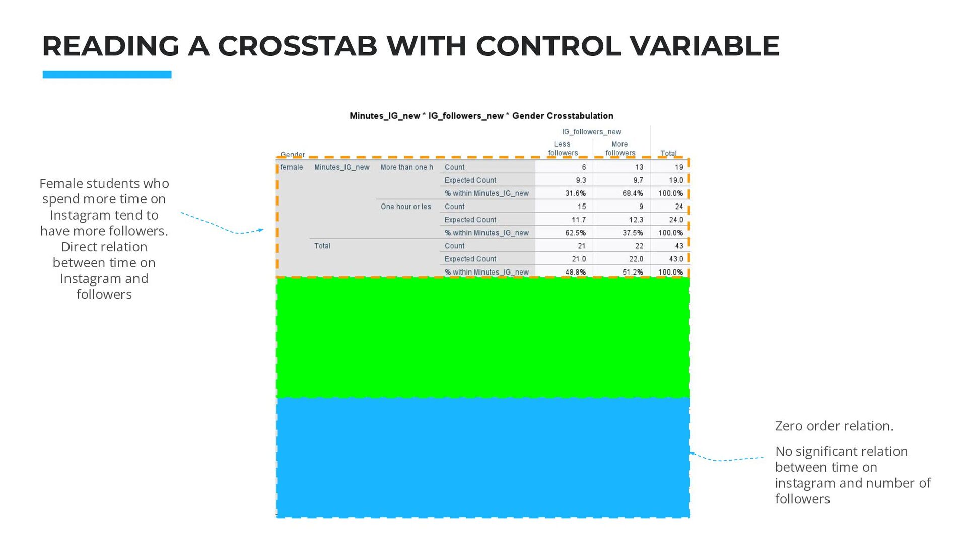
26. Photo: Startup Weekend Hackathon. Nov.2014 READING A CROSSTAB WITH CONTROL VARIABLE Zero order relation. No significant relation between time on instagram and number of followers Female students who spend more time on Instagram tend to have more followers. Direct relation between time on Instagram and followers
27. Photo: Startup Weekend Hackathon. Nov.2014 INTERPRETING THE RESULTS The control variable revealed inverse and direct significant relations in the partials, while the zero order relation confirmed the null hypothesis (no relation between time on Instagram and number of followers). Therefore, we can conclude that the Gender is a suppressor variable (see Prof.Al-Rawi Week 8 videos for the kind of relations between independent, dependent and control variables).
28. Photo: Startup Weekend Hackathon. Nov.2014 INTERPRETING THE RESULTS In general, begin by commenting the zero order relation. Is there a significant (more than 10%) relation? Is it direct or inverse? Then analyze each partial. 1. Is the relation’s direction (direct or inverse) in each partial the same as the zero sum relation? 2. Is it more or less intense than the zero sum relation? (meaning, is the difference in % greater or lower). 3. Is it significant? (more than than 10%) Lastly, try to map the variables using the models described in Prof.Al-Rawi Week 8 lecture? (specification, interpretation, explanation, replication, suppressor variable, distorter variable).
29. Photo: Startup Weekend Hackathon. Nov.2014 EXERCISE Repeat the same crosstab done in class: independent variable: time on Instagram. Dependent variable: number of followers. Instead of using Gender as a control variable, try to use Canadian_birth. Does the result change? Upload the crosstab with the control variable and comment on the partial relations. Upload a screenshot of the crosstab on Canvas alongside a one sentence comment about the relation (or lack thereof) between the two variables.
30. THANK YOU Alberto Lusoli alusoli@sfu.ca Office hour: Thursday, 12.30pm - 1.20pm (please book an appointment in advance via email).