CMNS201 - Lab 8. Assignment 3

Transcript

1. Assignment 3 SPSS LABORATORY 8
2. Photo: Startup Weekend Hackathon. Nov.2014 LAST WEEK LAB ASSIGNMENT: COMMON PROBLEMS Empty column Variable contains empty/missing values
3. Photo: Startup Weekend Hackathon. Nov.2014 LAST WEEK LAB ASSIGNMENT: COMMON PROBLEMS Filtered out all values due to errors in the Select Cases formula
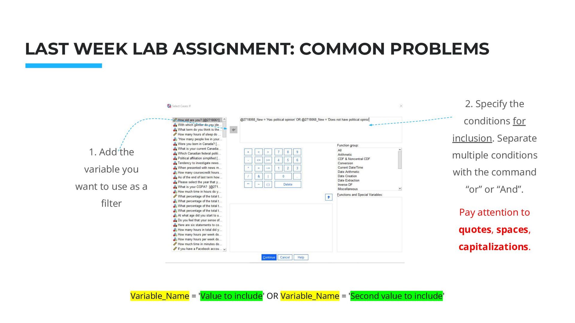
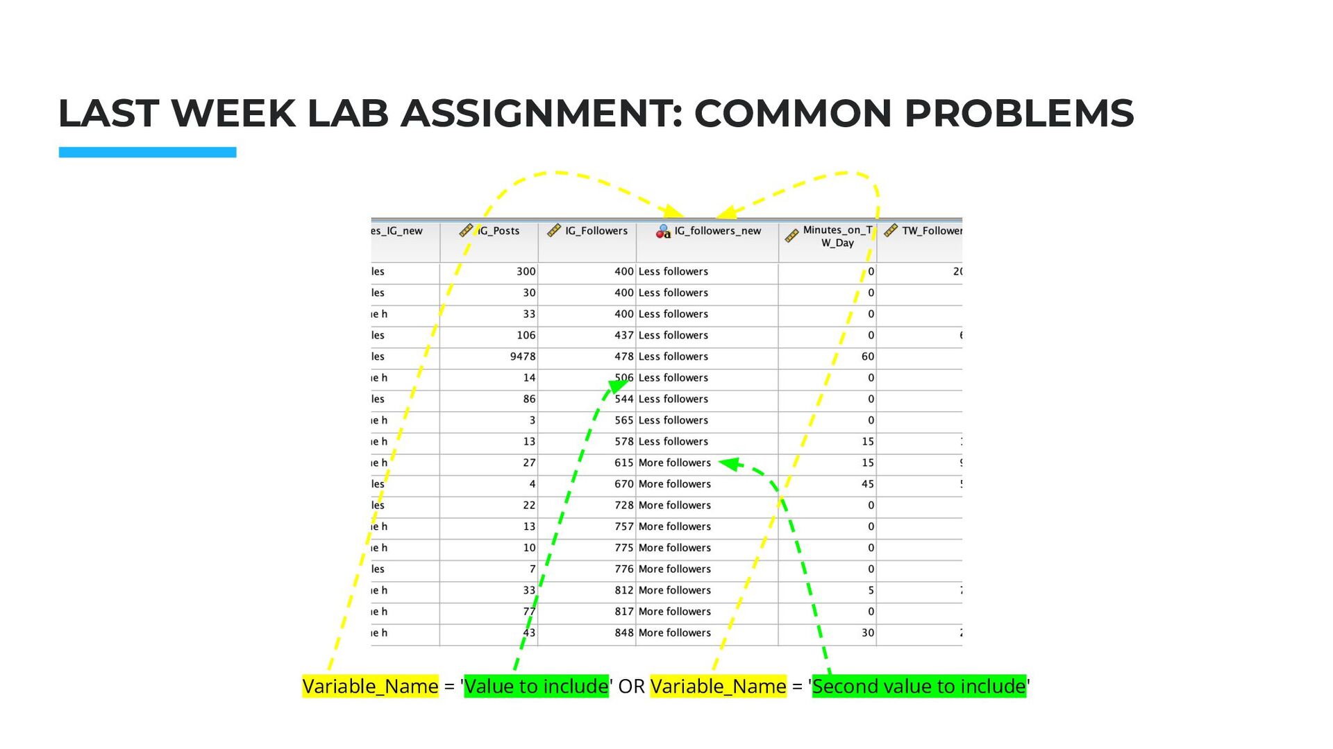
4. Photo: Startup Weekend Hackathon. Nov.2014 LAST WEEK LAB ASSIGNMENT: COMMON PROBLEMS 1. Add the variable you want to use as a filter 2. Specify the conditions for inclusion. Separate multiple conditions with the command “or” or “And”. Pay attention to quotes, spaces, capitalizations. Variable_Name = 'Value to include' OR Variable_Name = 'Second value to include'
5. Photo: Startup Weekend Hackathon. Nov.2014 LAST WEEK LAB ASSIGNMENT: COMMON PROBLEMS Variable_Name = 'Value to include' OR Variable_Name = 'Second value to include'
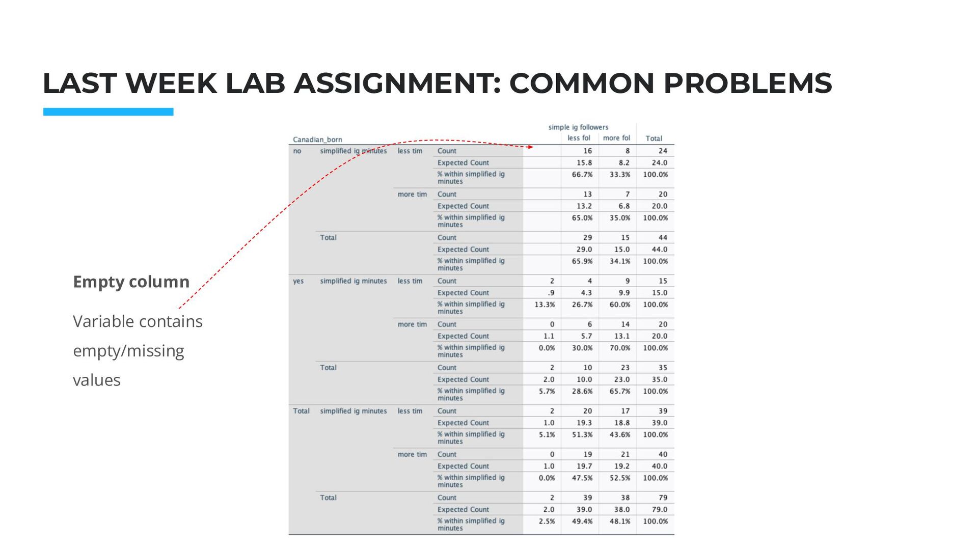
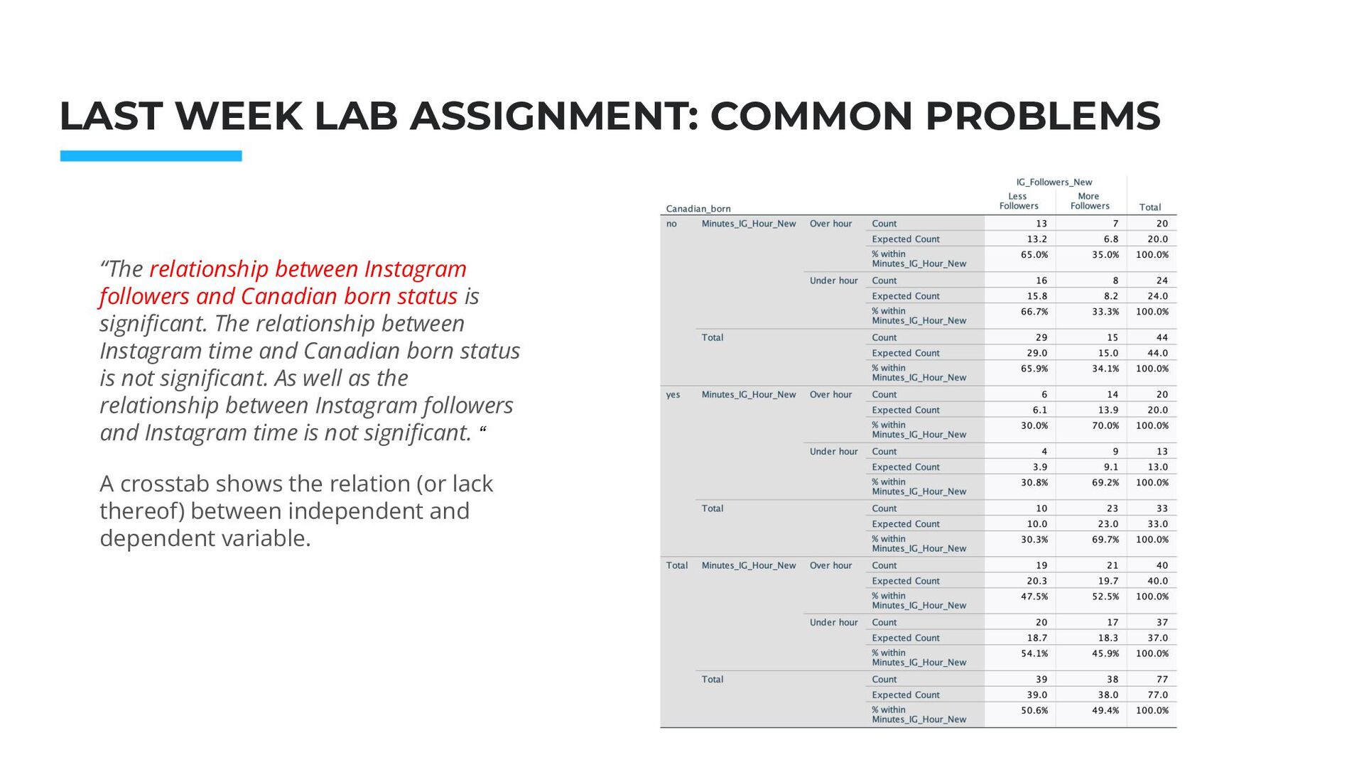
6. Photo: Startup Weekend Hackathon. Nov.2014 LAST WEEK LAB ASSIGNMENT: COMMON PROBLEMS “The relationship between Instagram followers and Canadian born status is significant. The relationship between Instagram time and Canadian born status is not significant. As well as the relationship between Instagram followers and Instagram time is not significant. “ A crosstab shows the relation (or lack thereof) between independent and dependent variable.
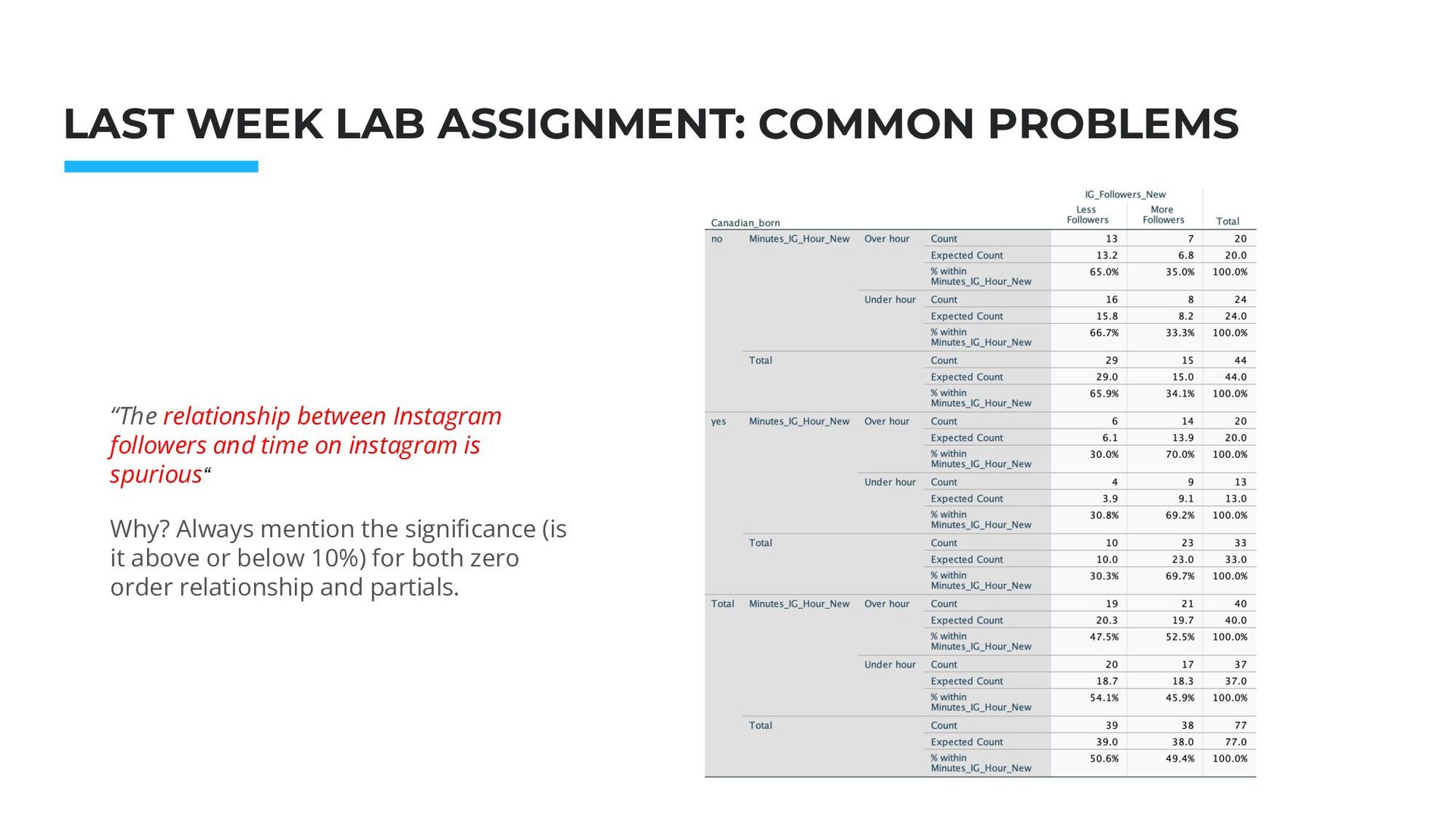
7. Photo: Startup Weekend Hackathon. Nov.2014 LAST WEEK LAB ASSIGNMENT: COMMON PROBLEMS “The relationship between Instagram followers and time on instagram is spurious“ Why? Always mention the significance (is it above or below 10%) for both zero order relationship and partials.
8. 1. Introduction 2. Univariate Statistics 3. Bivariate Statistics A 4. Multivariate Statistics B 5. Sampling 6. Critique of the survey 7. Future research ASSIGNMENT 3 STRUCTURE
9. 1. CHOOSING VARIABLES
10. Photo: Startup Weekend Hackathon. Nov.2014 AS USUAL, LET’S BEGIN WITH A HYPOTHESIS Hypothesis: People who have a political affiliation will tend to read news more carefully and to investigate more to understand is something they read online is a legit news or misinformation. On the contrary, people without a political affiliation will be less likely to spend time investigating news sources. Control variable: We will control the relation between political affiliation and tendency to investigate news sources through a variable measuring how much of an impact social media have on media consumption. Null hypothesis: there is no relationship between political affiliation and tendency to investigate news sources.
11. Photo: Startup Weekend Hackathon. Nov.2014 STEP 1: CHOOSE YOUR VARIABLES • Independent variable: ◦ @2718068 (Which Canadian federal political party do you think best represents your personal political orientation?) • Dependent variable: ◦ @2864544 (When presented with news media on social media platforms, how often do you further analyze or investigate the news media in question in order to discern misinformation?) • Control variable: ◦ @2864568 (How much of an impact does social media have on your media consumption?)
12. 2. RECODING VARIABLES
13. Photo: Startup Weekend Hackathon. Nov.2014 STEP 2: RECODING YOUR VARIABLES All variables (independent, dependent and control) must be binary. Which means, must include only 2 values (for example, younger, older, more followers, less followers, high GPA, low GPA,etc.). Therefore, it is very likely you will have to recode your variables in order to convert them from their original format to a binary form (for how to recode variables, see week 3 lab).
14. Photo: Startup Weekend Hackathon. Nov.2014 Right click on the independent variable name and select Descriptive Statistics. STEP 2: RECODING YOUR VARIABLES 2.2 RECODING THE INDEPENDENT VARIABLE
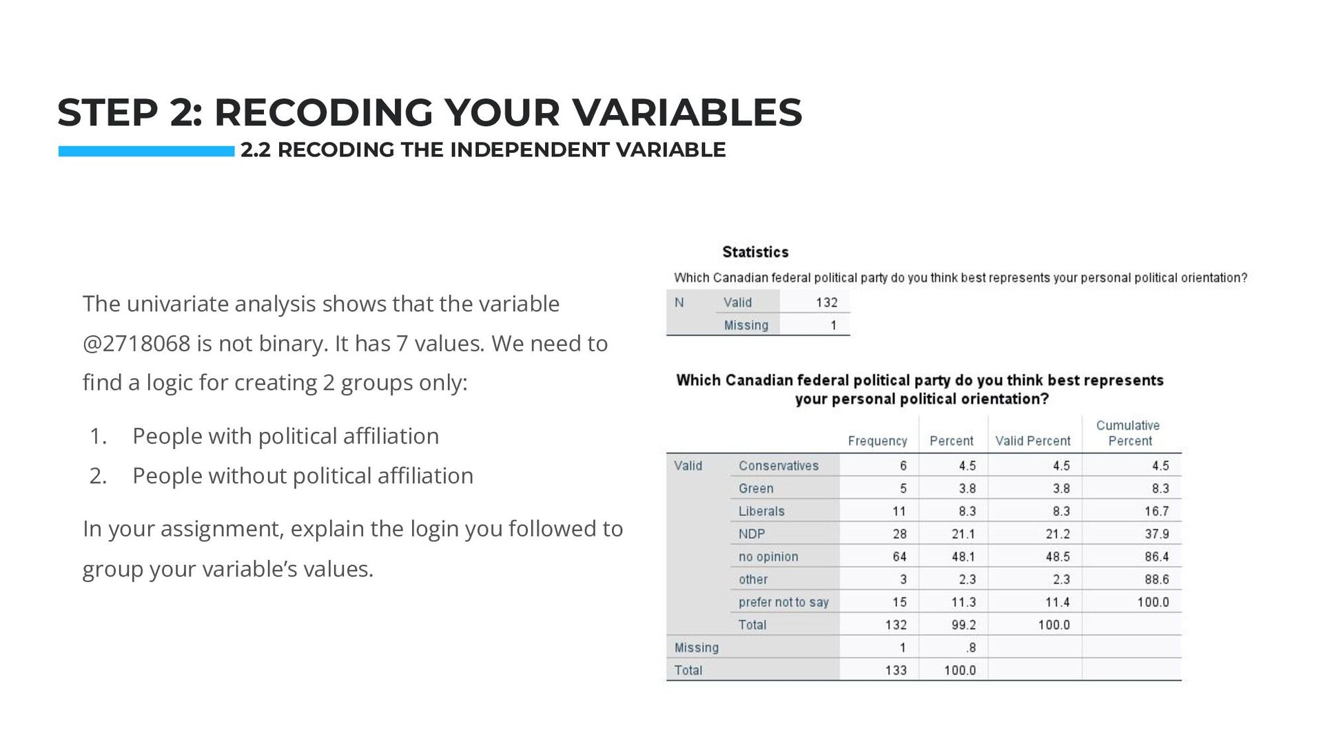
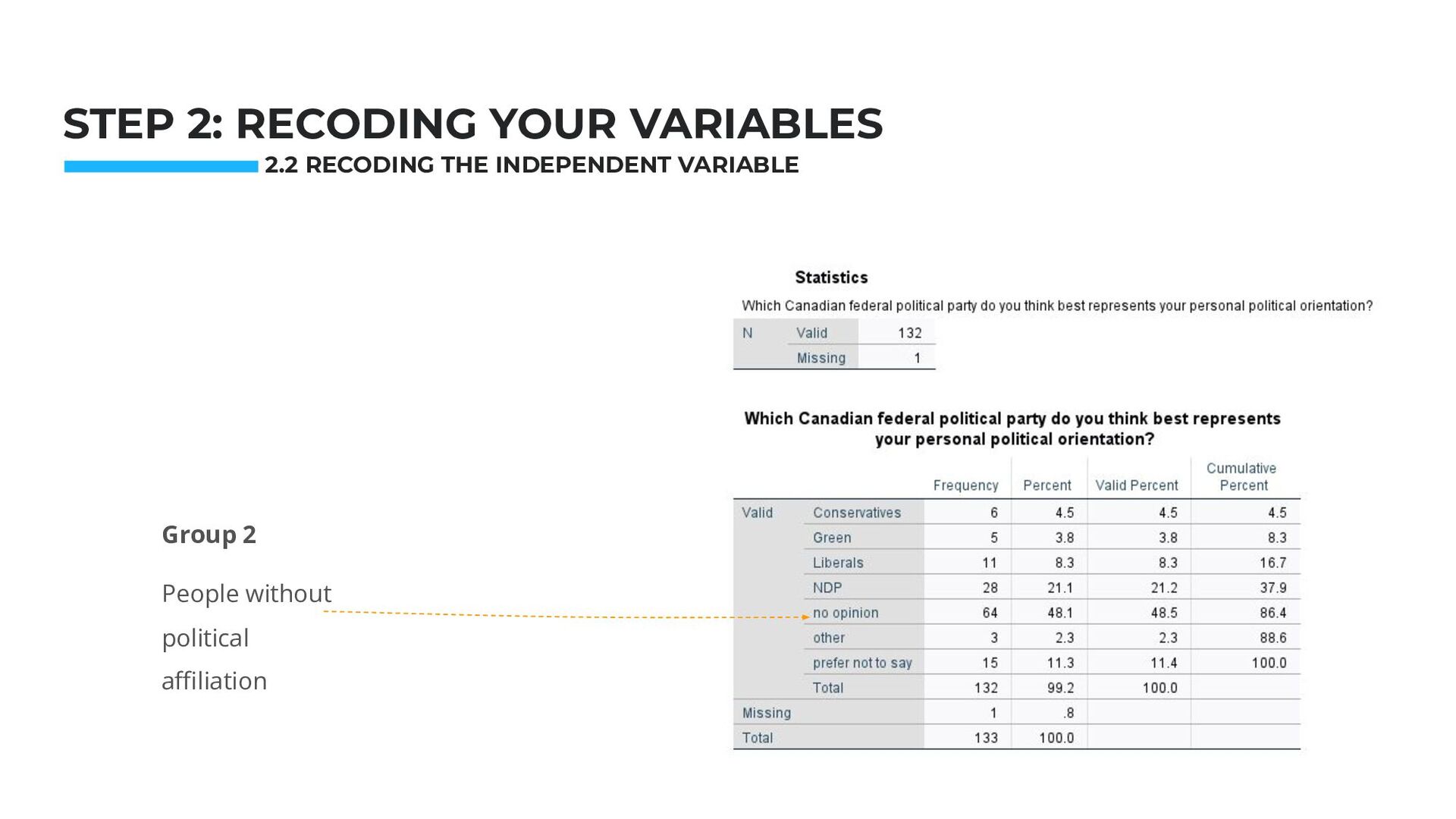
15. The univariate analysis shows that the variable @2718068 is not binary. It has 7 values. We need to find a logic for creating 2 groups only: 1. People with political affiliation 2. People without political affiliation In your assignment, explain the login you followed to group your variable’s values. Photo: Startup Weekend Hackathon. Nov.2014 STEP 2: RECODING YOUR VARIABLES 2.2 RECODING THE INDEPENDENT VARIABLE
16. Photo: Startup Weekend Hackathon. Nov.2014 STEP 2: RECODING YOUR VARIABLES Group 1 People with political affiliation 2.2 RECODING THE INDEPENDENT VARIABLE
17. Photo: Startup Weekend Hackathon. Nov.2014 STEP 2: RECODING YOUR VARIABLES Group 2 People without political affiliation 2.2 RECODING THE INDEPENDENT VARIABLE
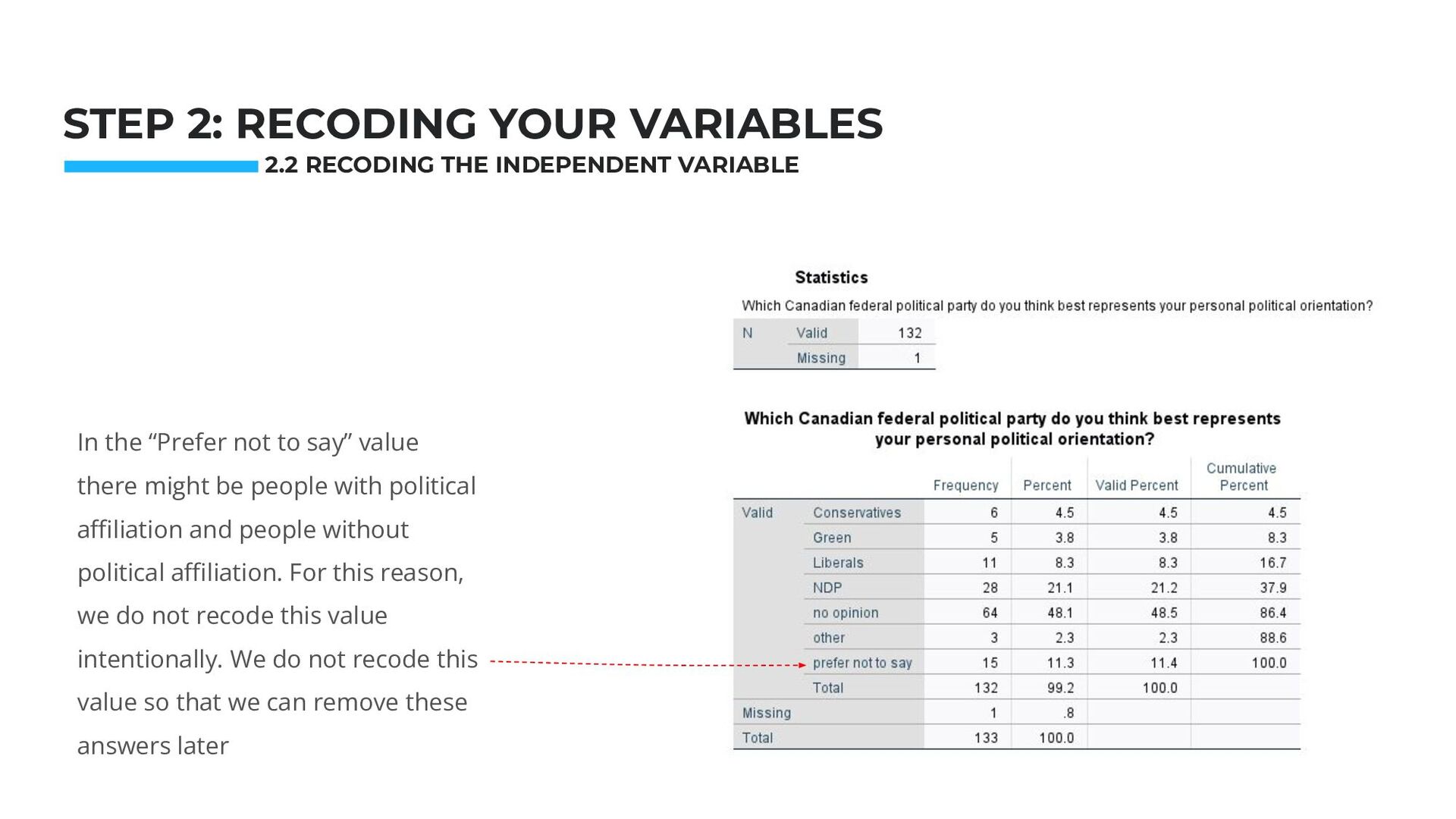
18. Photo: Startup Weekend Hackathon. Nov.2014 STEP 2: RECODING YOUR VARIABLES In the “Prefer not to say” value there might be people with political affiliation and people without political affiliation. For this reason, we do not recode this value intentionally. We do not recode this value so that we can remove these answers later 2.2 RECODING THE INDEPENDENT VARIABLE
19. Photo: Startup Weekend Hackathon. Nov.2014 STEP 2: RECODING YOUR VARIABLES 2.2 RECODING THE INDEPENDENT VARIABLE Notice that the “Prefer not to say” is absent from the recoding rules
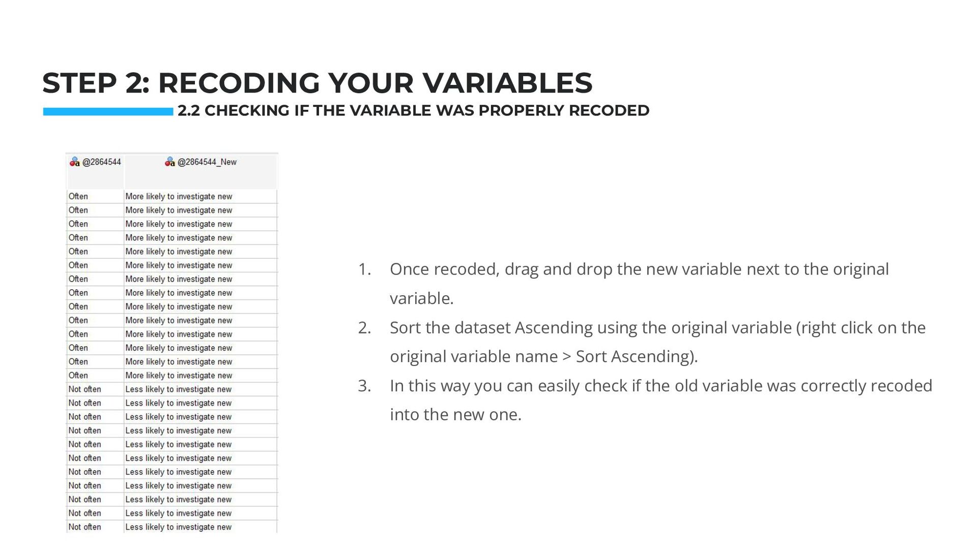
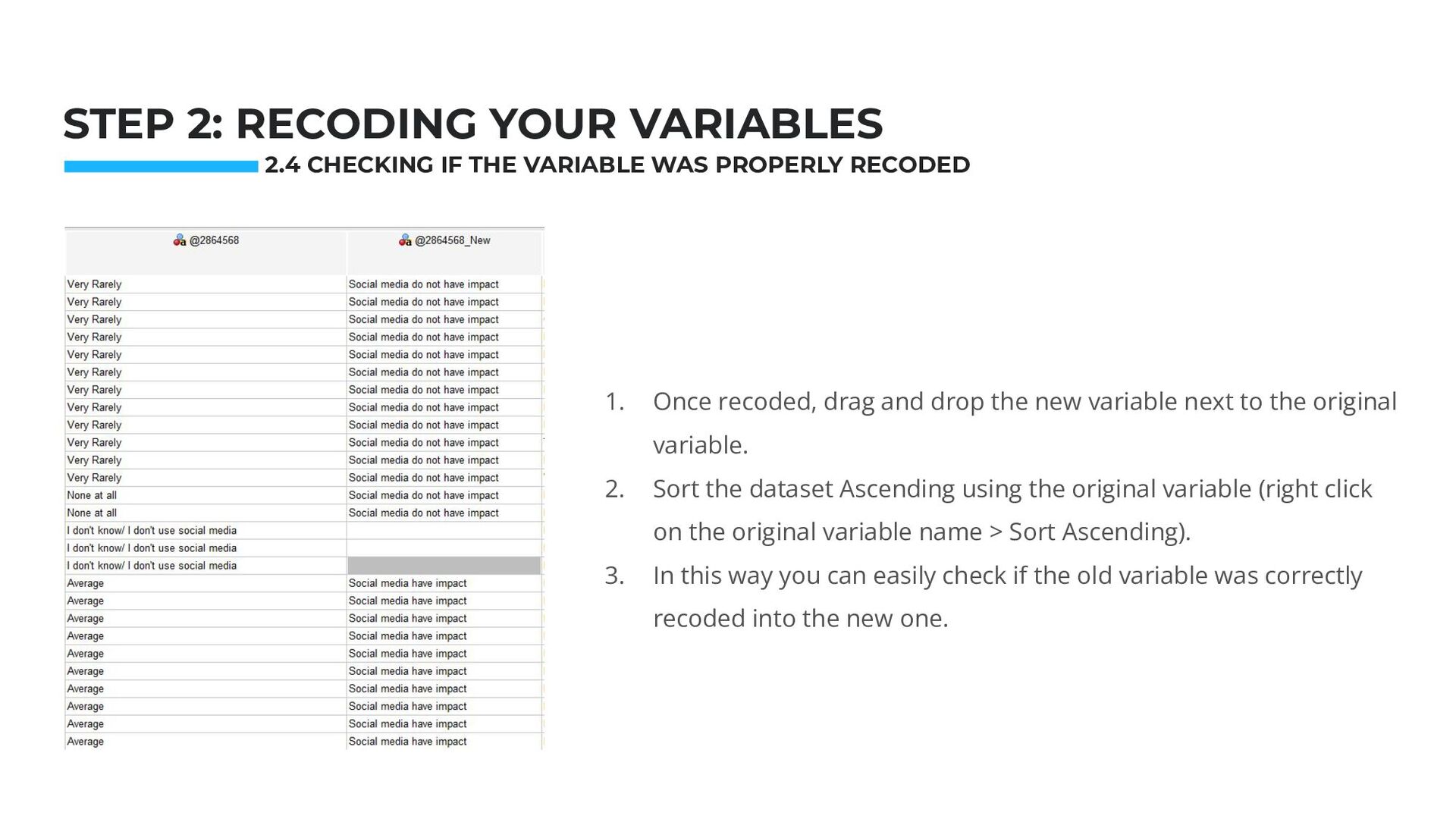
20. 2.2 CHECKING IF THE VARIABLE WAS PROPERLY RECODED Photo: Startup Weekend Hackathon. Nov.2014 STEP 2: RECODING YOUR VARIABLES 1. Once recoded, drag and drop the new variable next to the original variable. 2. Sort the dataset Ascending using the original variable (right click on the original variable name > Sort Ascending). 3. In this way you can easily check if the old variable was correctly recoded into the new one.
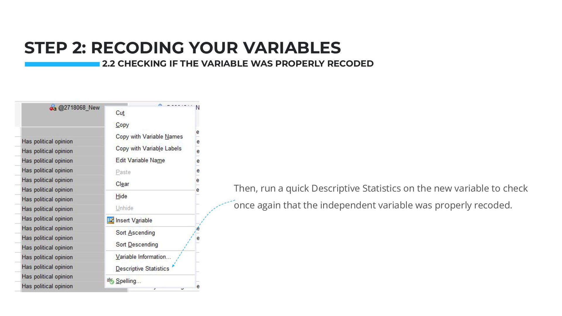
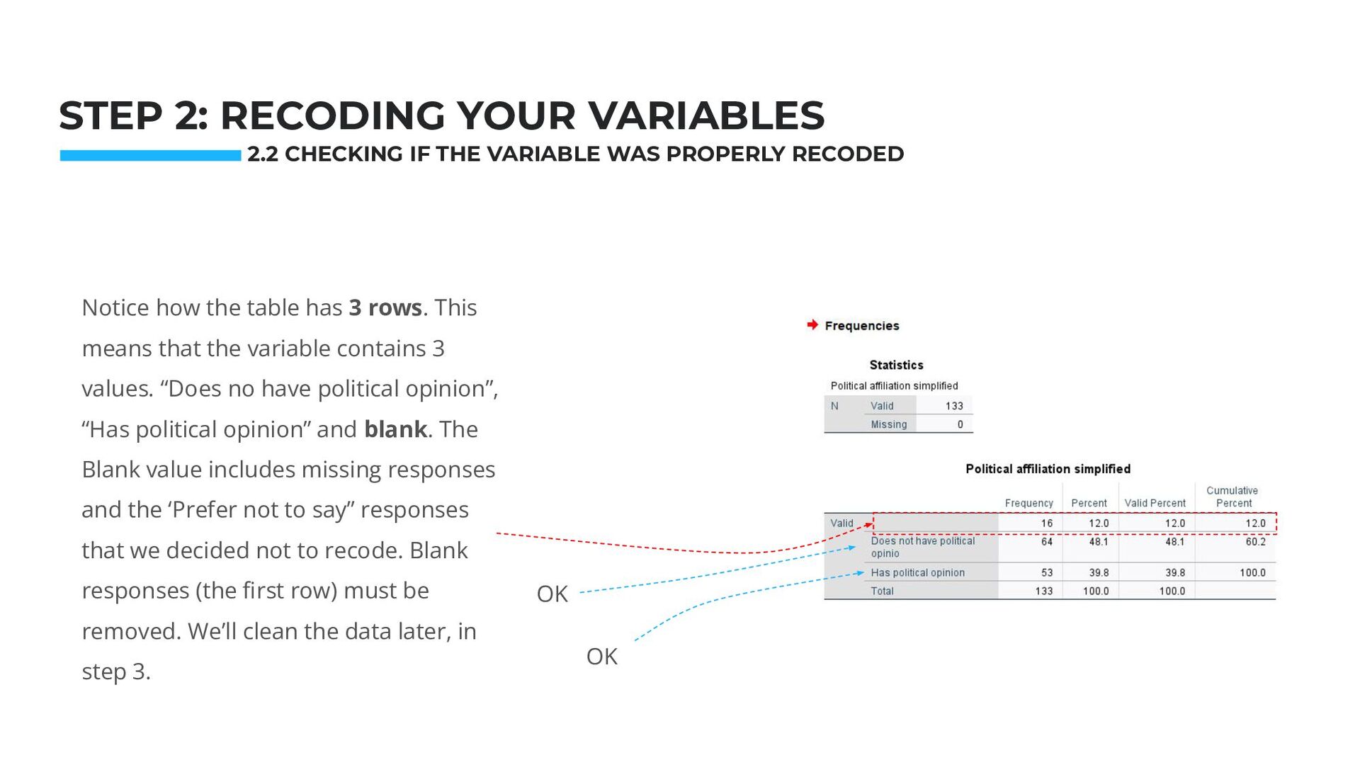
21. Photo: Startup Weekend Hackathon. Nov.2014 STEP 2: RECODING YOUR VARIABLES Then, run a quick Descriptive Statistics on the new variable to check once again that the independent variable was properly recoded. 2.2 CHECKING IF THE VARIABLE WAS PROPERLY RECODED
22. Photo: Startup Weekend Hackathon. Nov.2014 STEP 2: RECODING YOUR VARIABLES OK OK Notice how the table has 3 rows. This means that the variable contains 3 values. “Does no have political opinion”, “Has political opinion” and blank. The Blank value includes missing responses and the ‘Prefer not to say” responses that we decided not to recode. Blank responses (the first row) must be removed. We’ll clean the data later, in step 3. 2.2 CHECKING IF THE VARIABLE WAS PROPERLY RECODED
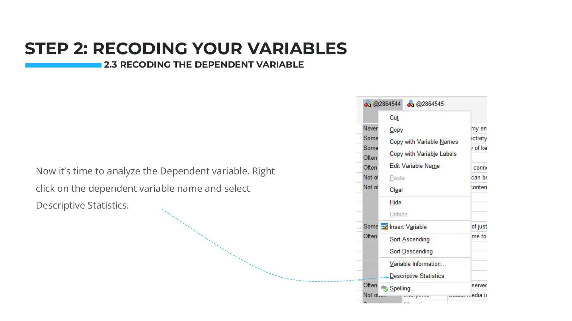
23. Photo: Startup Weekend Hackathon. Nov.2014 Now it’s time to analyze the Dependent variable. Right click on the dependent variable name and select Descriptive Statistics. STEP 2: RECODING YOUR VARIABLES 2.3 RECODING THE DEPENDENT VARIABLE
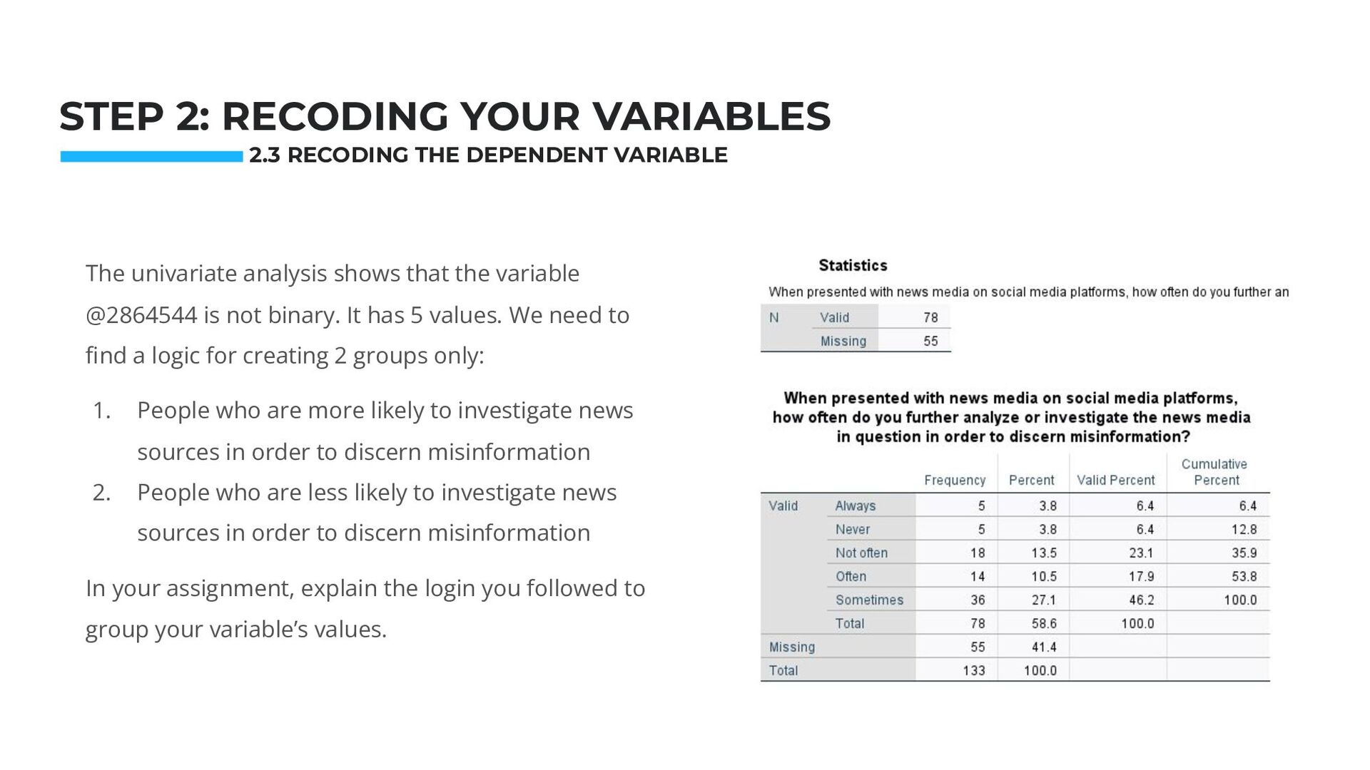
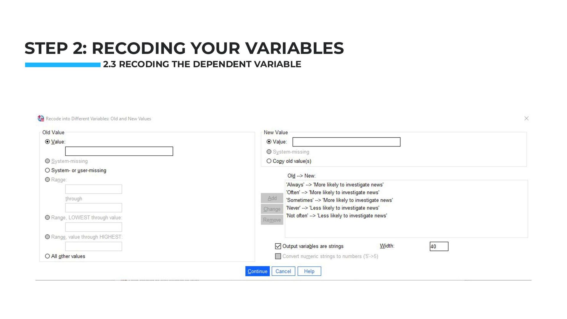
24. Photo: Startup Weekend Hackathon. Nov.2014 STEP 2: RECODING YOUR VARIABLES The univariate analysis shows that the variable @2864544 is not binary. It has 5 values. We need to find a logic for creating 2 groups only: 1. People who are more likely to investigate news sources in order to discern misinformation 2. People who are less likely to investigate news sources in order to discern misinformation In your assignment, explain the login you followed to group your variable’s values. 2.3 RECODING THE DEPENDENT VARIABLE
25. Photo: Startup Weekend Hackathon. Nov.2014 Group 1 People who answered Always, Often or Sometimes will be grouped into the “More likely to investigate news” value of the new recoded variable. STEP 2: RECODING YOUR VARIABLES 2.3 RECODING THE DEPENDENT VARIABLE
26. Photo: Startup Weekend Hackathon. Nov.2014 Group 2 While people who answered Not often or Never will be grouped into the “Less likely to investigate news” value of the new recoded variable. STEP 2: RECODING YOUR VARIABLES 2.3 RECODING THE DEPENDENT VARIABLE
27. Photo: Startup Weekend Hackathon. Nov.2014 STEP 2: RECODING YOUR VARIABLES 2.3 RECODING THE DEPENDENT VARIABLE
28. 2.2 CHECKING IF THE VARIABLE WAS PROPERLY RECODED Photo: Startup Weekend Hackathon. Nov.2014 STEP 2: RECODING YOUR VARIABLES 1. Once recoded, drag and drop the new variable next to the original variable. 2. Sort the dataset Ascending using the original variable (right click on the original variable name > Sort Ascending). 3. In this way you can easily check if the old variable was correctly recoded into the new one.
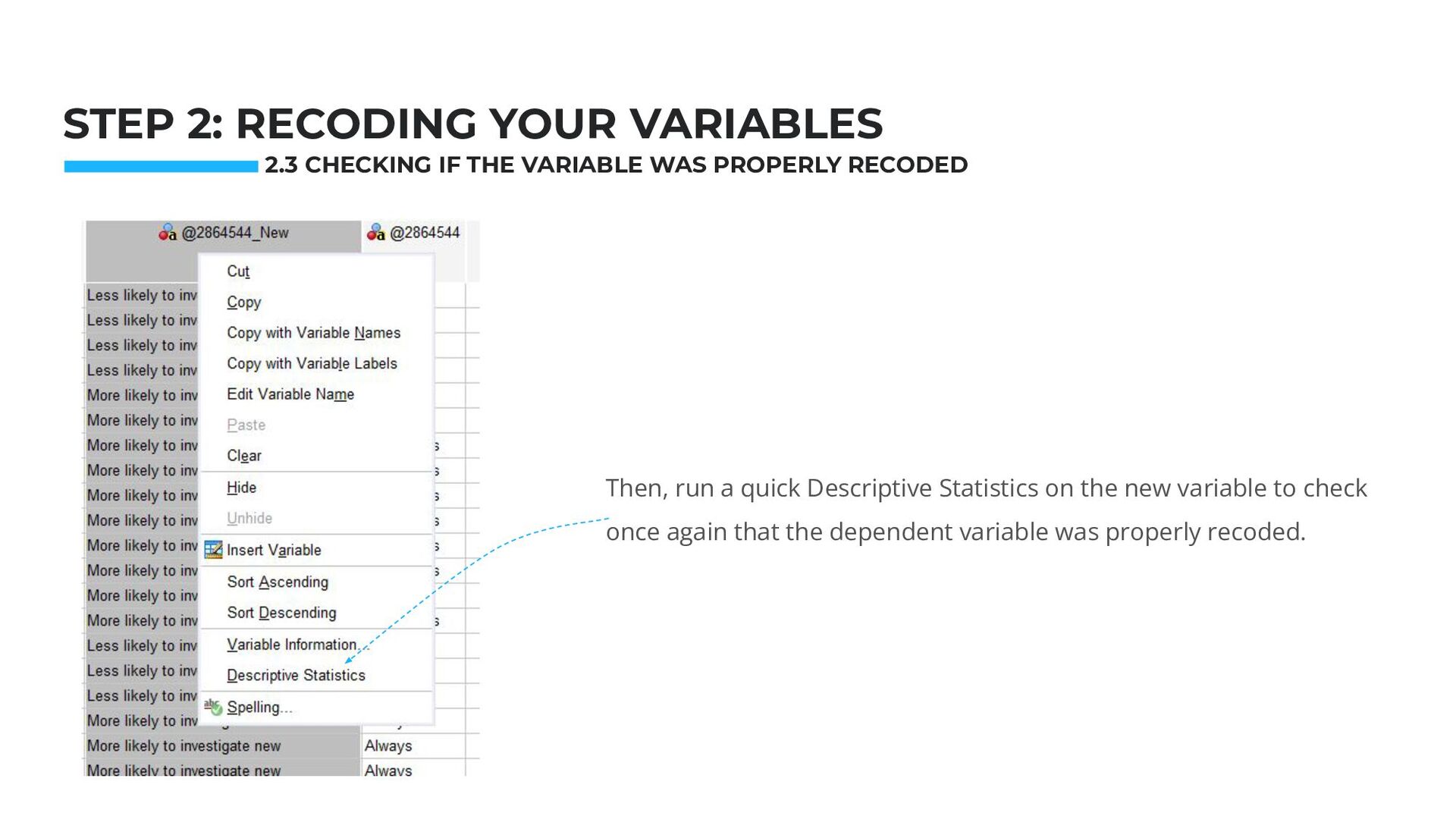
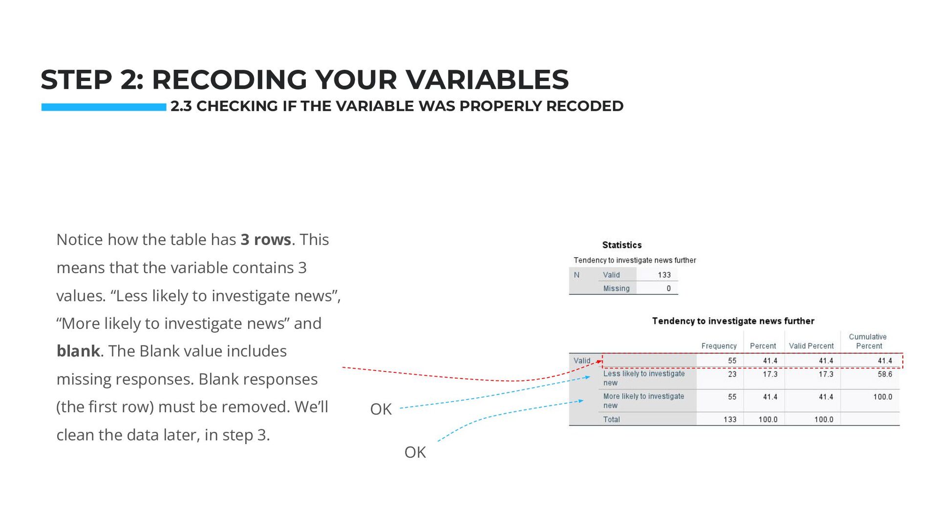
29. Photo: Startup Weekend Hackathon. Nov.2014 STEP 2: RECODING YOUR VARIABLES Then, run a quick Descriptive Statistics on the new variable to check once again that the dependent variable was properly recoded. 2.3 CHECKING IF THE VARIABLE WAS PROPERLY RECODED
30. Notice how the table has 3 rows. This means that the variable contains 3 values. “Less likely to investigate news”, “More likely to investigate news” and blank. The Blank value includes missing responses. Blank responses (the first row) must be removed. We’ll clean the data later, in step 3. Photo: Startup Weekend Hackathon. Nov.2014 STEP 2: RECODING YOUR VARIABLES OK OK 2.3 CHECKING IF THE VARIABLE WAS PROPERLY RECODED
31. Photo: Startup Weekend Hackathon. Nov.2014 Lastly, analyze the Control variable. Right click on the control variable name and select Descriptive Statistics. STEP 2: RECODING YOUR VARIABLES 2.4 RECODING THE CONTROL VARIABLE
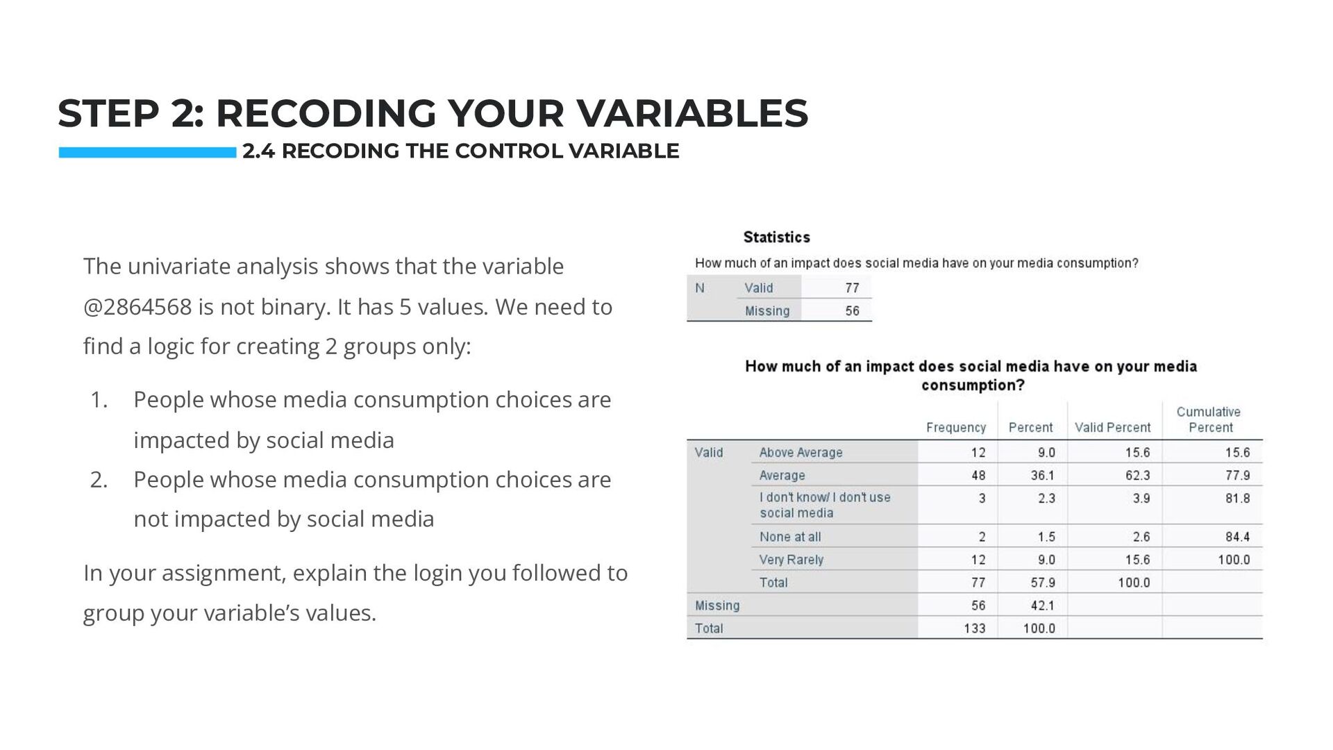
32. Photo: Startup Weekend Hackathon. Nov.2014 The univariate analysis shows that the variable @2864568 is not binary. It has 5 values. We need to find a logic for creating 2 groups only: 1. People whose media consumption choices are impacted by social media 2. People whose media consumption choices are not impacted by social media In your assignment, explain the login you followed to group your variable’s values. STEP 2: RECODING YOUR VARIABLES 2.4 RECODING THE CONTROL VARIABLE
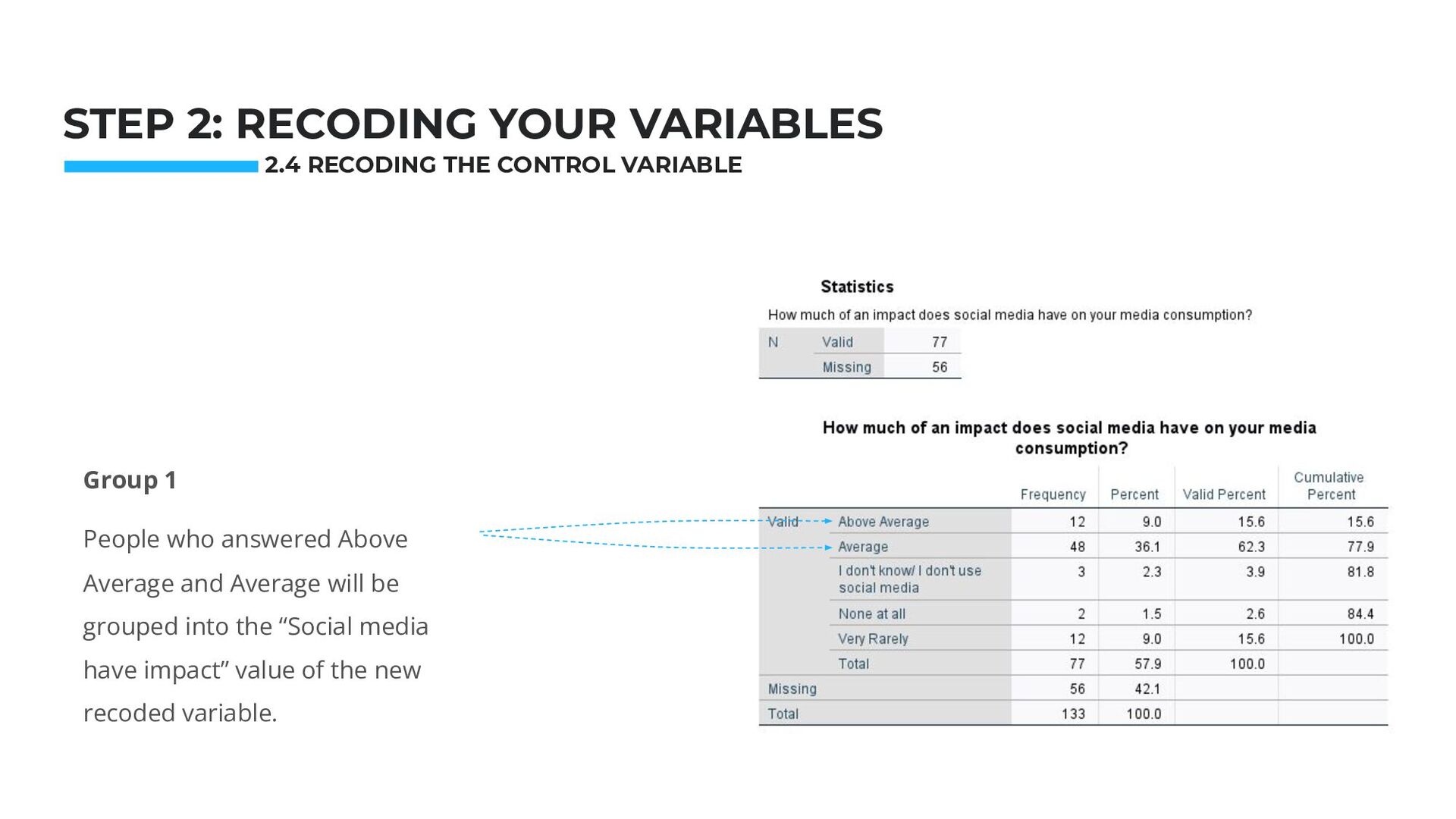
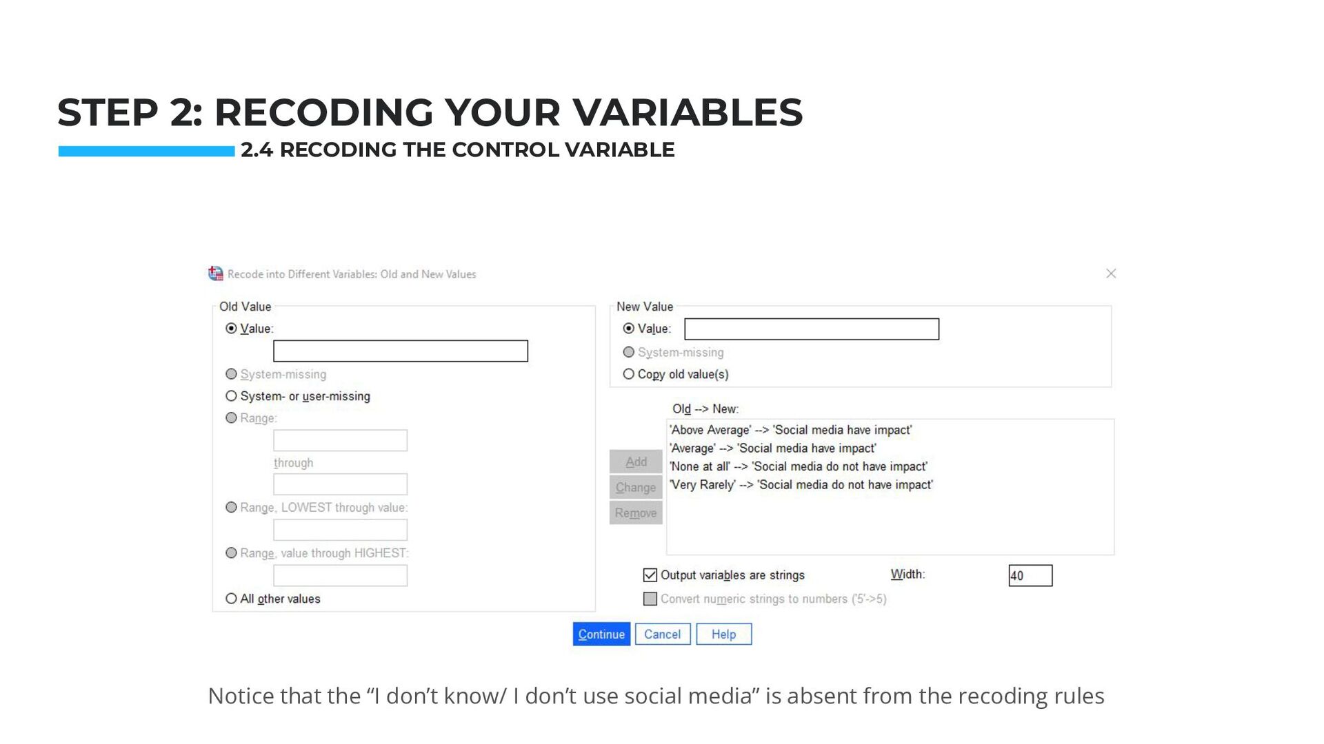
33. Photo: Startup Weekend Hackathon. Nov.2014 Group 1 People who answered Above Average and Average will be grouped into the “Social media have impact” value of the new recoded variable. STEP 2: RECODING YOUR VARIABLES 2.4 RECODING THE CONTROL VARIABLE
34. Photo: Startup Weekend Hackathon. Nov.2014 Group 2 While people who answered Very Rarely and Not at all will be grouped into the “Social media do not have impact” value of the new recoded variable. STEP 2: RECODING YOUR VARIABLES 2.4 RECODING THE CONTROL VARIABLE
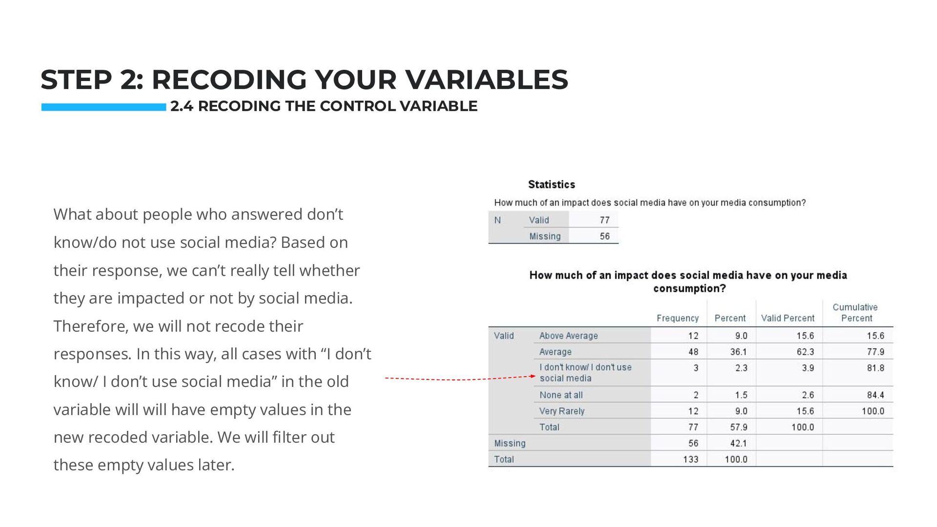
35. What about people who answered don’t know/do not use social media? Based on their response, we can’t really tell whether they are impacted or not by social media. Therefore, we will not recode their responses. In this way, all cases with “I don’t know/ I don’t use social media” in the old variable will will have empty values in the new recoded variable. We will filter out these empty values later. Photo: Startup Weekend Hackathon. Nov.2014 STEP 2: RECODING YOUR VARIABLES 2.4 RECODING THE CONTROL VARIABLE
36. Photo: Startup Weekend Hackathon. Nov.2014 STEP 2: RECODING YOUR VARIABLES 2.4 RECODING THE CONTROL VARIABLE Notice that the “I don’t know/ I don’t use social media” is absent from the recoding rules
37. 2.4 CHECKING IF THE VARIABLE WAS PROPERLY RECODED Photo: Startup Weekend Hackathon. Nov.2014 STEP 2: RECODING YOUR VARIABLES 1. Once recoded, drag and drop the new variable next to the original variable. 2. Sort the dataset Ascending using the original variable (right click on the original variable name > Sort Ascending). 3. In this way you can easily check if the old variable was correctly recoded into the new one.
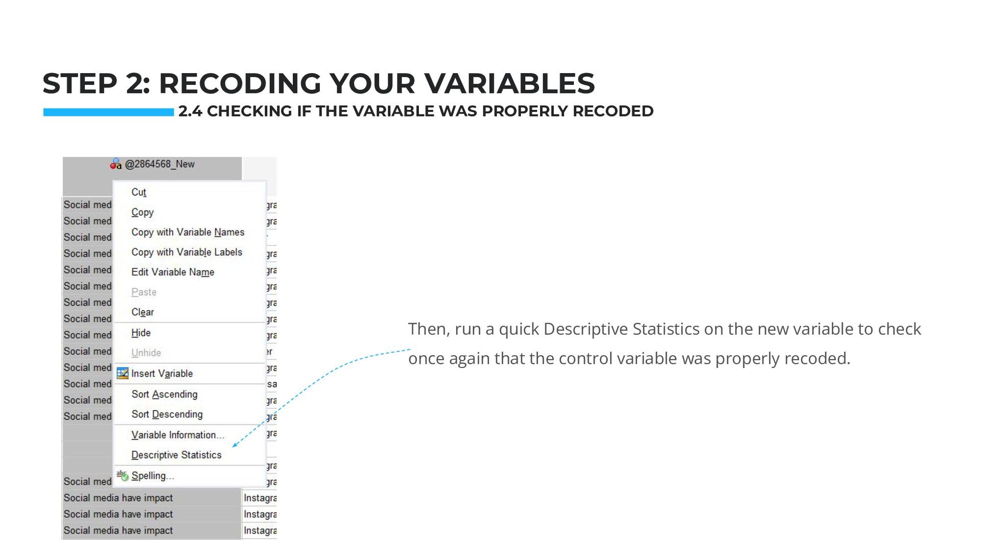
38. Photo: Startup Weekend Hackathon. Nov.2014 STEP 2: RECODING YOUR VARIABLES Then, run a quick Descriptive Statistics on the new variable to check once again that the control variable was properly recoded. 2.4 CHECKING IF THE VARIABLE WAS PROPERLY RECODED
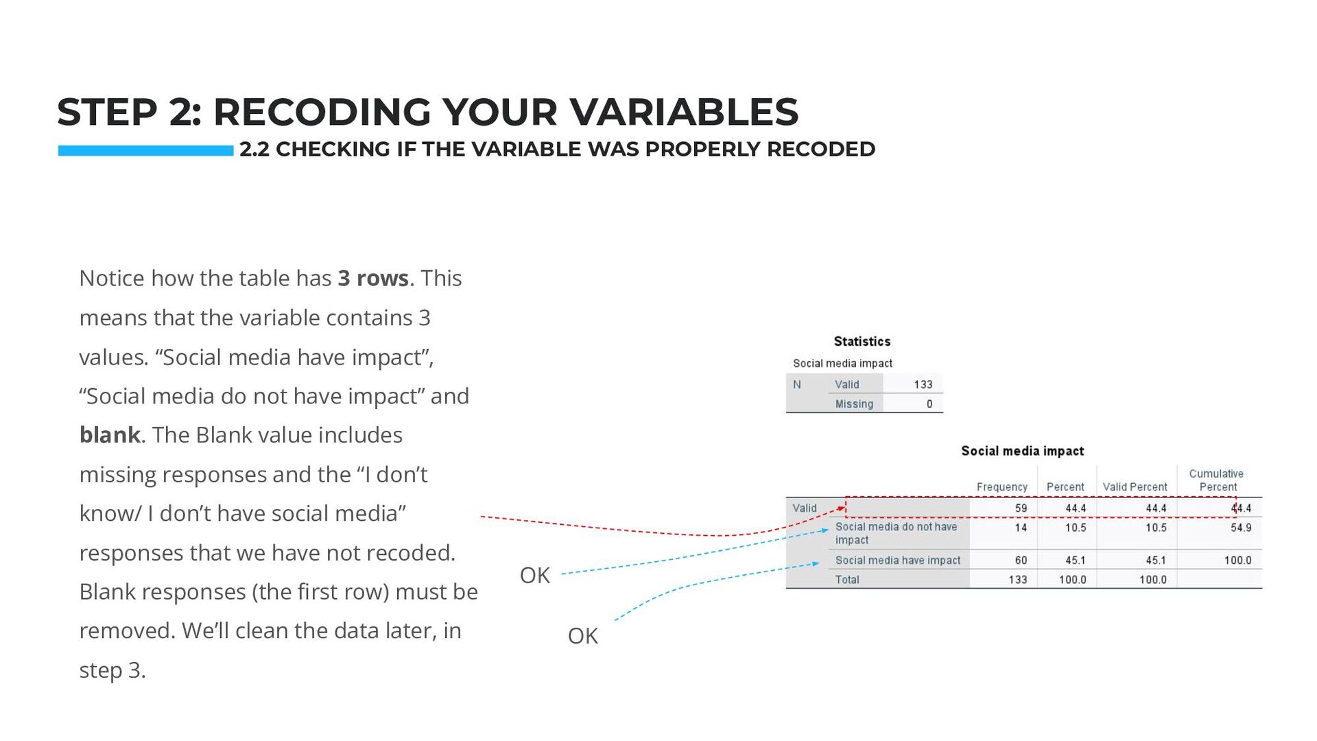
39. Notice how the table has 3 rows. This means that the variable contains 3 values. “Social media have impact”, “Social media do not have impact” and blank. The Blank value includes missing responses and the “I don’t know/ I don’t have social media” responses that we have not recoded. Blank responses (the first row) must be removed. We’ll clean the data later, in step 3. Photo: Startup Weekend Hackathon. Nov.2014 STEP 2: RECODING YOUR VARIABLES OK OK 2.2 CHECKING IF THE VARIABLE WAS PROPERLY RECODED
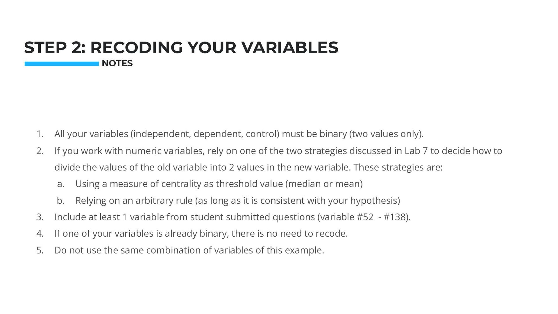
40. 1. All your variables (independent, dependent, control) must be binary (two values only). 2. If you work with numeric variables, rely on one of the two strategies discussed in Lab 7 to decide how to divide the values of the old variable into 2 values in the new variable. These strategies are: a. Using a measure of centrality as threshold value (median or mean) b. Relying on an arbitrary rule (as long as it is consistent with your hypothesis) 3. Include at least 1 variable from student submitted questions (variable #52 - #138). 4. If one of your variables is already binary, there is no need to recode. 5. Do not use the same combination of variables of this example. Photo: Startup Weekend Hackathon. Nov.2014 STEP 2: RECODING YOUR VARIABLES NOTES
41. 3. CLEANING VARIABLES
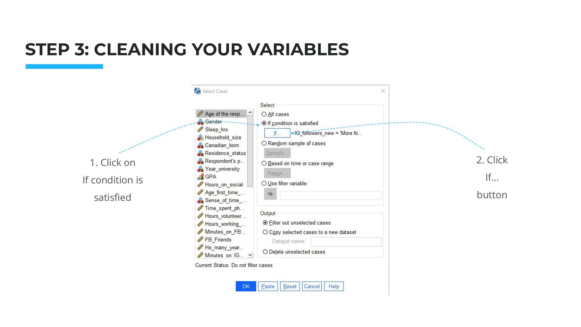
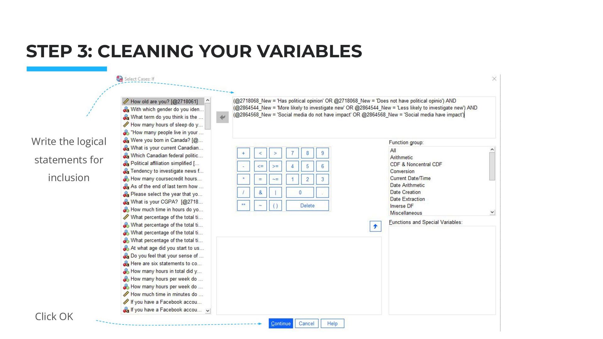
42. Now it’s time to clean the data. As shown in the previous slides, all recoded variables have missing or empty values. We now need to remove empty values from all variables. To do so, click on Data in the top bar and then Select Cases. Photo: Startup Weekend Hackathon. Nov.2014 STEP 3: CLEANING YOUR VARIABLES
43. Photo: Startup Weekend Hackathon. Nov.2014 STEP 3: CLEANING YOUR VARIABLES 1. Click on If condition is satisfied 2. Click If… button
44. In the week 7 Lab, we learned how to remove undesired values from a variable. This is achieved by writing a simple logical statement in the Select cases window. This statement determines which cases SPSS will use in all future calculations. Photo: Startup Weekend Hackathon. Nov.2014 STEP 3: CLEANING YOUR VARIABLES
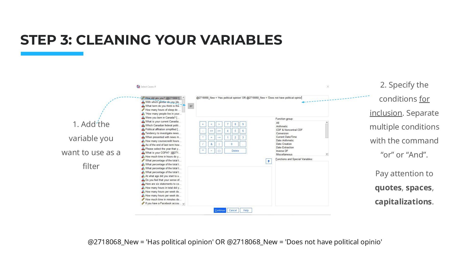
45. Photo: Startup Weekend Hackathon. Nov.2014 STEP 3: CLEANING YOUR VARIABLES 1. Add the variable you want to use as a filter 2. Specify the conditions for inclusion. Separate multiple conditions with the command “or” or “And”. Pay attention to quotes, spaces, capitalizations. @2718068_New = 'Has political opinion' OR @2718068_New = 'Does not have political opinio'
46. The formula showed in the previous slide is appropriate if you have to clean only one variable. However, if more than one of your variables include unwanted values (in other words, if more than one of your variable is not in binary form), then you need to use a more complex formula to remove all unwanted values from all variables at once. The formula is the following: (VARIABLE1 = 'VALUE1' OR VARIABLE1 = 'VALUE2’) AND (VARIABLE2 = 'VALUE1' OR VARIABLE2 = 'VALUE2') AND (VARIABLE3 = 'VALUE1' OR VARIABLE3 = 'VALUE2') Where VARIABLE1 is your independent variable, VARIABLE2 is your dependent variable and VARIABLE3 is your control variable, and VALUE1 and VALUE2 are the respective values you want to include for each variable. Photo: Startup Weekend Hackathon. Nov.2014 STEP 3: CLEANING YOUR VARIABLES
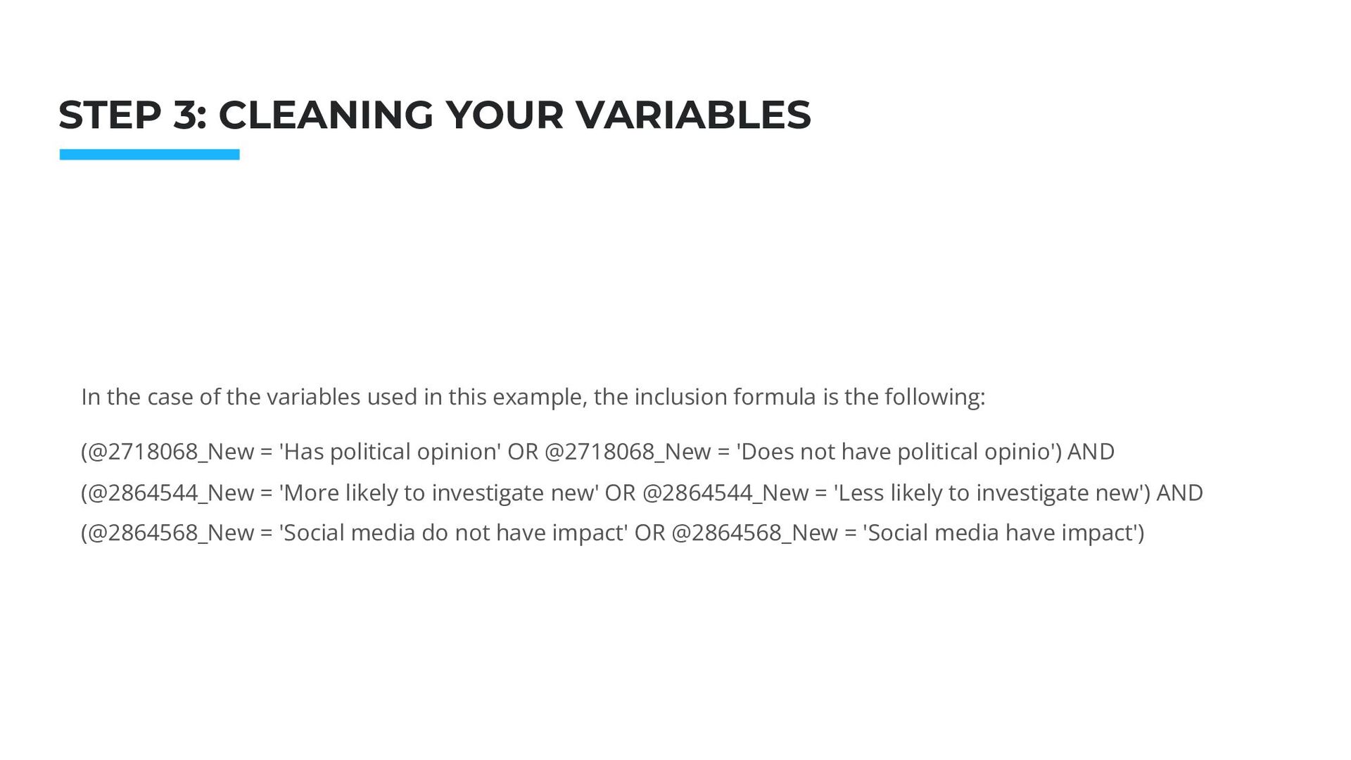
47. In the case of the variables used in this example, the inclusion formula is the following: (@2718068_New = 'Has political opinion' OR @2718068_New = 'Does not have political opinio') AND (@2864544_New = 'More likely to investigate new' OR @2864544_New = 'Less likely to investigate new') AND (@2864568_New = 'Social media do not have impact' OR @2864568_New = 'Social media have impact') Photo: Startup Weekend Hackathon. Nov.2014 STEP 3: CLEANING YOUR VARIABLES
48. Photo: Startup Weekend Hackathon. Nov.2014 STEP 3: CLEANING YOUR VARIABLES Write the logical statements for inclusion Click OK
49. Photo: Startup Weekend Hackathon. Nov.2014 Good job! The most tedious part of Assignment 3 is done. If you successfully recoded and cleaned your variables, you are 80% done. What is left is the fun part: running the analyses. STEP 3: CLEANING YOUR VARIABLES
50. 4. UNIVARIATE ANALYSIS
51. Now, let’s do a univariate analysis for all three variables. Photo: Startup Weekend Hackathon. Nov.2014 STEP 4: UNIVARIATE ANALYSIS
52. Photo: Startup Weekend Hackathon. Nov.2014 STEP 4: UNIVARIATE ANALYSIS
53. Photo: Startup Weekend Hackathon. Nov.2014 STEP 4: UNIVARIATE ANALYSIS Drag and drop your three variables (recoded and cleaned) in the box on the right. Select Statistics and choose the main measures of centrality and dispersion (mean, mode, median, std deviation, range, min and max). Repeat this step for all your 3 variables.
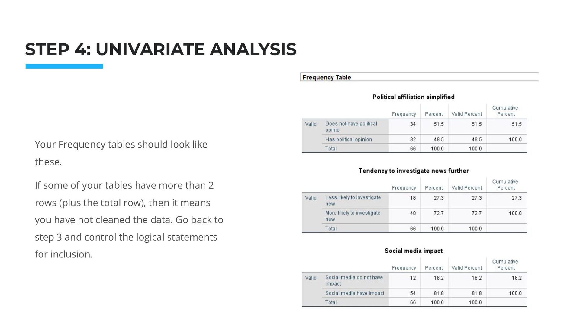
54. Photo: Startup Weekend Hackathon. Nov.2014 STEP 4: UNIVARIATE ANALYSIS Your Frequency tables should look like these. If some of your tables have more than 2 rows (plus the total row), then it means you have not cleaned the data. Go back to step 3 and control the logical statements for inclusion.
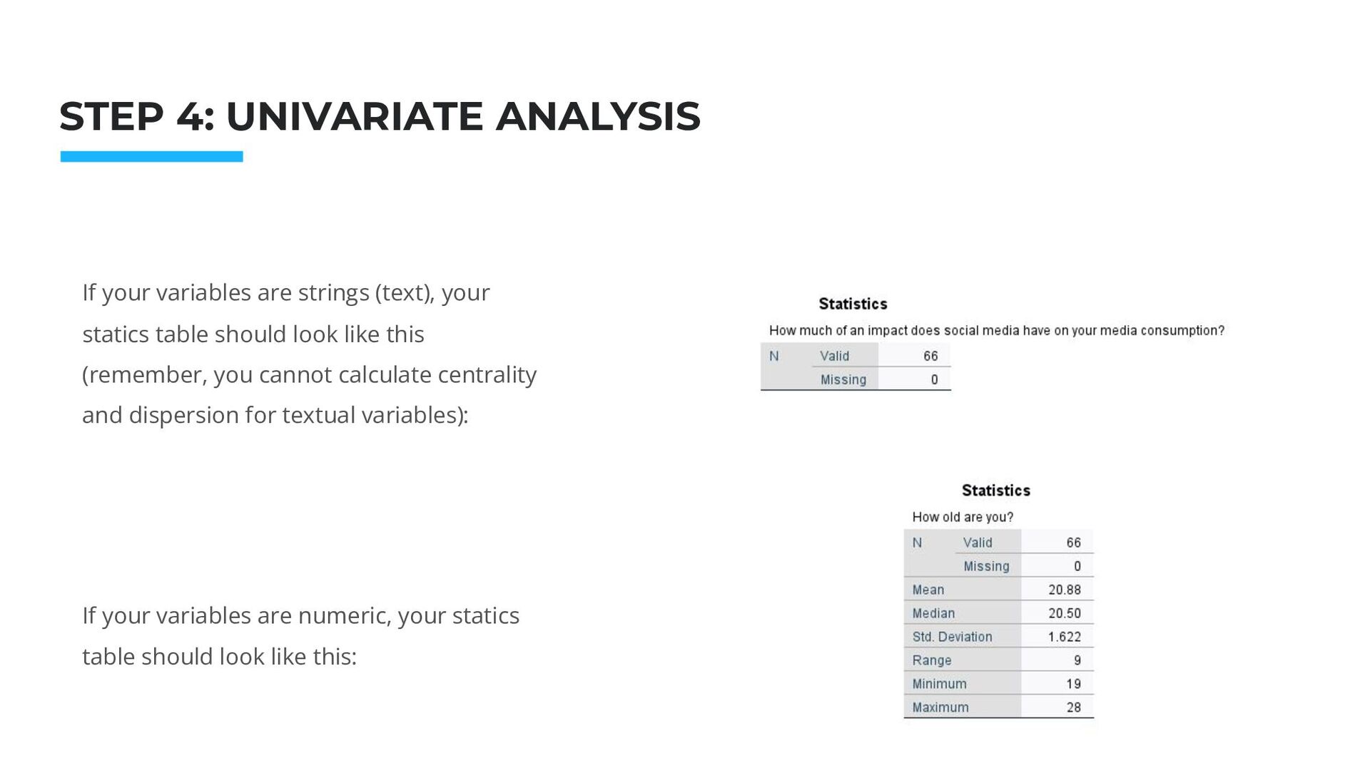
55. Photo: Startup Weekend Hackathon. Nov.2014 STEP 4: UNIVARIATE ANALYSIS If your variables are strings (text), your statics table should look like this (remember, you cannot calculate centrality and dispersion for textual variables): If your variables are numeric, your statics table should look like this:
56. Photo: Startup Weekend Hackathon. Nov.2014 STEP 4: UNIVARIATE ANALYSIS If you really want to go the extra mile, add charts to your analysis. If you do, keep in mind the data visualization best practices described in SPSS Lab 5
57. 4. BIVARIATE ANALYSIS
58. Photo: Startup Weekend Hackathon. Nov.2014 BIVARIATE ANALYSIS
59. Photo: Startup Weekend Hackathon. Nov.2014 SETTING UP YOUR CROSSTAB 1. Independent variable (recoded and cleaned) in the Rows 2. Dependent variable (recoded and cleaned) in the Columns 3. Click Cells
60. Select Observed and Expected counts Photo: Startup Weekend Hackathon. Nov.2014 SETTING UP YOUR CROSSTAB Select Row Click Continue
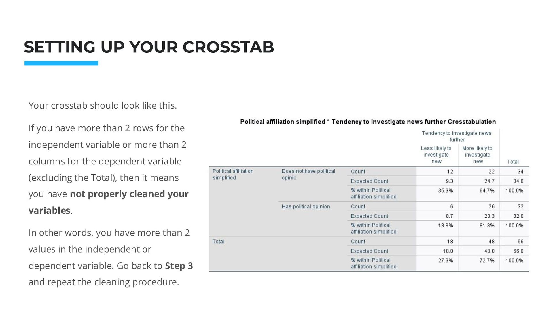
61. Photo: Startup Weekend Hackathon. Nov.2014 SETTING UP YOUR CROSSTAB Your crosstab should look like this. If you have more than 2 rows for the independent variable or more than 2 columns for the dependent variable (excluding the Total), then it means you have not properly cleaned your variables. In other words, you have more than 2 values in the independent or dependent variable. Go back to Step 3 and repeat the cleaning procedure.
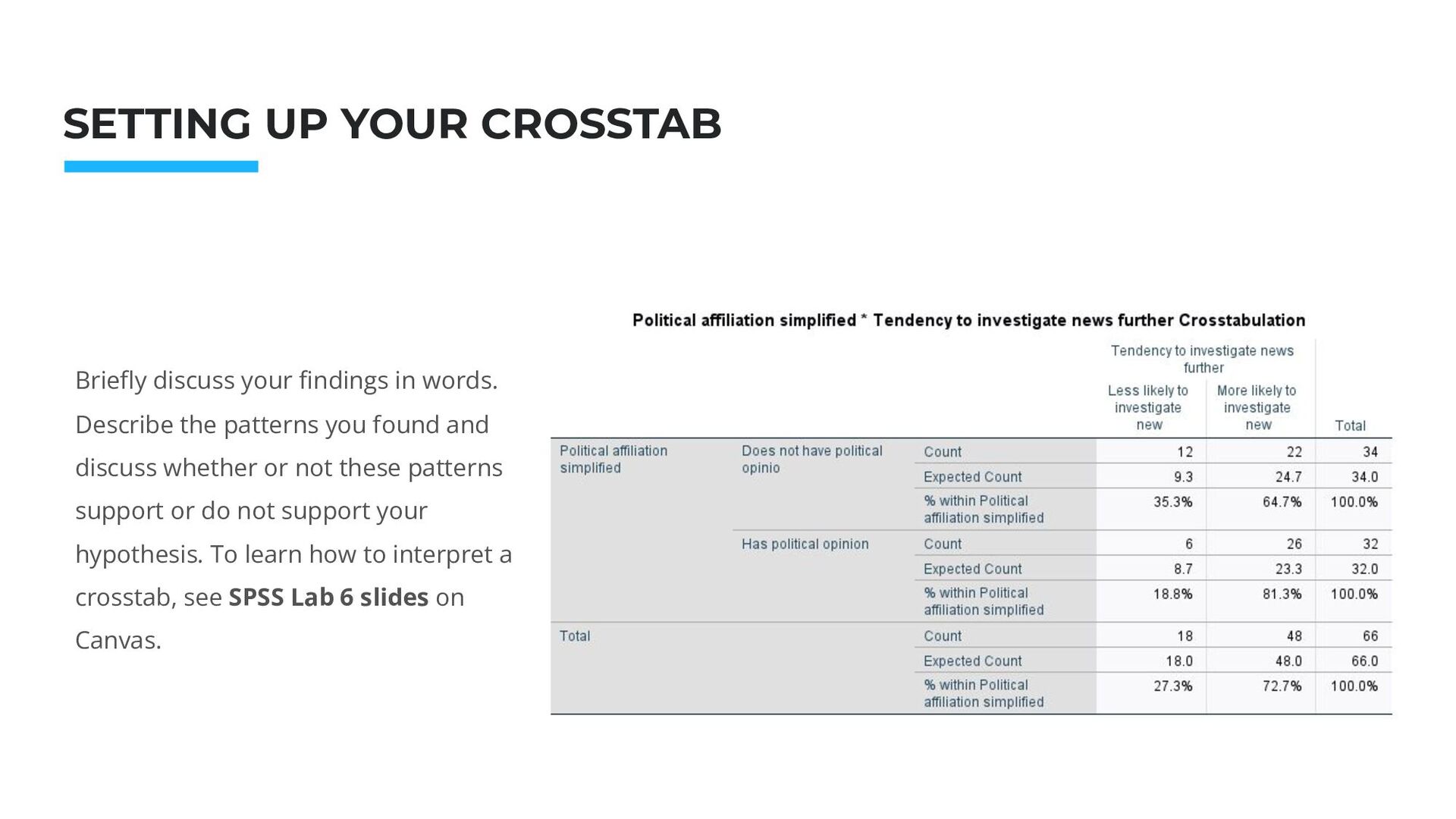
62. Photo: Startup Weekend Hackathon. Nov.2014 SETTING UP YOUR CROSSTAB Briefly discuss your findings in words. Describe the patterns you found and discuss whether or not these patterns support or do not support your hypothesis. To learn how to interpret a crosstab, see SPSS Lab 6 slides on Canvas.
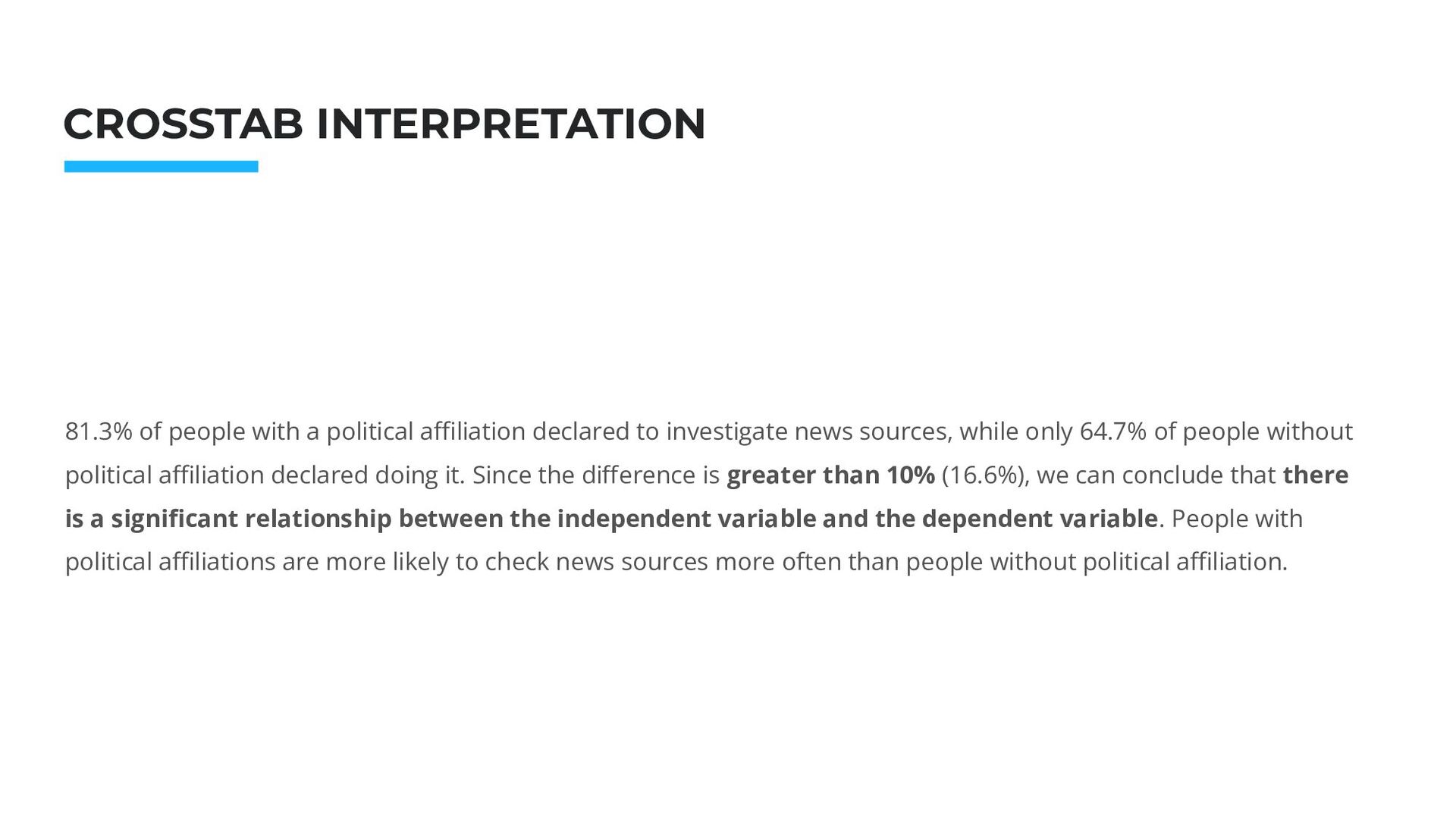
63. Photo: Startup Weekend Hackathon. Nov.2014 CROSSTAB INTERPRETATION 81.3% of people with a political affiliation declared to investigate news sources, while only 64.7% of people without political affiliation declared doing it. Since the difference is greater than 10% (16.6%), we can conclude that there is a significant relationship between the independent variable and the dependent variable. People with political affiliations are more likely to check news sources more often than people without political affiliation.
64. 4. MULTIVARIATE ANALYSIS
65. Photo: Startup Weekend Hackathon. Nov.2014 BIVARIATE ANALYSIS
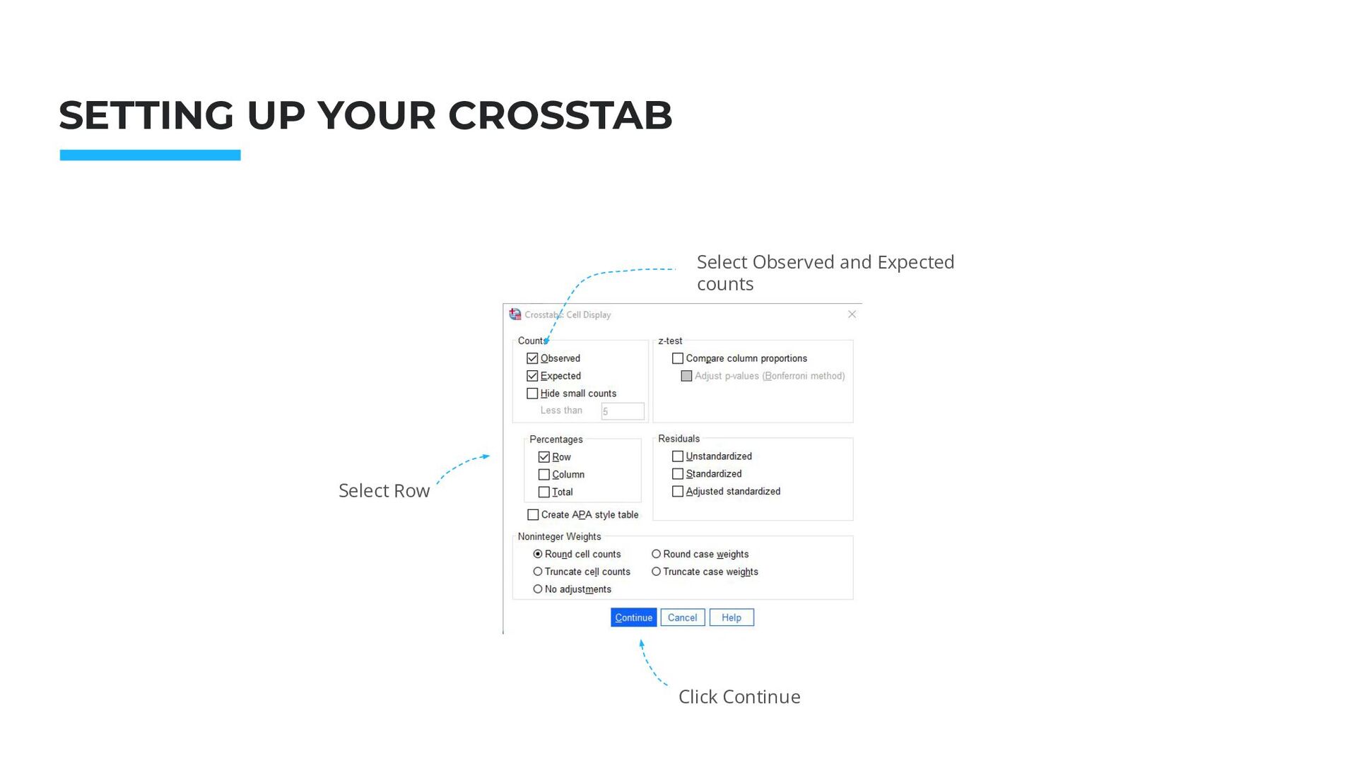
66. Photo: Startup Weekend Hackathon. Nov.2014 ADDING A CONTROL VARIABLE 1. Independent variable (recoded and cleaned) in the Rows 2. Dependent variable (recoded and cleaned) in the Columns 3. Control variable (recoded and cleaned) in the Layer box 4. Click Cells
67. Select Observed and Expected counts Photo: Startup Weekend Hackathon. Nov.2014 SETTING UP YOUR CROSSTAB Select Row Click Continue
68. Photo: Startup Weekend Hackathon. Nov.2014 BIVARIATE ANALYSIS ON CLEANED VARIABLES Control Variable (2 values only)
69. Photo: Startup Weekend Hackathon. Nov.2014 BIVARIATE ANALYSIS ON CLEANED VARIABLES Independent Variable (2 values only)
70. Photo: Startup Weekend Hackathon. Nov.2014 BIVARIATE ANALYSIS ON CLEANED VARIABLES Dependent Variable (2 values only)
71. Photo: Startup Weekend Hackathon. Nov.2014 IF YOU HAVE MORE THAN 2 VALUES IN ANY OF THE 3 VARIABLES, GO BACK TO DATA CLEANING AND MAKE SURE TO REMOVE ALL UNWANTED VALUES
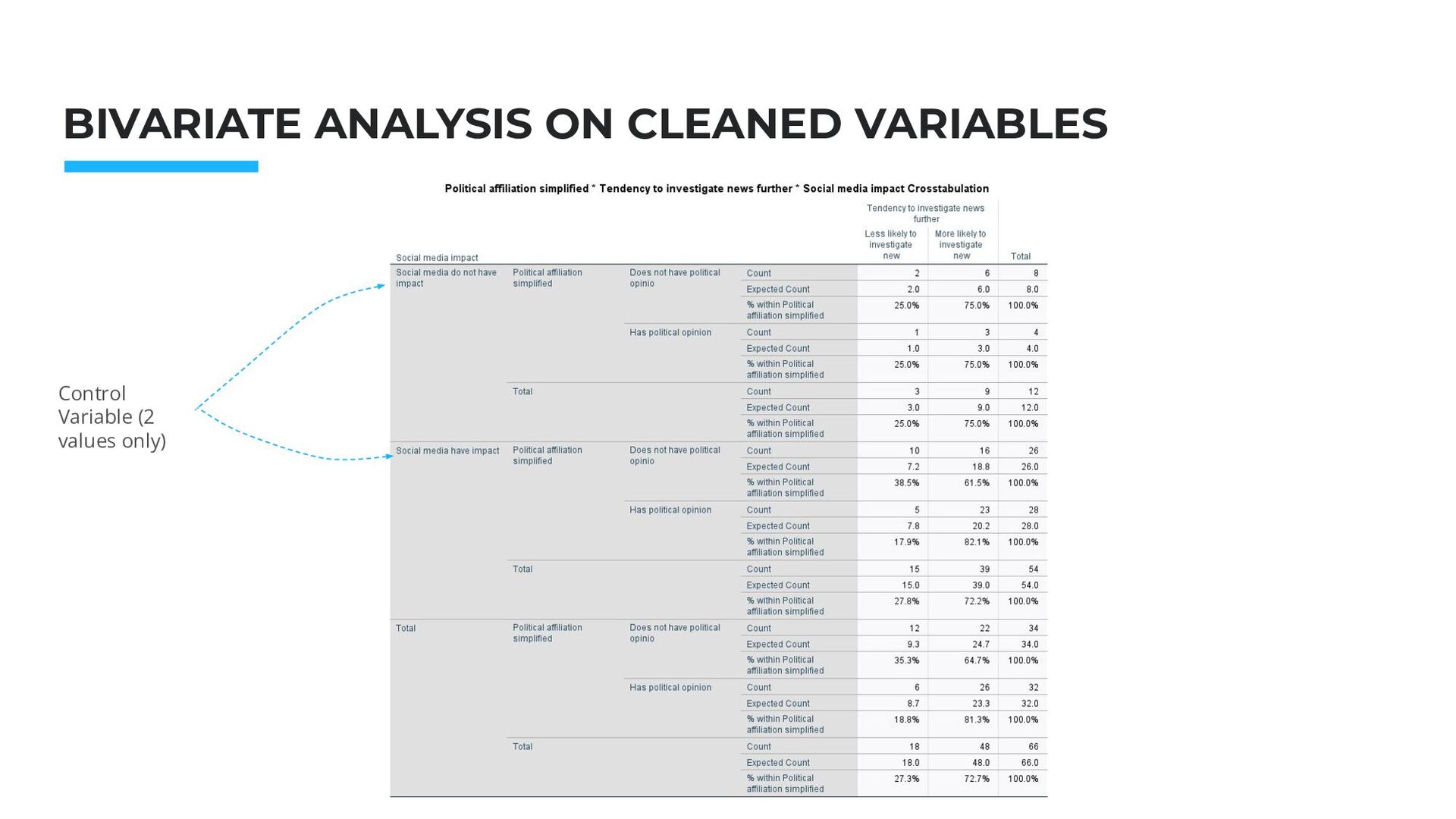
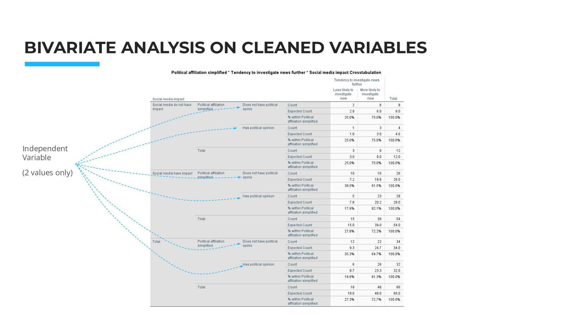
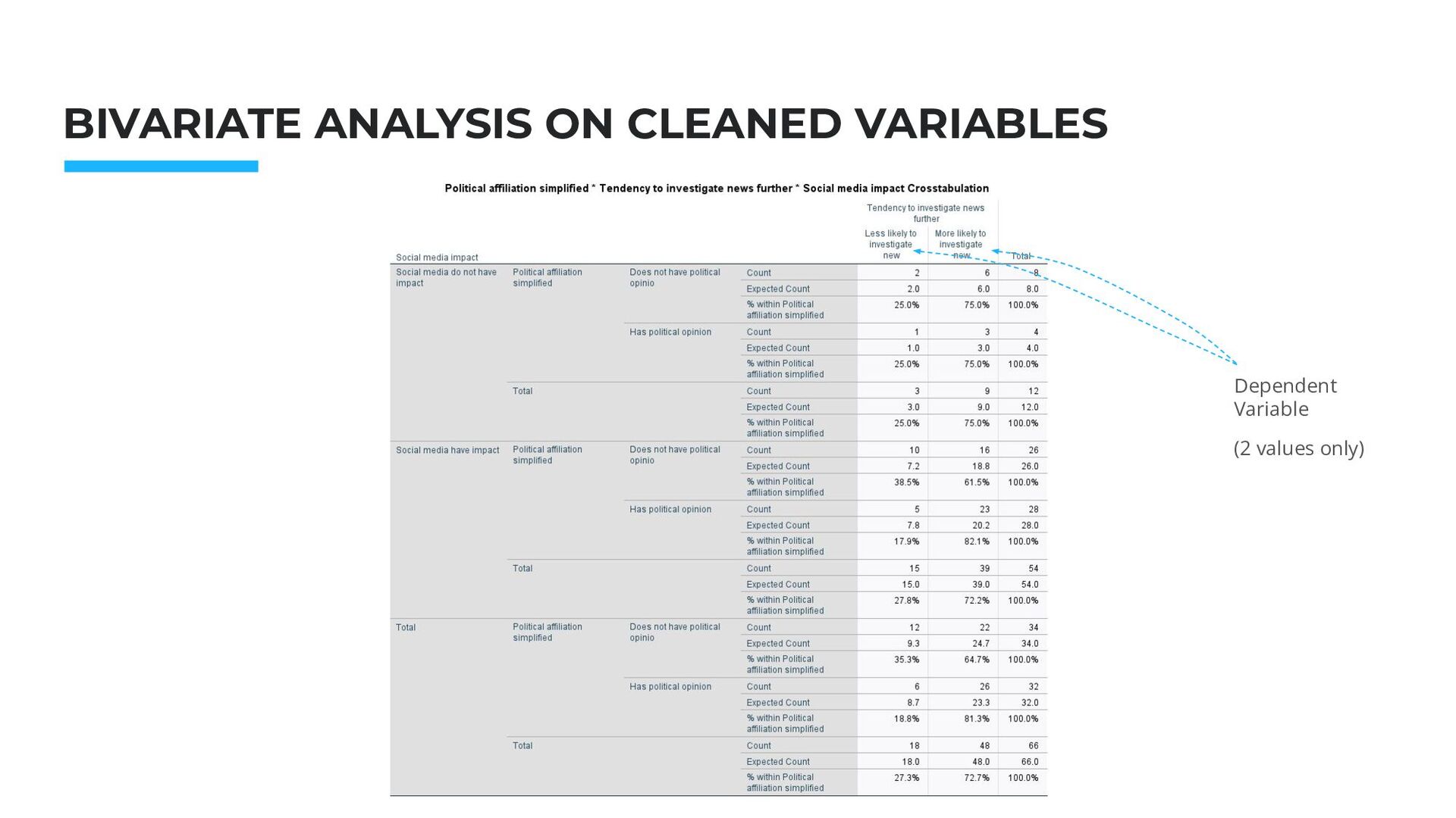
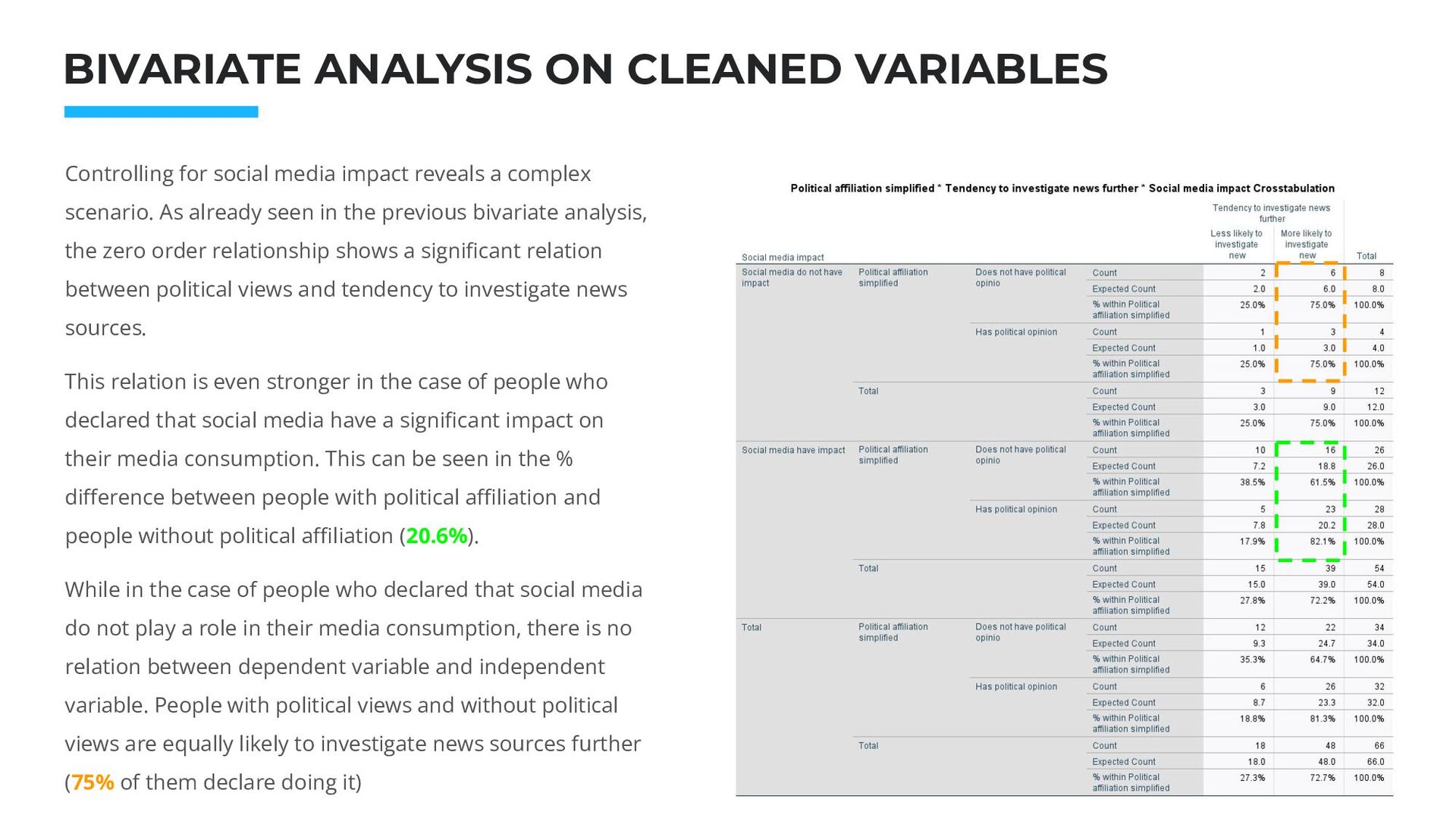
72. Photo: Startup Weekend Hackathon. Nov.2014 BIVARIATE ANALYSIS ON CLEANED VARIABLES Controlling for social media impact reveals a complex scenario. As already seen in the previous bivariate analysis, the zero order relationship shows a significant relation between political views and tendency to investigate news sources. This relation is even stronger in the case of people who declared that social media have a significant impact on their media consumption. This can be seen in the % difference between people with political affiliation and people without political affiliation (20.6%). While in the case of people who declared that social media do not play a role in their media consumption, there is no relation between dependent variable and independent variable. People with political views and without political views are equally likely to investigate news sources further (75% of them declare doing it)
73. Photo: Startup Weekend Hackathon. Nov.2014 INTERPRETING THE RESULTS See Week 7 slides for instructions on how to read a multivariate analysis crosstable. If you want to go the extra mile, and if possible, try to describe the relation between variables using the models described in Prof.Al-Rawi Week 8 lecture (specification, interpretation, explanation, replication, suppressor variable, distorter variable).
74. Photo: Startup Weekend Hackathon. Nov.2014 Congratulations, you have successfully completed the SPSS part of Assignment 3
75. Photo: Startup Weekend Hackathon. Nov.2014 Q&A
76. THANK YOU Alberto Lusoli alusoli@sfu.ca Office hour: Thursday, 12.30pm - 1.20pm (please book an appointment in advance via email).