The Geography of Educational Success and Progression

Kings College London - 5th June 2013

Transcript

1. Dr Alex D Singleton Department of Geography and Planning The Geography of Educational Success and Progression
2. Participation in “HE” has increased 0 175,000 350,000 525,000 700,000 1962 1964 1966 1968 1970 1972 1974 1976 1978 1980 1982 1984 1986 1988 1990 1992 1994 1996 1998 2000 2002 2004 2006 2008 Applicants Accepts Universities & Polytechnic Colleges Merged (UCCA & PCAS) ADAR / UCAS SWAS / UCAS
3. 0% 25% 50% 75% 100% 2002 2003 2004 2005 2006 2007 2008 Higher managerial and professio Lower managerial and professio Intermediate occupations Small employers and own accou Lower supervisory and technica Semi-routine occupations Routine occupations NS-SEC
4. 0% 25% 50% 75% 100% 2002 2003 2004 2005 2006 2007 2008 Higher managerial and professio Lower managerial and profession Intermediate occupations Small employers and own accou Lower supervisory and technical Semi-routine occupations Routine occupations Unknown NS-SEC
5. Overview • Prerequisites (Geographic referencing and context) – Building blocks – Indicators and geodemographics • Geodemographics and university participation • Can I recruit from anywhere? • Social sorting – school catchments • Turning data into information
6. GEOGRAPHIC REFERENCING AND CONTEXT Putting people on the map... % Level 4-5 Qualifications (2001 Census)
7. Households Building Blocks Students Postcodes ~15-25 addresses in a postcode Higher Geography
9. OA - Min: 40 households &100 people
10. LSOA - Min: 1,000 residents; 400 households. Av 1,500 residents
11. MSOA - Min size of 5,000 residents, 2,000 households
13. Indicators and Geodemographics • Linked to education data – Composite Measures: • IMD (LSOA) – Geodemographics – Output Area Classification (Output Area) – ACORN (Postcode) – POLAR – Rates of participation
16. http://www.hefce.ac.uk/whatwedo/wp/ourresearch/polar/ POLAR3 is based on the HE participation rates of those who entered HE during the 2005-06 to 2010-11 academic years
17. Waldo Tobler in front of the Newberry Library. Chicago, November 2007 (http://en.wikipedia.org/wiki/ Waldo_R._Tobler) First Law of Geography "Everything is related to everything else, but near things are more related to each other” http://en.wikipedia.org/wiki/University_of_California,_Santa_Barbara
18. http://www.nytimes.com/2010/05/24/arts/24iht-design24.html
19. Description BLACK: Lowest class. Vicious, semi-criminal. DARK BLUE: Very poor, casual. Chronic want. LIGHT BLUE: Poor. 18s. to 21s. a week for a moderate family PURPLE: Mixed. Some comfortable others poor PINK: Fairly comfortable. Good ordinary earnings. RED: Middle class. Well-to-do. YELLOW: Upper-middle and Upper classes. Wealthy.
20. •Technique developed in 1970’s attributed to Richard Webber •Identify similar neighborhoods •Target urban deprivation Funding •Public Sector – Government •Enumeration District Level •Moved to CACI •Linked ED to Postcode •ACORN (Private Sector) •Moved to Experian •MOSAIC (Private sector) Origins of Geodemographics
21. Output Area Classification: Liverpool
22. Moderate Means ! This category contains much of what used to be the country’s industrial heartlands. Many people are still employed in traditional, blue-collar occupations. Others have become employed in service and retail jobs as the employment landscape has changed. ! In the better off areas, incomes are in line with the national average and people have reasonable standards of living. However, in other areas, where levels of qualifications are low, incomes can fall below the national average. There are also some isolated pockets of unemployment and long-term illness. ! This category also includes some neighbourhoods with very high concentrations of Asian families on low incomes. ! Most housing is terraced, with two or three bedrooms, and largely owner occupied. It includes many former council houses, bought by their tenants in the 1980s. Overall, the people in this category have modest lifestyles, but are able to get by.
24. Students Achieving 5 A*-C Grade 75% 35%
25. GEODEMOGRAPHICS AND HE PARTICIPATION Social and spatial characteristics Output Area Classification
28. Data Integration DCSF Key Stage 5 HESA (0) HESA (+1) HESA (+2) 2004 ~50% ~20% ~5% Direct Entry Gap Year Gap Years National Targets = 18-30 Age Range
29. Student Flows into HE 2004 2005 2006 Overall % of KS5 51.3 20.9 4.5 72.3 % of KS4 20.2 10.4 3.5 32.0 2002 2004
30. HE Progression Rate with 95% Confidence Intervals (%) 0 18 35 53 70 1 2 3 4 5 6 7 8 9 10 11 12 13 14 15 16 17 18 19 20 21 22 23 24 25 26 27 28 29 30 31 32 33 34 35 36 37 38 39 40 41 42 43 44 45 46 47 48 49 50 51 52 53 54 55 56 Wealthy Achievers Urban Prosperity Comfortably Off Moderate Means Hard Pressed Inner City Adversity Asian Communities Home owning Asian family areas Low income, singles, small rented flats Low income, singles, small rented flats
31. 0.0 1.0 2.0 3.0 4.0 5.0 6.0 1A:Wealthy Executives 1B:Affluent Greys 1C:Flourishing Families 2A:Prosperous Professionals 2B:Educated Urbanites 2C:Aspiring Singles 3A:Starting Out 3B:Secure Families 3C:Settled Suburbia 3D:Prudent Pensioners 4A:Asian Communities 4B:Post-Industrial Families 4C:Blue-Collar Roots 5A:Struggling Families 5B:Burdened Singles 5C:High-Rise Hardship 5D:Inner City Adversity Medicine and Dentistry Subject Profiles Medicine and Dentistry
32. 0.0 2.0 4.0 6.0 8.0 10.0 12.0 14.0 1A:Wealthy Executives 1B:Affluent Greys 1C:Flourishing Families 2A:Prosperous Professionals 2B:Educated Urbanites 2C:Aspiring Singles 3A:Starting Out 3B:Secure Families 3C:Settled Suburbia 3D:Prudent Pensioners 4A:Asian Communities 4B:Post-Industrial Families 4C:Blue-Collar Roots 5A:Struggling Families 5B:Burdened Singles 5C:High-Rise Hardship 5D:Inner City Adversity Mathematical and Computer Sciences Subject Profiles Mathematical and Computer Sciences
33. A1-Medicine K4-Planning
34. Subjects & Participation in HE • Staggering differences in student characteristics between different courses of study over numerous measures – Social Class – Geodemographics – Polar – Etc... • Prior attainment strongly influences these patterns
35. CAN I RECRUIT FROM ANYWHERE? Output Area Classification
37. Can I recruit from anywhere? All 04 Acceptances Average Distance Miles 0.00 30.00 60.00 90.00 120.00 Geodemographic Sub-Type 1a1 1a2 1a3 1b1 1b2 1c1 1c2 1c3 2a1 2a2 2b1 2b2 3a1 3a2 3b1 3b2 3c1 3c2 4a1 4a2 4b1 4b2 4b3 4b4 4c1 4c2 4c3 4d1 4d2 5a1 5a2 5b1 5b2 5b3 5b4 5c1 5c2 5c3 6a1 6a2 6b1 6b2 6b3 6c1 6c2 6d1 6d2 7a1 7a2 7a3 7b1 7b2 Blue Collar Communities City Living Countryside Prospering Suburbs Constrained by Circumstances Typical Traits Multicultural Average Distance from applicant home to accepting institution
38. Distance 4 (Prospering Suburbs) No of People per bin 0.0000 2500.0000 5000.0000 7500.0000 10000.0000 Distance /km (20km bins) 0 150 300 450 600 7 (Multicultural) No of People per bin 0.0000 3000.0000 6000.0000 9000.0000 12000.0000 Distance /km (20km bins) 0 150 300 450 600
39. Distance 3 (Countryside) No of People per bin 0.0000 1500.0000 3000.0000 4500.0000 6000.0000 Distance /km (20km bins) 0 150 300 450 600 2 (City Living) 0.0000 500.0000 1000.0000 1500.0000 2000.0000 Distance /km (20km bins) 0 150 300 450 600
40. Spatial Interaction Modelling • A classic gravity model – Analogous to Newton’s 
 Law of Universal 
 Gravitation • Distance (or cost) decay 
 is always a key component – Tobler’s “first law of geography”
41. Spatial Interaction Modelling & HE • Sij = Ai km ei km Pi k (Wj mh)αkm exp(-βkm cij k) • This is the singly-constrained form – Finite number of school students go to university – No restriction on places at university – Doubly-constrained version is quite similar to look at • W is the “attractiveness” of the institution Sij = flow from school located at i to university located at j A, alpha and beta = constants k = geodemographic m = subject h = university c = cost of going from location i to j, for the k demographic (equivalent to d, the distance) e = subject demand P = population of the school W = attractiveness
42. Origin Side • National Pupil Database (NPD) – Home OAs (state only) – Used school OA for private schools – Includes attainment • Individual Learning Records (ILR) – For sixth-form colleges – Home postcodes – Includes attainment • OAC
43. Destination Side • HESA Individual Student Records – Subjects – Home postcodes – A-Level point score – Nearly everything needed for modelling the flows, but excludes those who didn’t go to university
44. Results • Simple Java GUI to show the matrix of results – visually spot good/poor matches – refine model parameters – rerun
45. Results – Norfolk Schools to Universities
46. Results – Schools to University of Manchester
47. Distance • Distance has a huge impact on where you will likely go to university • Interacts very strongly with the type of area in which you live – And – where this area is located relative to university / course provision
48. SOCIAL SORTING – SCHOOL CATCHMENTS Where can I go to school? Catchment Map of E Leeds
54. School Catchment Areas
57. School Catchment Areas Cheltenham Kingsmead School Mosaic Profile KS4 Index (Base 100) 0 75 150 225 300 Symbols of Success Happy Families Suburban Comfort Ties of Community Urban Intelligence Welfare Borderline Municipal Dependenc Blue Collar Enterprise Twilight Subsistence Grey Perspectives Rural Isolation Pates Grammar School Mosaic Profile KS4 Index (Base 100) 0 100 200 300 400 Symbols of Success Happy Families Suburban Comfort Ties of Community Urban Intelligence Welfare Borderline Municipal Dependenc Blue Collar Enterprise Twilight Subsistence Grey Perspectives Rural Isolation A high performing school in Cheltenham A low performing school in Cheltenham
58. Social Sorting • Where you live has a strong bearing on which schools you can access in many areas – House prices • Regional differences
59. TURNING DATA INTO INFORMATION Profiling for the public Target Schools for University Oxford
61. Process • Lookup average distance geodemographic group travels to selected university – Select all schools within this range • Target group = those geodemographic groups less likely to participate – Colour schools red where these are over represented (index > 120) • Scale points by the volume of target pupils
71. What is needed… • Better linked data • Better tools to help allocate limited resources
72. Research Agenda • Refine HE Model – Fee Price – Course – University Closure / Merger – Course Offerings – Impact on WP
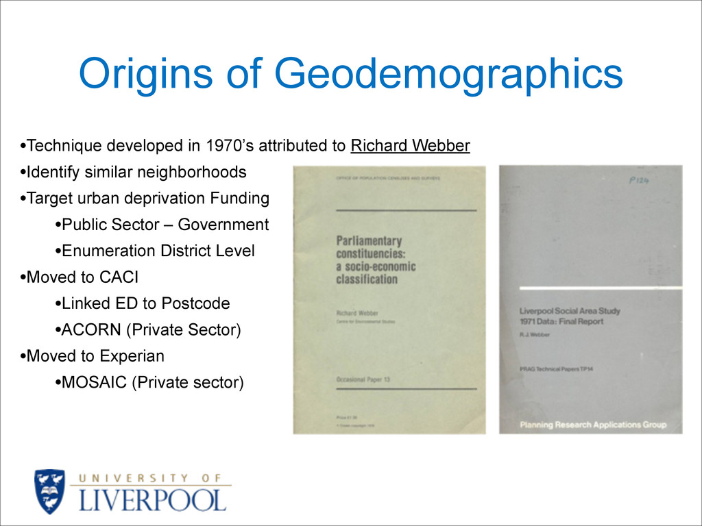
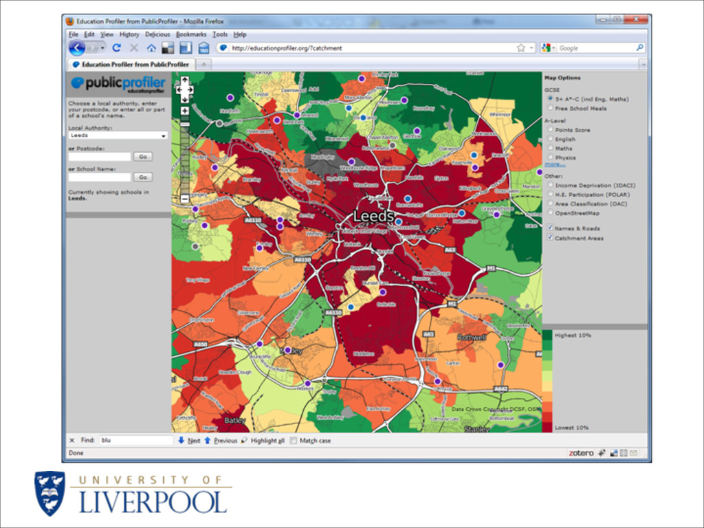
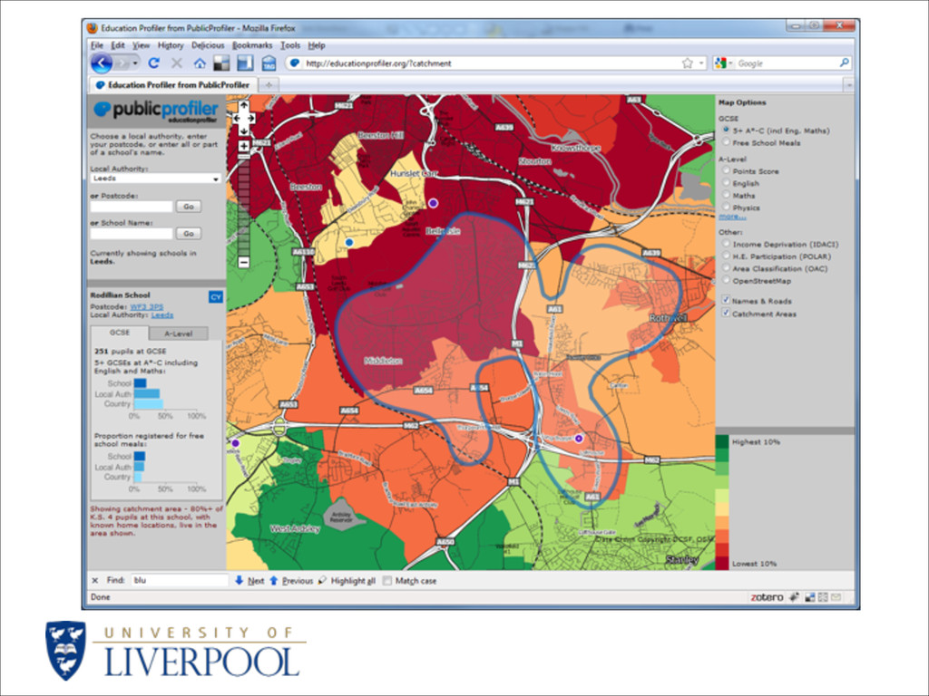
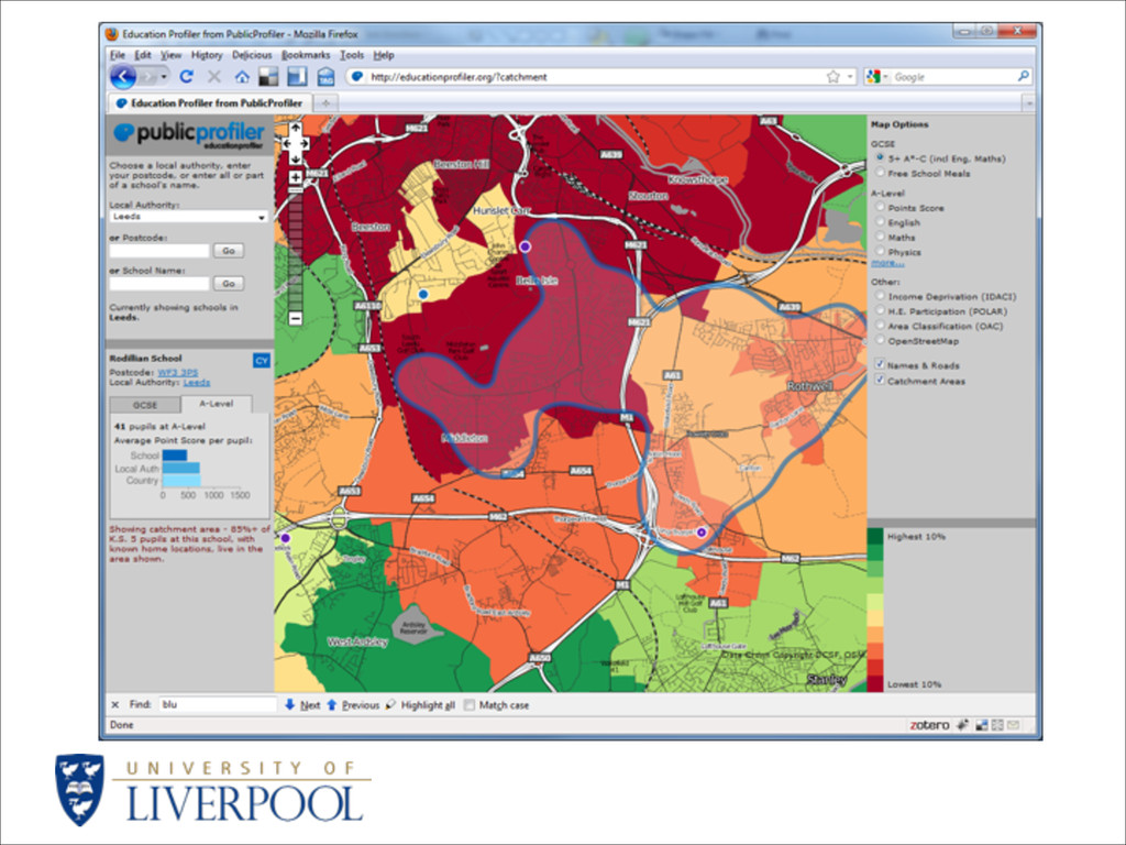
73. References 1. Singleton, A.D. 2012. “The Geodemographics of Access and Participation in Geography.” The Geographical Journal 178 (3): 216–229. http://dx.doi.org/10.1111/j.1475-4959.2012.00467.x. 2. Singleton, A.D., Alan G Wilson, and Oliver O’Brien. 2012. “Geodemographics and Spatial Interaction: An Integrated Model for Higher Education.” Journal of Geographical Systems 14 (2): 223–241. http://dx.doi.org/10.1007/ s10109-010-0141-5. 3. Brunsdon, Chris, Paul Longley, A.D. Singleton, and David Ashby. 2011. “Predicting Participation in Higher Education: a Comparative Evaluation of the Performance of Geodemographic Classifications.” Journal of the Royal Statistical Society: Series A (Statistics in Society) 174 (1): 17–30. http://dx.doi.org/10.1111/j.1467-985X. 2010.00641.x. 4. Singleton, A.D., P.A. Longley, Rebecca Allen, and Oliver O’Brien. 2011. “Estimating Secondary School Catchment Areas and the Spatial Equity of Access.” Computers, Environment and Urban Systems 35 (3): 241–249. http:// dx.doi.org/10.1016/j.compenvurbsys.2010.09.006. 5. Harris, Richard, A.D. Singleton, Daniel Grose, Chris Brunsdon, and P.A. Longley. 2010. “Grid-enabling Geographically Weighted Regression: A Case Study of Participation in Higher Education in England.” Transactions in GIS 14 (1): 43–61. http://dx.doi.org/10.1111/j.1467-9671.2009.01181.x 6. Singleton, A.D. 2010. “The Geodemographics of Educational Progression and Their Implications for Widening Participation in Higher Education.” Environment and Planning A 42 (11): 2560–2580. http://dx.doi.org/10.1068/ a42394. 7. Singleton, A., 2010. Educational Opportunity : the Geography of Access to Higher Education, Farham: Ashgate. 8. Singleton, A.D. 2009. “Data Mining Course Choice Sets and Behaviours for Target Marketing of Higher Education.” Journal of Targeting, Measurement and Analysis for Marketing 17 (3): 157–170. http://dx.doi.org/10.1057/jt. 2009.13. 9. Singleton, A.D., and P.A. Longley. 2009. “Creating Open Source Geodemographics - Refining a National Classification of Census Output Areas for Applications in Higher Education.” Papers in Regional Science 88 (3): 643–666. http://dx.doi.org/10.1111/j.1435-5957.2008.00197.x. ! ! ! !
74. www.alex-singleton.com