AAGW3 - Carlo Azzarri - The new sub-national poverty map

Transcript

1. University of Minnesota St. Paul, December 20, 2012
2. Background • IFPRI with CIAT were using constant ratios by administrative unit to infer poverty rates from national poverty lines to PPP lines
3. How we were doing Green maps = we had the data Gray maps = we wanted to estimate $1 per day Poverty line Headcount (%) National Poverty line Headcount (%) National poverty Line headcount % $1 per day Poverty line Headcount (%) RATIO Apply RATIO above by district
4. 10 15 17 11 19 Number of poor (HC_NAL….77 total number of poor in country, according to map and GPW3_2005) % of poor (no. of poor in district divided by total number of poor in country) .13 .14 .19 .22 .25 Number of poor at $1.25 poverty Line according to POVCALNET 99 * % of poor (no. of poor in district divided by total number of poor in country) .13 .14 .19 .22 .25 Estimated $1.25 poverty line = 77, no. of poor at national poverty line 13 19 14 22 25 ?
5. nat PL (19.1 MTS) $1.25PPP (18.1 MTS) $2PPP (29.0 MTS) 0 .2 .4 .6 .8 1 0 10 20 30 40 50 pc-consumption North Centre South
6. nat PL (19.1 MTS) $1.25PPP (18.1 MTS) $2PPP (29.0 MTS) 0 .2 .4 .6 .8 1 0 10 20 30 40 50 pc-consumption Niassa Maputo city Maputo province
7. ISO3_CODE Country name Survey used # sub-national units PHC $1.25 PHC $2 GINI BFA BURKINA FASO EICM, 2003 13 63.02 82.69 45.88 BDI BURUNDI CWIQ, 2006 17 79.67 92.83 33.27 CMR CAMEROON EICM, 2007 12 6.76 27.05 38.96 CIV COTE D’IVOIRE ENV, 2002-3 11 22.81 47.8 48.28 COD D.R.CONGO 1-2-3, 2004-5 11 57.06* 78.99* 42.15* ETH ETHIOPIA HICE, 2004-5 10 37.07 77.32 29.76 GMB GAMBIA PS, 1998 7 68.57 83.84 49.18 GHA GHANA GLSS, 2005 10 29.49 54.29 42.76 KEN KENYA IHBS, 2005 69 18.43 41.56 47.62 LSO LESOTHO HBS, 2002-3 10 46.10 64.76 52.44 MDG MADAGASCAR EPM, 2005 22 68.91 89.08 35.87 MWI MALAWI IHS, 2004-5 26 73.99 89.61 39.00 MLI MALI HIS, 2006 9 51.91 75.53 39.11 MRT MAURITANIA EPCV, 2000 13 22.69 47.03 39.02 MOZ MOZAMBIQUE IAF, 2002-3 11 75.86 89.03 47.74 NER NIGER ENBC, 2007 8 38.67 72.81 34.00 NGA NIGERIA NLSS, 2003-4 37 66.23 84.95 43.67 RWA RWANDA EICV, 2005-6 12 69.49 84.39 52.04 SEN SENEGAL ESAM, 2001 10 44.01 70.68 41.31 SSD SOUTH SUDAN NBHS, 2009 10 48.05 68.92 45.54 SWZ SWAZILAND HIES, 1995-6 6 79.85 88.78 61.99 TZA TANZANIA HBS, 2007 21 66.14 86.29 37.82 UGA UGANDA UNHS, 2005 4 51.06 75.41 40.83 ZMB ZAMBIA LMCS, 2006 9 69.61 82.43 57.70
10. …by AEZ …by farming system
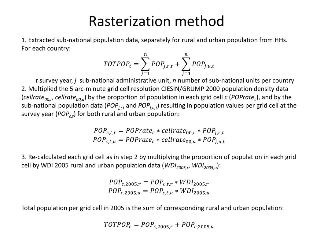
11. Rasterization method 1. Extracted sub-national population data, separately for rural and urban population from HHs. For each country: = ,, =1 + ,, =1 t survey year, j sub-national administrative unit, n number of sub-national units per country 2. Multiplied the 5 arc-minute grid cell resolution CIESIN/GRUMP 2000 population density data (cellrate00,r , cellrate00,u ) by the proportion of population in each grid cell c (POPratec ), and by the sub-national population data (POPj,r,t and POPj,u,t ) resulting in population values per grid cell at the survey year (POPc,t ) for both rural and urban population: ,, = ∗ 00, ∗ ,, ,, = ∗ 00, ∗ ,, 3. Re-calculated each grid cell as in step 2 by multiplying the proportion of population in each grid cell by WDI 2005 rural and urban population data (WDI2005,r , WDI2005,u ): ,2005, = ,, ∗ 2005, ,2005, = ,, ∗ 2005, Total population per grid cell in 2005 is the sum of corresponding rural and urban population: = ,2005, + ,2005,
12. Carlo, Elizabeth, Mel
13. Data harmonization • Countries: MWI (04/5), TZA (07/8), UGA (09/10), ETH (00/01), GHA (05/6) • Variables: demographic, socio-economic, livelihoods (income sources), spatial, area cultivated, production, yield, sales, irrigation, use of inputs, crop combination, livestock [by season, crop/animal type whenever possible] • Reports: MWI TZA UGA
14. Carlo, Elizabeth
15. Outline • Introduction and motivation • Conceptual framework • Objectives • Literature and methods • Data and pitfalls • Model(s) • Findings • Conclusions and roadmap • (Initial results on nutrition)
16. Introduction and motivation • Importance of livestock ->“the next food revolution” • Perceived low contribution of livestock to total income (and livelihoods) • Scarsity of quantitative and spatially- disaggregated livestock measures • Little use of integrated data and spatial micro- level models
17. Objectives • Providing policy-makers and analysts with reliable and detailed information on livestock • Improving the spatial resolution of information • Showing how integration of different data sources can greatly enhance analysis and knowledge • Using alternative method based on a wide array of data (surveys, census, satellite, FAO…)
18. Data • UNPS 09/10: 2,975 (2,375)* HHs from 322 EAs (out of 783 of the UNHS 05/06), nationally + Kampala&other urban, and rural Central, Eastern, Western, Northern representative. Two visits (one for cropping season), twelve-month period • UNLC 08: 964,047 HHs from all 80 districts (for a total of 8,870 EAs with at least 50 HHs/EA). Visit in February only • (ILRI, IFPRI/HarvestChoice, FAO spatial database) *45 interviews were not complete; 555 hhs are mover (364 are split-offs and 191 original movers)
19. Model/1 • Small Area Estimation (SAE): 1. identifying characteristics with common definitions (and distributions) in both NPS and NLC, used as potential explanatory variables (correlates) in a regression using the survey data: = ∗ + = +
20. Model/2 2. combining the results of the first-stage regression model with census variables: = ∗ + + • Assumptions: spatial correlation b/n EA and subcounty, area homogeneity • Predictors (X): farm size, pasture land, other land, # of livestock heads by type (including exotic/indigenous bulls, cows, calves, and small ruminants), # of eggs and liters of milk weekly produced, age and sex of household head, whether the household hired agricultural labor, dummies by agro-ecological zone, NDVI)
21. Findings: density of large ruminants/1 survey census
22. Findings: density of large ruminants/2 actual predicted R2 .56 Adj-R2 .56
23. Findings: per-capita liv. income PPP/1 R2 .24 Adj-R2 .20
24. Findings: per-capita liv. income PPP/2
25. Findings: share of livestock income/1 R2 .15 Adj-R2 .11
26. Findings: share of livestock income/2
27. Conclusions • Concrete possibility of combining multi-topic household surveys with specialized databases to estimate contribution of livestock to household livelihoods • Integration b/n different data sources allows for finer spatial resolution • Spatially-specific data have been successfully used for targeting poverty programs…potentially useful tool for informing livestock policy?
28. Roadmap • Through this method we can look at different outcomes, what are we after? • Using the “improved” livestock module in NPS 11-12 • Scaling-out to other countries: 1. Tanzania 2. Ethiopia 3. Malawi 4. Niger 5. Nigeria • Refining data: is there scope (and leverage, especially for census)?
29. Carlo, Elizabeth
30. T. F. Randolph et al., “Invited Review: Role of livestock in human nutrition and health for poverty reduction in developing countries,” Journal of Animal Science 85, (2007): 2791.
31. Non-owners: -meat/fish/dairy, -fruit, +meals outside 0 .2 .4 .6 .8 1 owner nonowner Share of Consumption from Multiple Food Sources Cereals Meat and Fish Eggs and Dairy Fruit Vegetables Nuts, Oils, and Fats Sugar and Beverages Other Restaurant
32. Non-poor: +meat/fish/dairy, +fruit, -vegetables 0 .2 .4 .6 .8 1 poor nonpoor Share of Consumption from Multiple Food Sources Cereals Meat and Fish Eggs and Dairy Fruit Vegetables Nuts, Oils, and Fats Sugar and Beverages Other Restaurant
33. Livestock share decreases with wealth