Lecture slides for Lecture 14 of the Saint Louis University Course Quantitative Analysis: Applied Inferential Statistics. These slides cover one-way ANOVA.
will be strict about this extended deadline so I can do a quick turnaround on feedback and generate your Lecture-16 grade summary. Lab 11 is due next Monday - there will be no problem set. Please focus on the final project! 1. FRONT MATTER ANNOUNCEMENTS A progress report was due today - please open an issue in your final project repo and let me know how things are progressing! Lab 11 is due next Monday - there will be no problem set. Please focus on the final project! Our finals week presentations will begin at 4pm - focus on keeping your presentation at 5-6 minutes so we can be done by 6pm!
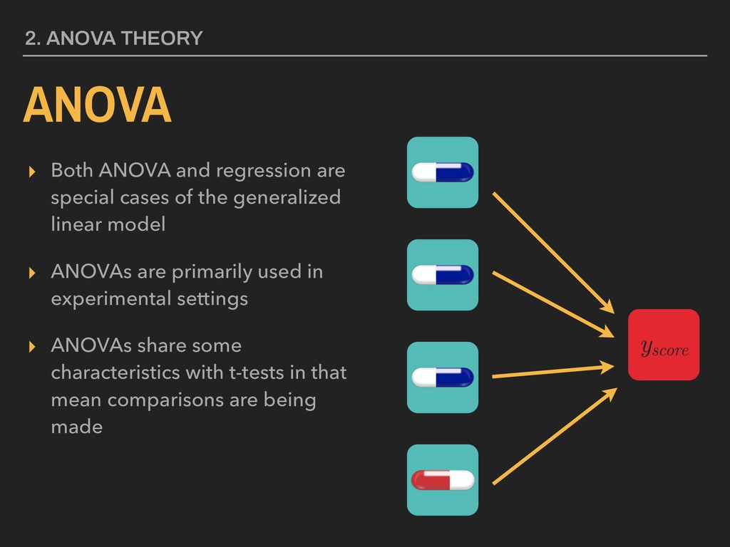
generalized linear model ▸ ANOVAs are primarily used in experimental settings ▸ ANOVAs share some characteristics with t-tests in that mean comparisons are being made 2. ANOVA THEORY ANOVA xc xa y xd xe
generalized linear model ▸ ANOVAs are primarily used in experimental settings ▸ ANOVAs share some characteristics with t-tests in that mean comparisons are being made 2. ANOVA THEORY ANOVA yscore
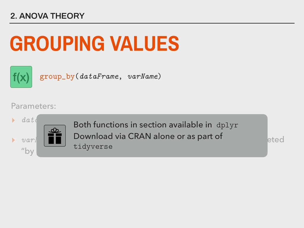
modified ▸ varName is the grouping variable that you want operations completed “by group” Both functions in section available in dplyr Download via CRAN alone or as part of tidyverse 2. ANOVA THEORY GROUPING VALUES Parameters: group_by(dataFrame, varName)
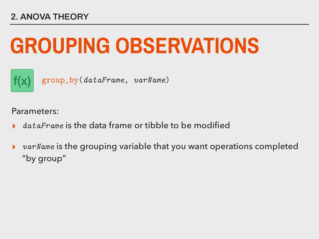
modified ▸ varName is the grouping variable that you want operations completed “by group” 2. ANOVA THEORY GROUPING OBSERVATIONS Parameters: group_by(dataFrame, varName)
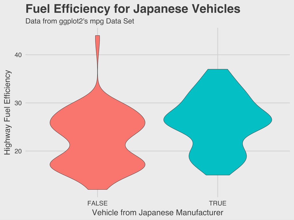
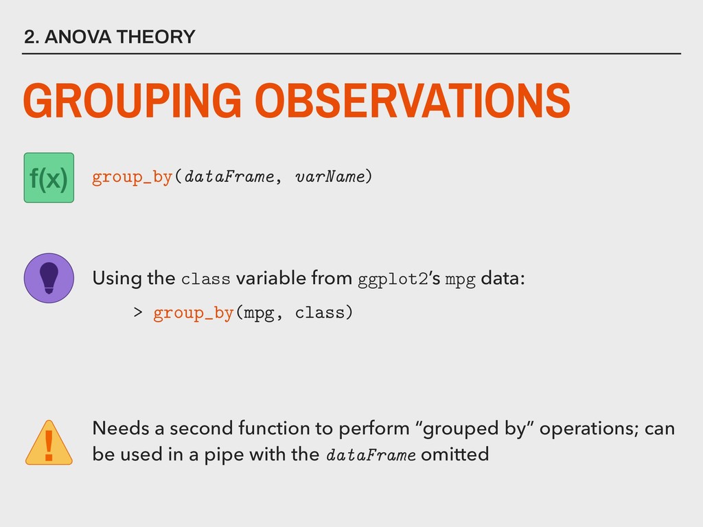
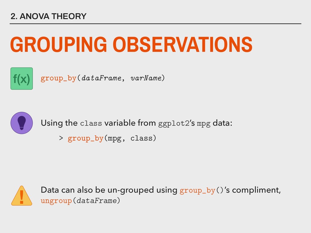
variable from ggplot2’s mpg data: > group_by(mpg, class) Needs a second function to perform “grouped by” operations; can be used in a pipe with the dataFrame omitted
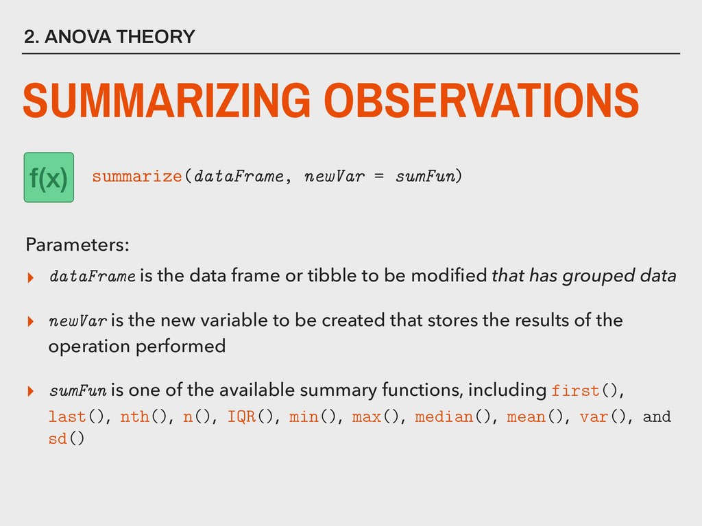
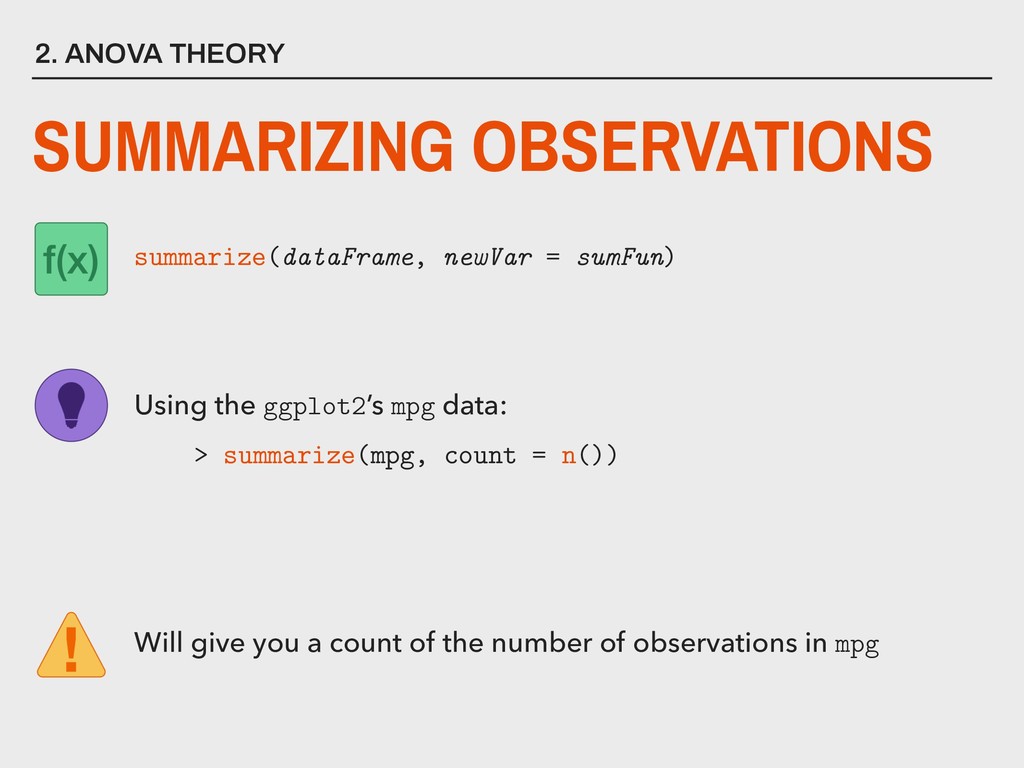
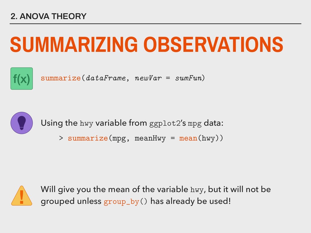
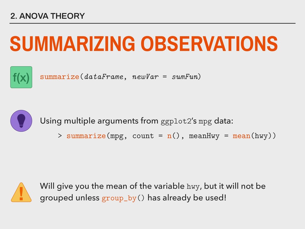
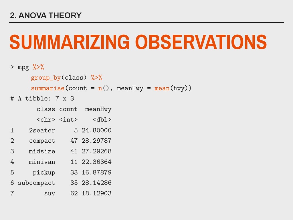
modified that has grouped data ▸ newVar is the new variable to be created that stores the results of the operation performed ▸ sumFun is one of the available summary functions, including first(), last(), nth(), n(), IQR(), min(), max(), median(), mean(), var(), and sd() 2. ANOVA THEORY SUMMARIZING OBSERVATIONS Parameters: summarize(dataFrame, newVar = sumFun)
the hwy variable from ggplot2’s mpg data: > summarize(mpg, meanHwy = mean(hwy)) Will give you the mean of the variable hwy, but it will not be grouped unless group_by() has already be used!
multiple arguments from ggplot2’s mpg data: > summarize(mpg, count = n(), meanHwy = mean(hwy)) Will give you the mean of the variable hwy, but it will not be grouped unless group_by() has already be used!
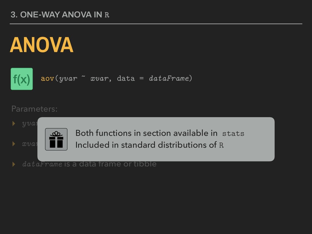
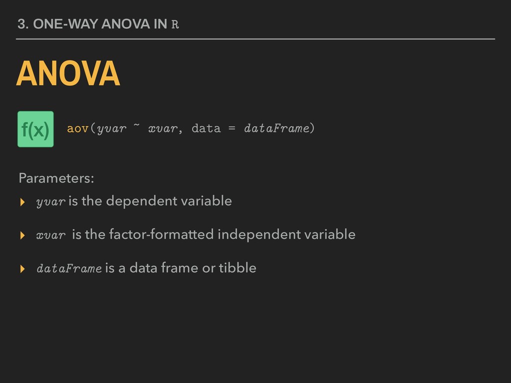
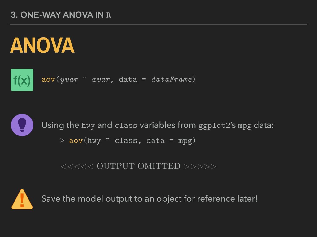
factor-formatted independent variable ▸ dataFrame is a data frame or tibble 3. ONE-WAY ANOVA IN R ANOVA Parameters: aov(yvar ~ xvar, data = dataFrame) Both functions in section available in stats Included in standard distributions of R
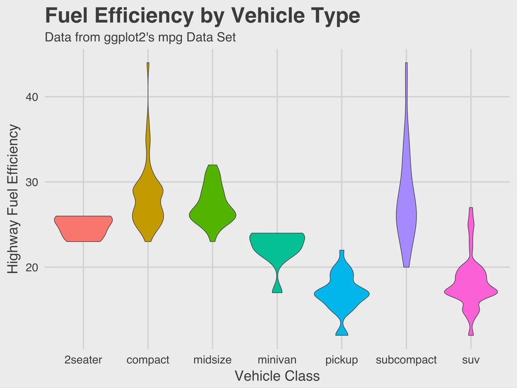
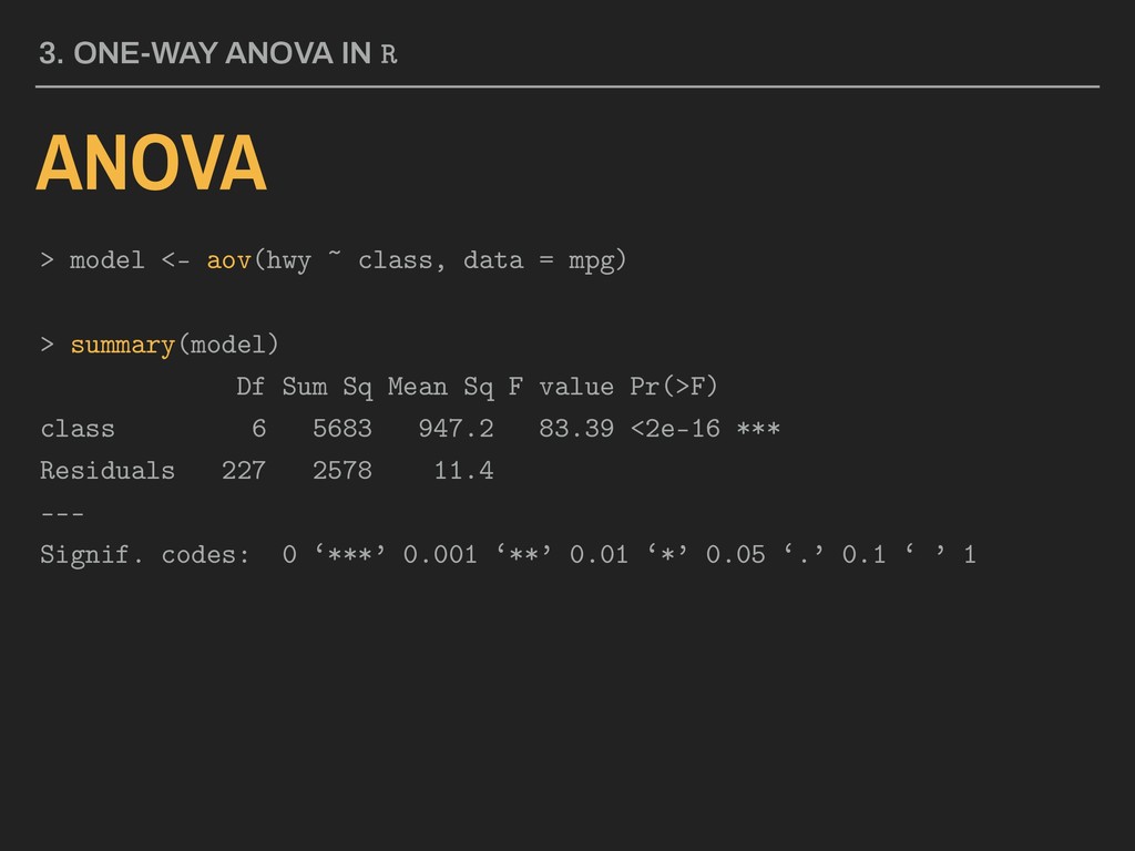
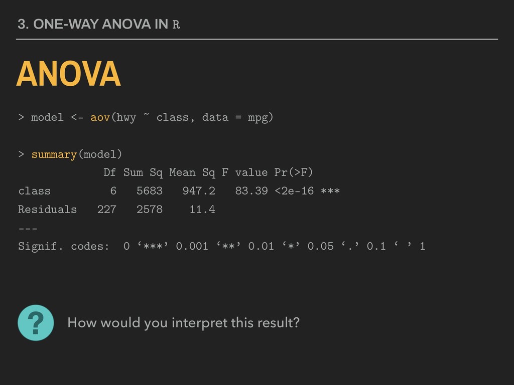
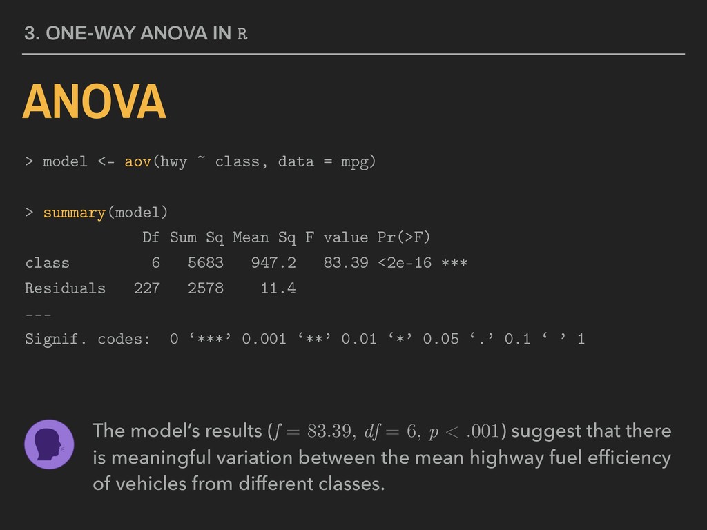
= dataFrame) Using the hwy and class variables from ggplot2’s mpg data: > aov(hwy ~ class, data = mpg) <<<<< OUTPUT OMITTED >>>>> Save the model output to an object for reference later!
> summary(model) Df Sum Sq Mean Sq F value Pr(>F) class 6 5683 947.2 83.39 <2e-16 *** Residuals 227 2578 11.4 --- Signif. codes: 0 ‘***’ 0.001 ‘**’ 0.01 ‘*’ 0.05 ‘.’ 0.1 ‘ ’ 1 3. ONE-WAY ANOVA IN R How would you interpret this result?
> summary(model) Df Sum Sq Mean Sq F value Pr(>F) class 6 5683 947.2 83.39 <2e-16 *** Residuals 227 2578 11.4 --- Signif. codes: 0 ‘***’ 0.001 ‘**’ 0.01 ‘*’ 0.05 ‘.’ 0.1 ‘ ’ 1 3. ONE-WAY ANOVA IN R The model’s results (f = 83.39, df = 6, p < .001) suggest that there is meaningful variation between the mean highway fuel efficiency of vehicles from different classes.
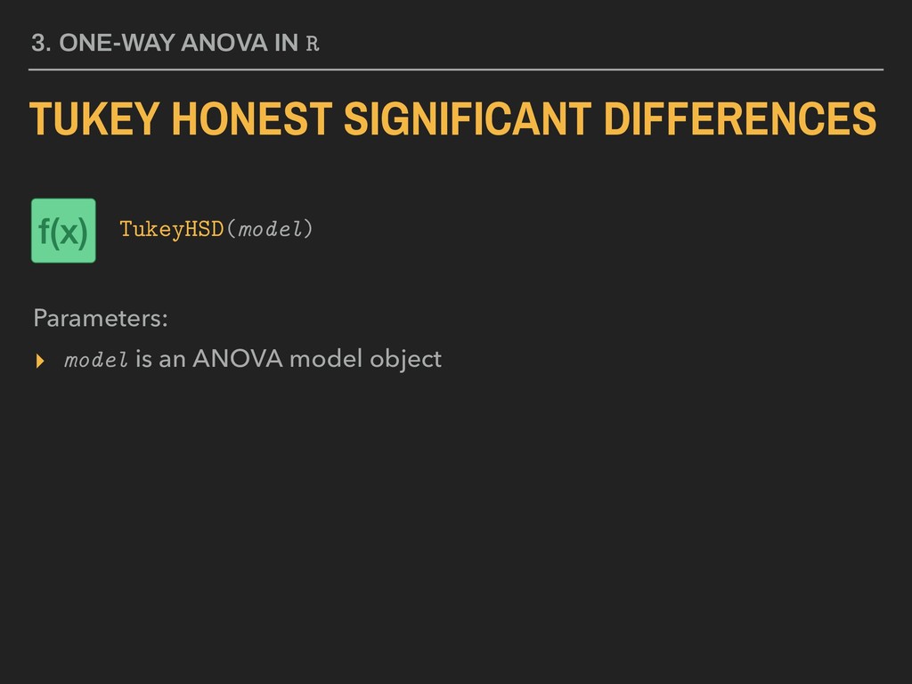
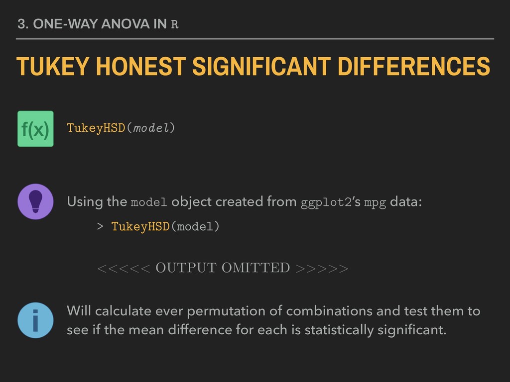
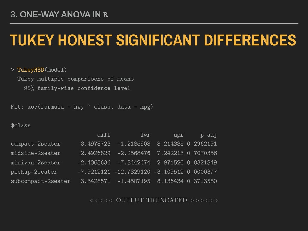
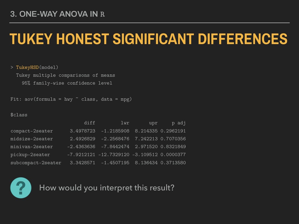
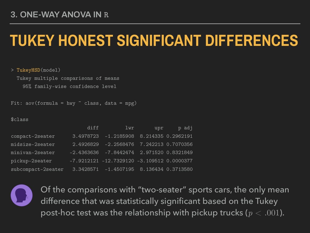
Using the model object created from ggplot2’s mpg data: > TukeyHSD(model) <<<<< OUTPUT OMITTED >>>>> Will calculate ever permutation of combinations and test them to see if the mean difference for each is statistically significant.
the comparisons with “two-seater” sports cars, the only mean difference that was statistically significant based on the Tukey post-hoc test was the relationship with pickup trucks (p < .001). > TukeyHSD(model) Tukey multiple comparisons of means 95% family-wise confidence level Fit: aov(formula = hwy ~ class, data = mpg) $class diff lwr upr p adj compact-2seater 3.4978723 -1.2185908 8.214335 0.2962191 midsize-2seater 2.4926829 -2.2568476 7.242213 0.7070356 minivan-2seater -2.4363636 -7.8442474 2.971520 0.8321849 pickup-2seater -7.9212121 -12.7329120 -3.109512 0.0000377 subcompact-2seater 3.3428571 -1.4507195 8.136434 0.3713580
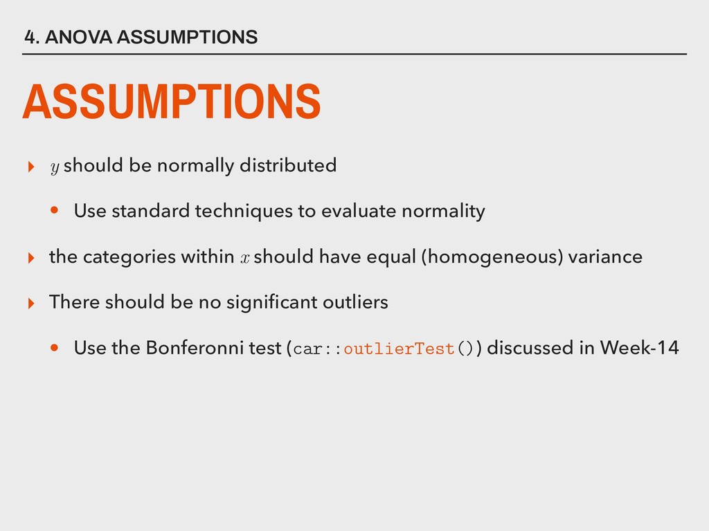
• Use standard techniques to evaluate normality ▸ the categories within x should have equal (homogeneous) variance ▸ There should be no significant outliers • Use the Bonferonni test (car::outlierTest()) discussed in Week-14
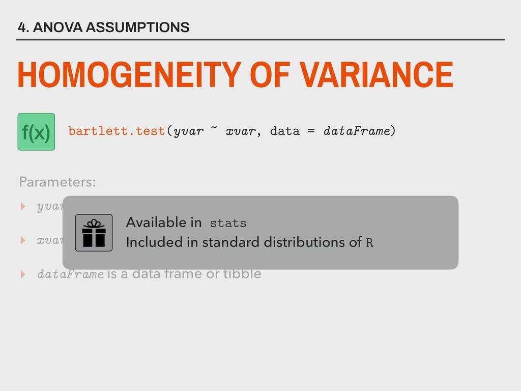
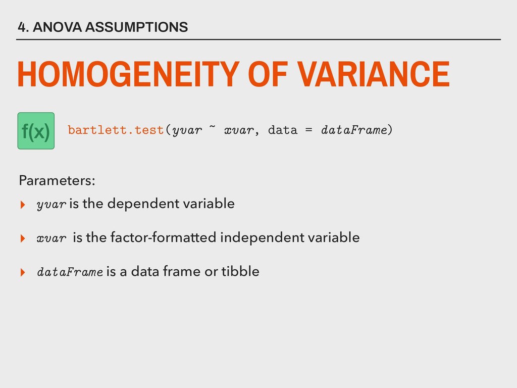
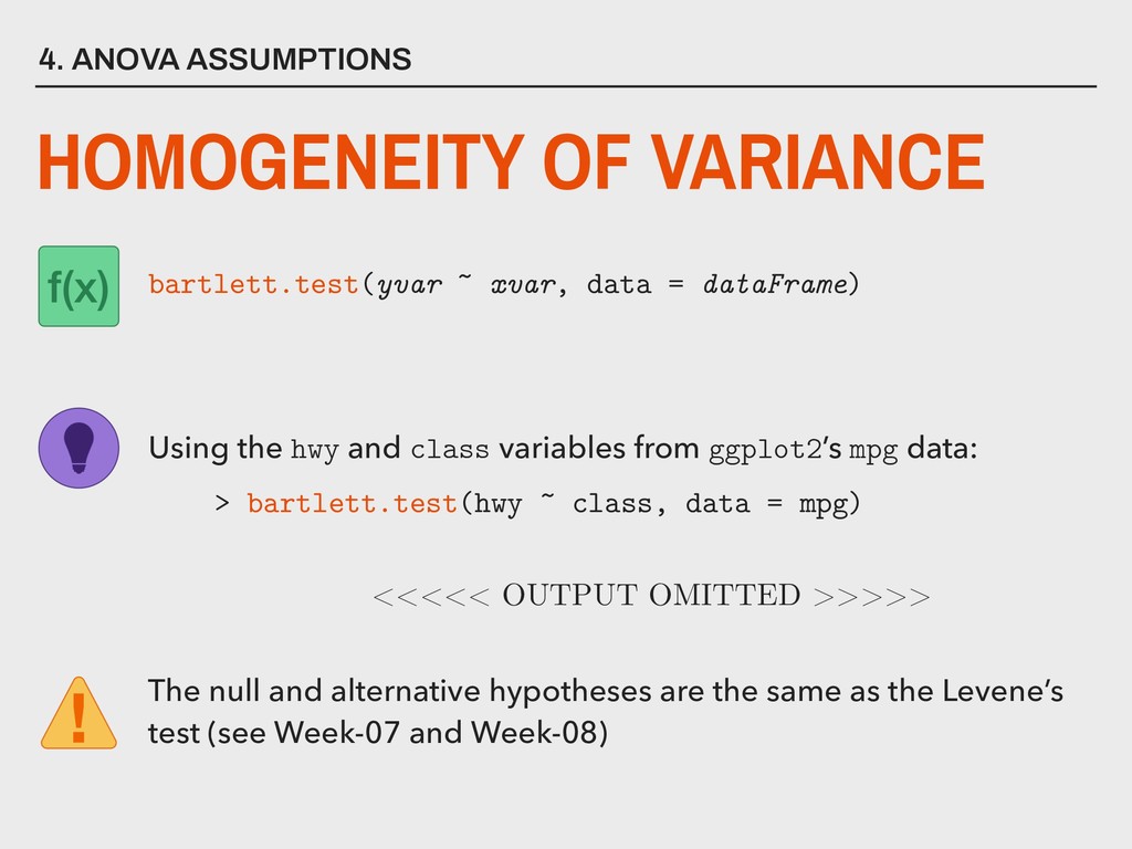
factor-formatted independent variable ▸ dataFrame is a data frame or tibble Available in stats Included in standard distributions of R 4. ANOVA ASSUMPTIONS HOMOGENEITY OF VARIANCE Parameters: bartlett.test(yvar ~ xvar, data = dataFrame)
factor-formatted independent variable ▸ dataFrame is a data frame or tibble 4. ANOVA ASSUMPTIONS HOMOGENEITY OF VARIANCE Parameters: bartlett.test(yvar ~ xvar, data = dataFrame)
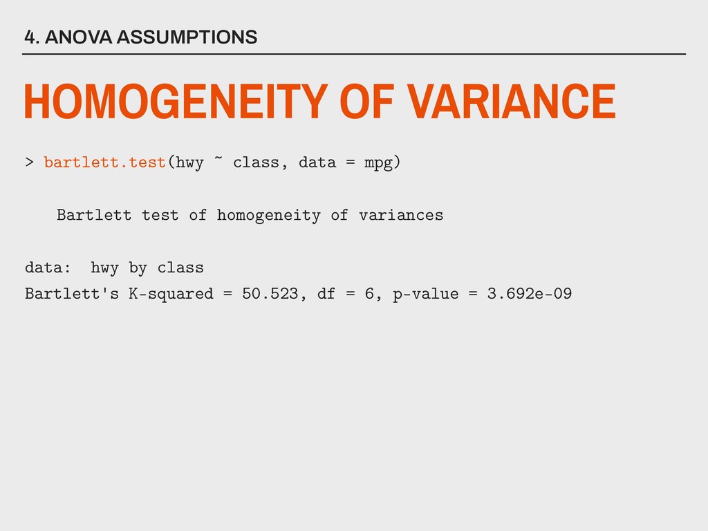
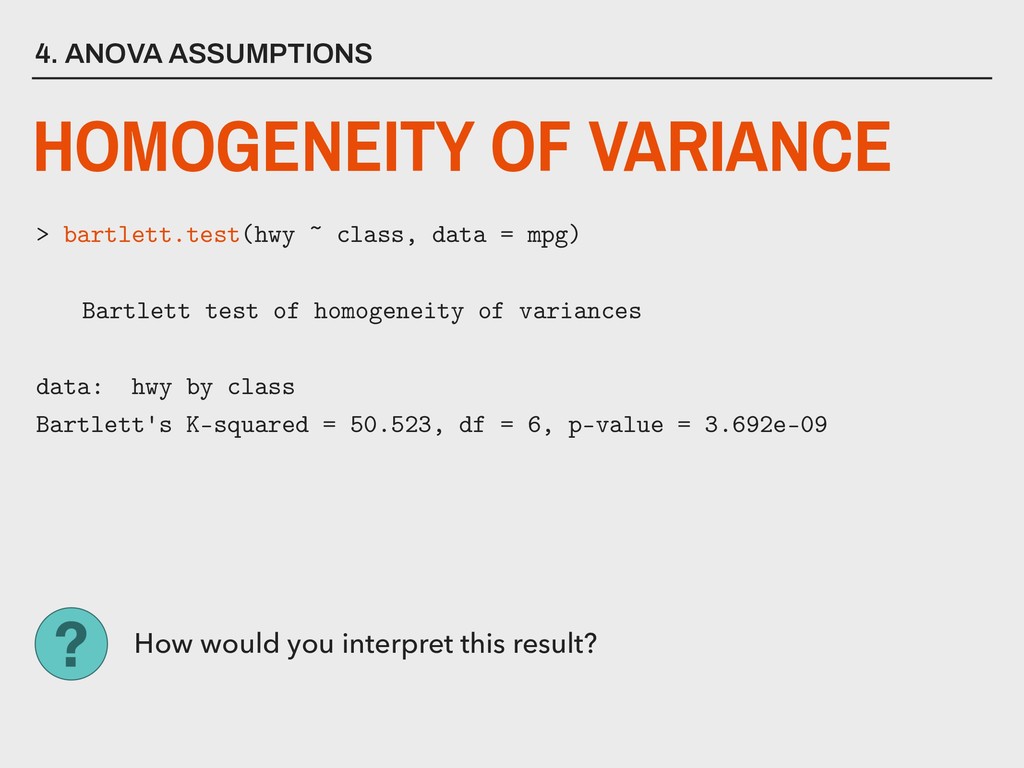
= dataFrame) Using the hwy and class variables from ggplot2’s mpg data: > bartlett.test(hwy ~ class, data = mpg) <<<<< OUTPUT OMITTED >>>>> The null and alternative hypotheses are the same as the Levene’s test (see Week-07 and Week-08)
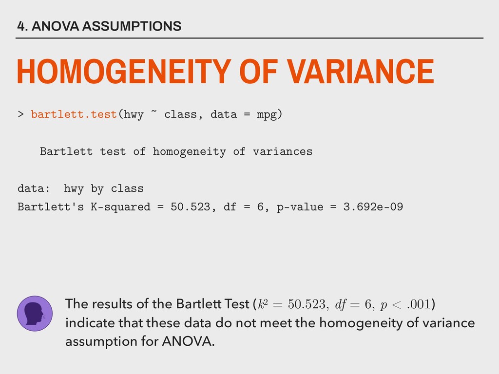
OF VARIANCE > bartlett.test(hwy ~ class, data = mpg) Bartlett test of homogeneity of variances data: hwy by class Bartlett's K-squared = 50.523, df = 6, p-value = 3.692e-09
data = mpg) Bartlett test of homogeneity of variances data: hwy by class Bartlett's K-squared = 50.523, df = 6, p-value = 3.692e-09 The results of the Bartlett Test (k2 = 50.523, df = 6, p < .001) indicate that these data do not meet the homogeneity of variance assumption for ANOVA.
of business - I will be strict about this extended deadline so I can do a quick turnaround on feedback and generate your Lecture-16 grade summary. Lab 11 is due next Monday - there will be no problem set. Please focus on the final project! A progress report was due today - please open an issue in your final project repo and let me know how things are progressing! Lab 11 is due next Monday - there will be no problem set. Please focus on the final project! Our finals week presentations will begin at 4pm - focus on keeping your presentation at 5-6 minutes so we can be done by 6pm!