SOC 4015 & SOC 5050 - Lecture 08

Lecture slides for Lecture 08 of the Saint Louis University Course Quantitative Analysis: Applied Inferential Statistics. These slides cover the topics related to difference of mean testing in R.

Transcript

1. Make sure you clone the lecture-08 repo using GitHub Desktop so that we can give in to today’s lecture! WELCOME! GETTING STARTED Make sure you have the following packages: broom, car, dplyr, ggplot2, effsize, ggridges, ggstatsplot, pwr, and readr (use the packages tab in the lower righthand corner of RStudio)
2. Install the tidyverse package Caution Text WELCOME! GETTING STARTED Announcement Text
3. FOUNDATIONS FOR INFERENCE QUANTITATIVE ANALYSIS CHRISTOPHER PRENER, PH.D. FALL 2018 WEEK 08 LECTURE 08
4. AGENDA QUANTITATIVE ANALYSIS / WEEK 08 / LECTURE 08 1. Front Matter 2. Plots for Mean Difference 3. Variance Testing 4. One or Two Samples 5. Dependent Samples 6. Effect Sizes 7. Power Analyses 8. Back Matter
5. 1 FRONT 
 MATTER
6. 1. FRONT MATTER ANNOUNCEMENTS How have the ITS related issues been? Lab 08 (from next week) and LP 09 are due before lecture 10. Lab 07 and Problem Set 04 (from today) are due before lecture 10. We do not have class next week - a short video lecture will be posted about working with factors and strings. The TBA reading didn’t get updated - Read Chapter 2 at your leisure
7. GETTING SET-UP ▸ Today’s lecture is largely “live coding.” You will need: • The lecture-08 repo cloned using GitHub Desktop • A new R project set-up on your computer named lecture-08-example • The new project will need data/, docs/, results/, and source/ subdirectories with plots/ and tests/ created within results/ • The data stl_tbl_income.csv from lecture-08/data/ should be copied into data/ • The script create_foreign.R from lecture-08/examples/ should be copied into source/ • A new notebook should be created and saved in docs/ 1. FRONT MATTER
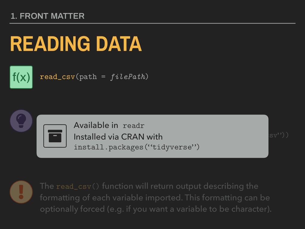
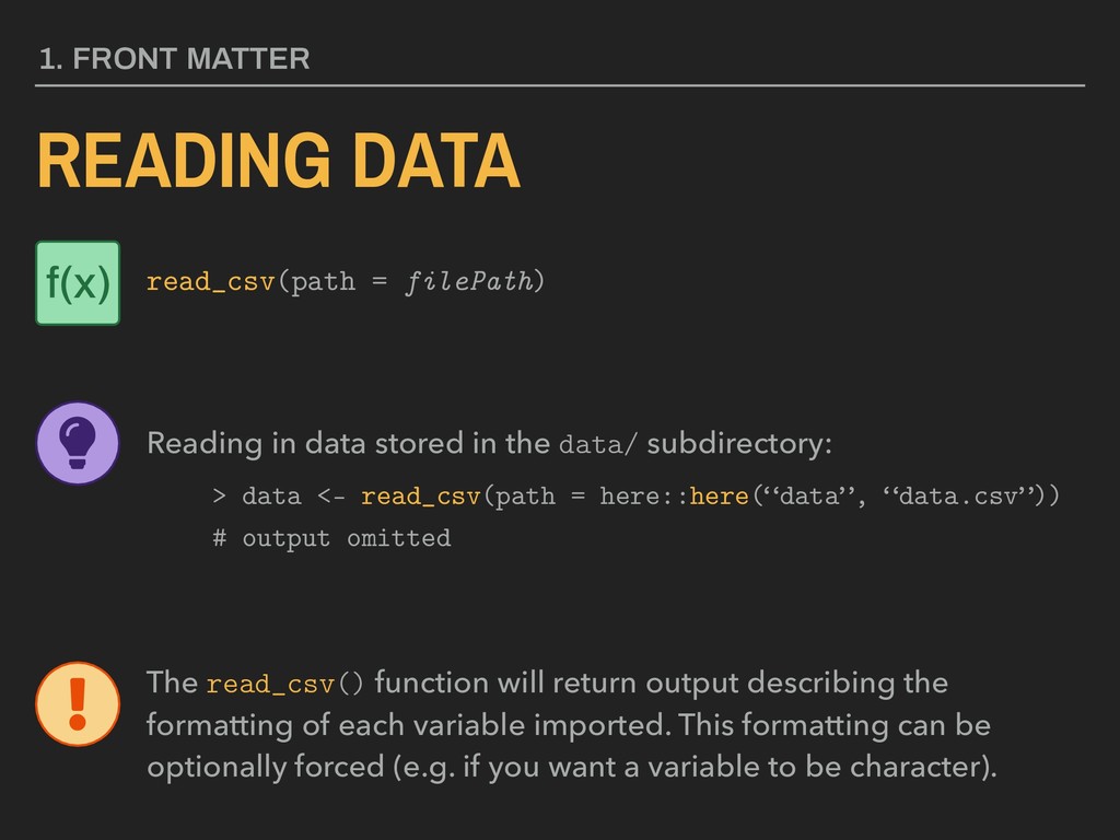
8. READING DATA 1. FRONT MATTER read_csv(path = filePath) Reading in data stored in the data/ subdirectory: > data <- read_csv(path = here::here(“data”, “data.csv”)) # output omitted The read_csv() function will return output describing the formatting of each variable imported. This formatting can be optionally forced (e.g. if you want a variable to be character). f(x) Available in readr
 Installed via CRAN with install.packages(“tidyverse”)
9. READING DATA 1. FRONT MATTER read_csv(path = filePath) Reading in data stored in the data/ subdirectory: > data <- read_csv(path = here::here(“data”, “data.csv”)) # output omitted The read_csv() function will return output describing the formatting of each variable imported. This formatting can be optionally forced (e.g. if you want a variable to be character). f(x)
10. PLOTS FOR MEAN DIFFERENCE 2
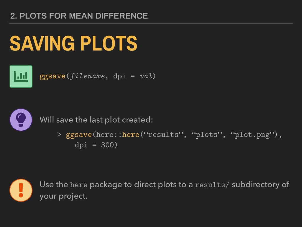
11. SAVING PLOTS 2. PLOTS FOR MEAN DIFFERENCE ggsave(filename, dpi = val) Will save the last plot created: > ggsave(here::here(“results”, “plots”, “plot.png”), 
 dpi = 300) Use the here package to direct plots to a results/ subdirectory of your project.
12. BOX PLOT
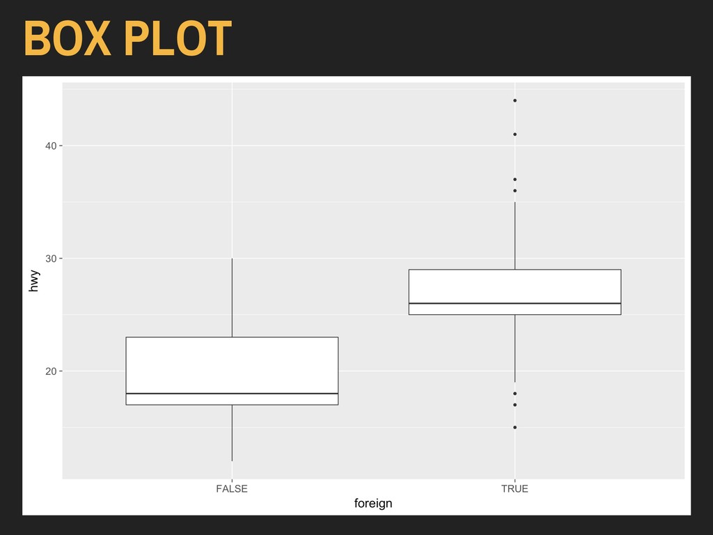
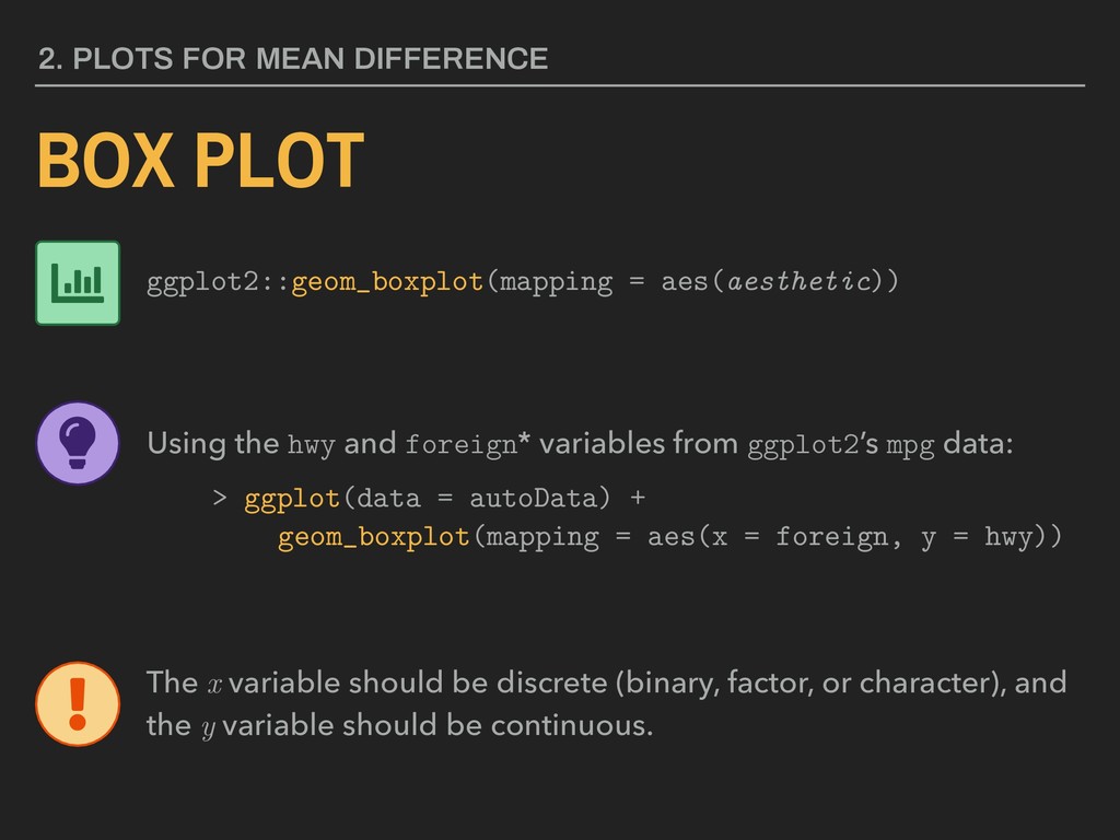
13. BOX PLOT 2. PLOTS FOR MEAN DIFFERENCE ggplot2::geom_boxplot(mapping = aes(aesthetic)) Using the hwy and foreign* variables from ggplot2’s mpg data: > ggplot(data = autoData) +
 geom_boxplot(mapping = aes(x = foreign, y = hwy)) The x variable should be discrete (binary, factor, or character), and the y variable should be continuous.
14. BOX PLOT 2. PLOTS FOR MEAN DIFFERENCE ggplot2::geom_boxplot(mapping = aes(aesthetic)) Using the hwy and foreign* variables from ggplot2’s mpg data: > ggplot(data = autoData) +
 geom_boxplot(mapping = aes(x = foreign, y = hwy)) Box plots are important parts of exploratory data analysis, but are less ideal for lay consumption.
15. BOX PLOT
16. VIOLIN PLOT
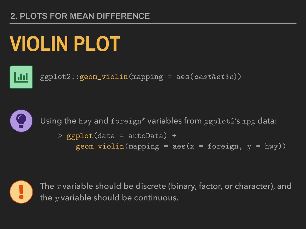
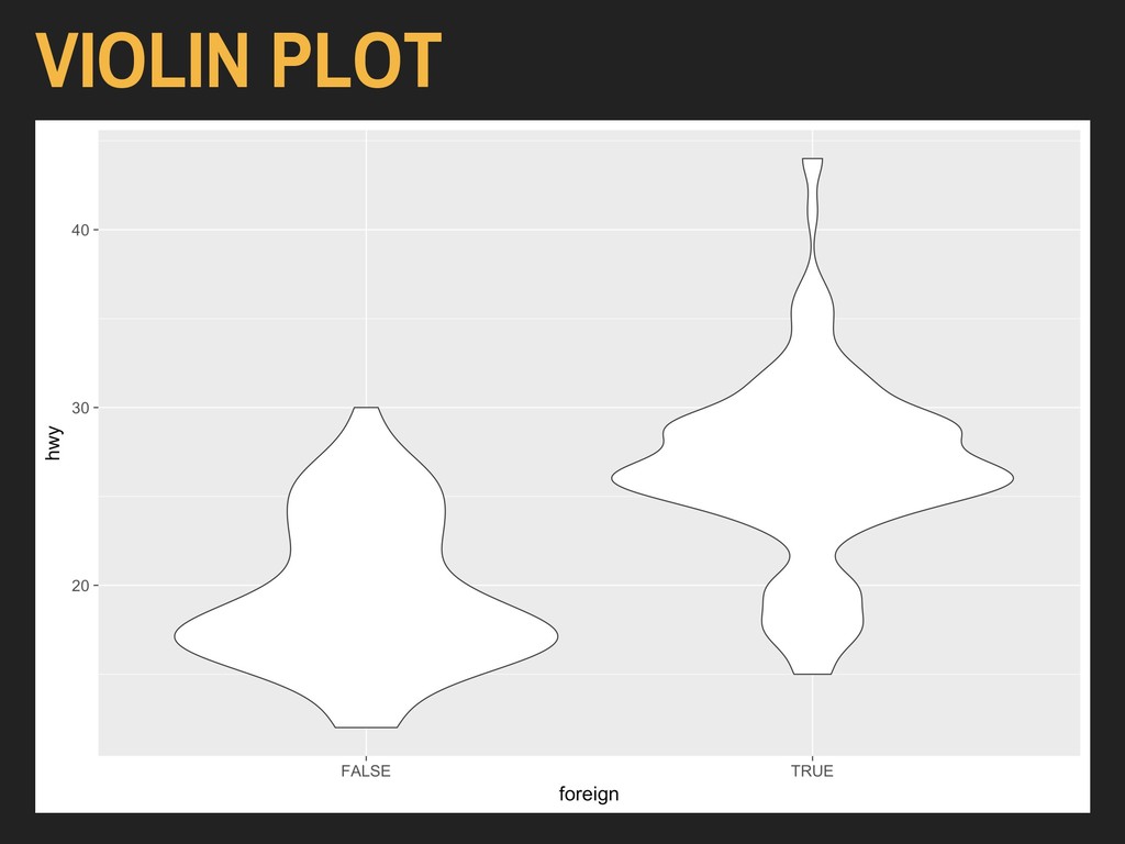
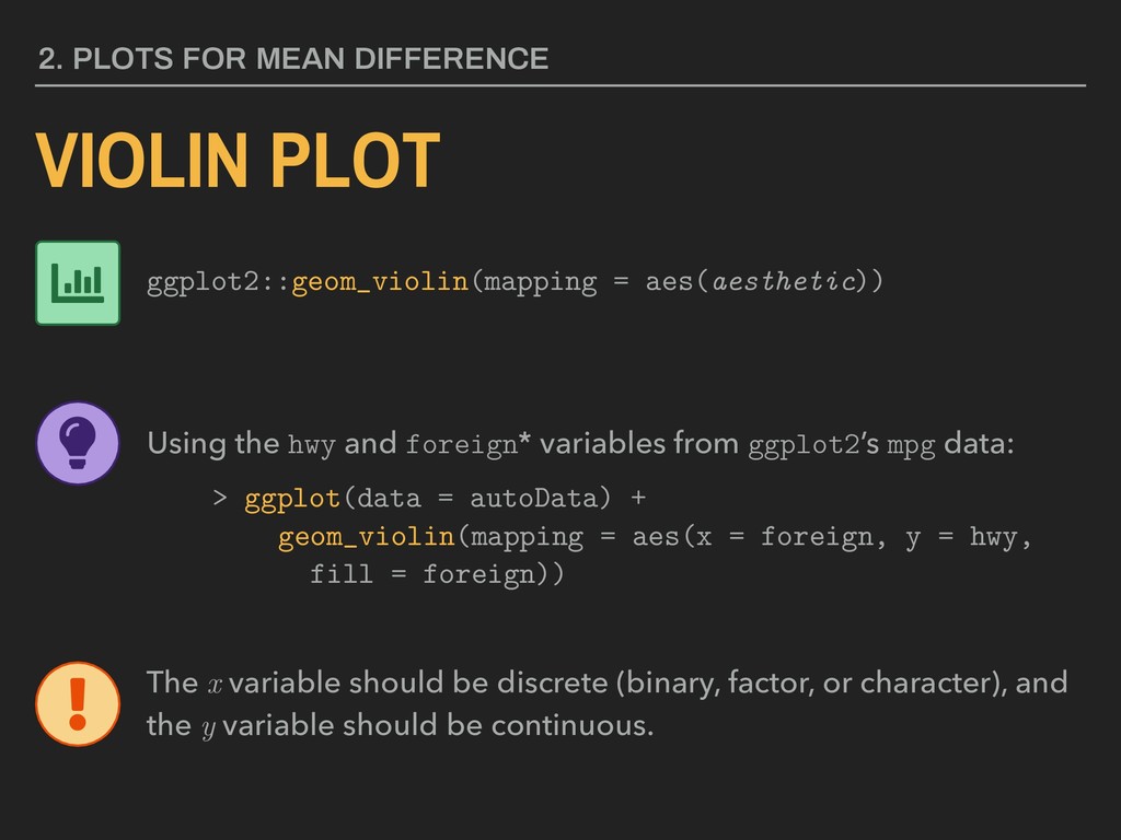
17. VIOLIN PLOT 2. PLOTS FOR MEAN DIFFERENCE ggplot2::geom_violin(mapping = aes(aesthetic)) Using the hwy and foreign* variables from ggplot2’s mpg data: > ggplot(data = autoData) +
 geom_violin(mapping = aes(x = foreign, y = hwy)) The x variable should be discrete (binary, factor, or character), and the y variable should be continuous.
18. VIOLIN PLOT
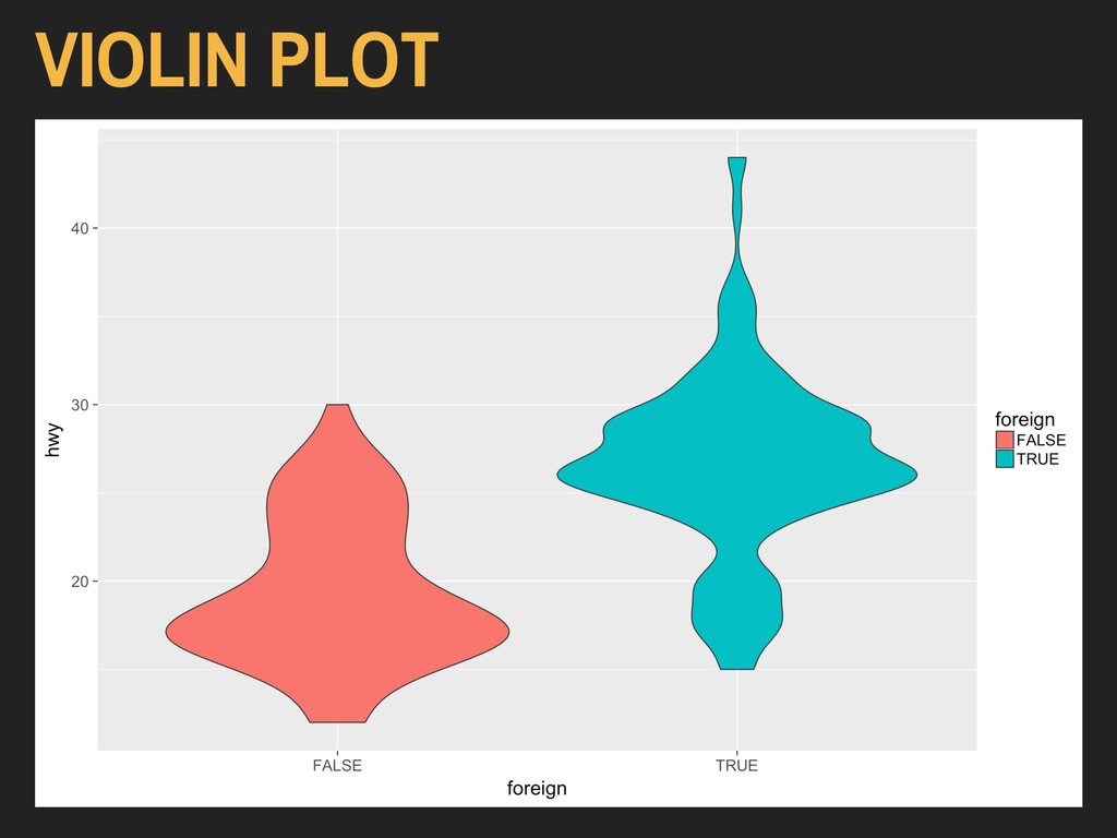
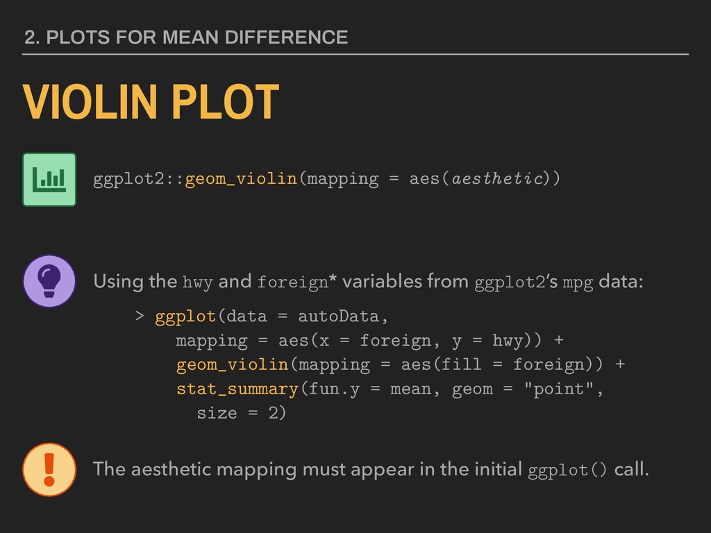
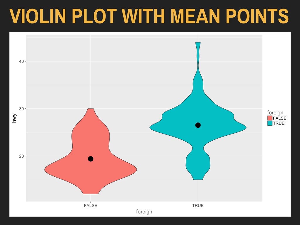
19. VIOLIN PLOT 2. PLOTS FOR MEAN DIFFERENCE ggplot2::geom_violin(mapping = aes(aesthetic)) Using the hwy and foreign* variables from ggplot2’s mpg data: > ggplot(data = autoData) +
 geom_violin(mapping = aes(x = foreign, y = hwy,
 fill = foreign)) The x variable should be discrete (binary, factor, or character), and the y variable should be continuous.
20. VIOLIN PLOT
21. VIOLIN PLOT 2. PLOTS FOR MEAN DIFFERENCE ggplot2::geom_violin(mapping = aes(aesthetic)) Using the hwy and foreign* variables from ggplot2’s mpg data: > ggplot(data = autoData, 
 mapping = aes(x = foreign, y = hwy)) +
 geom_violin(mapping = aes(fill = foreign)) +
 stat_summary(fun.y = mean, geom = "point", 
 size = 2) The aesthetic mapping must appear in the initial ggplot() call.
22. VIOLIN PLOT WITH MEAN POINTS
23. RIDGE PLOT
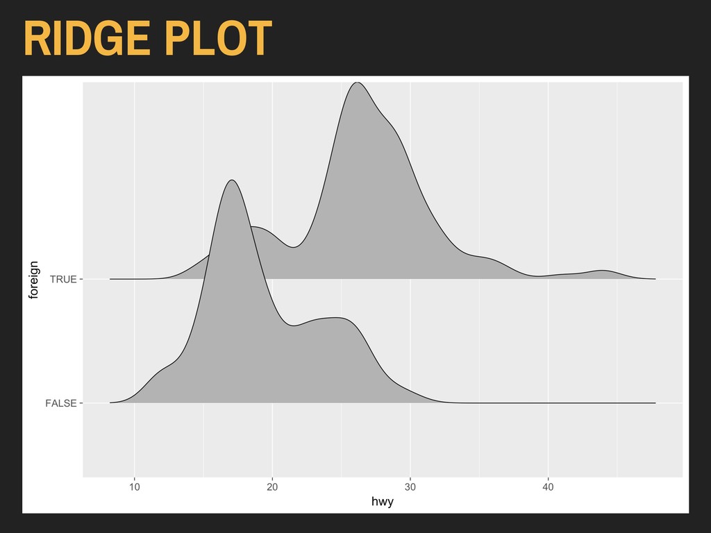
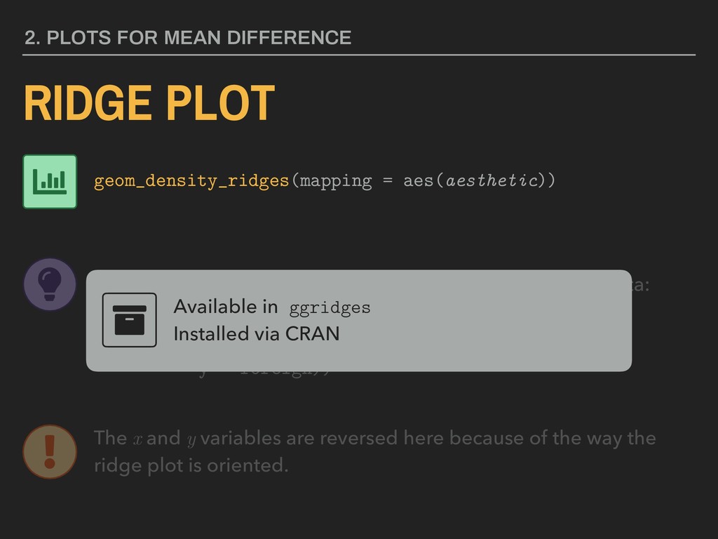
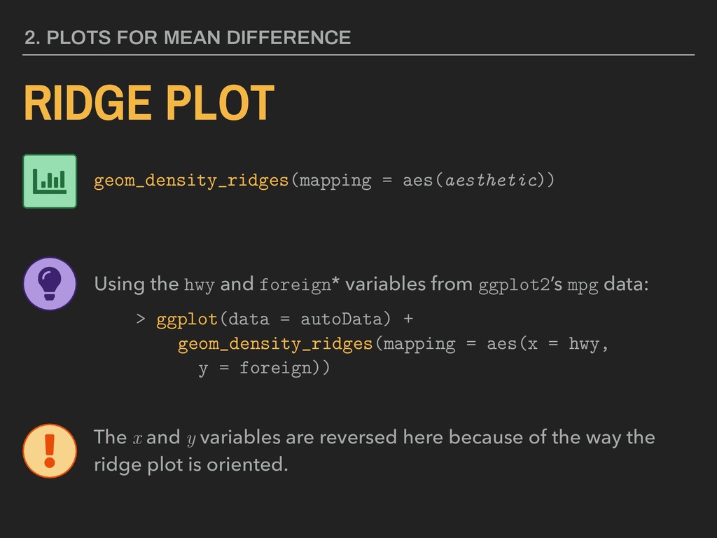
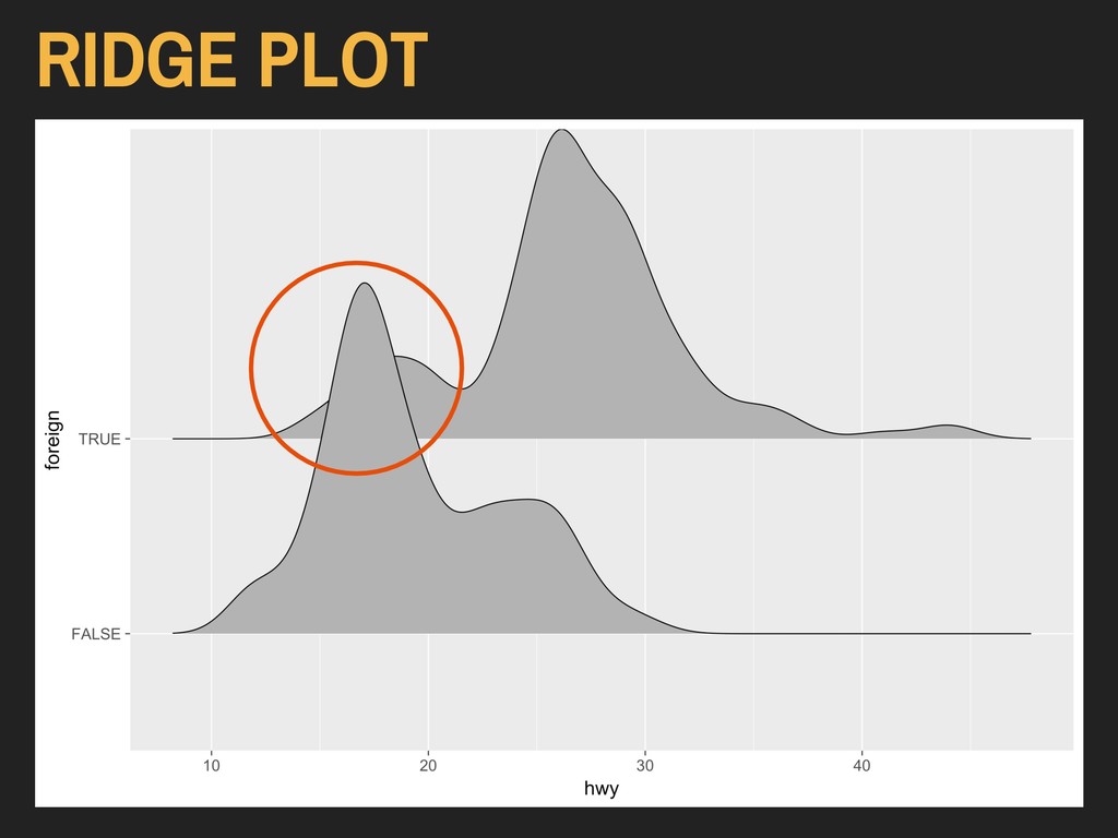
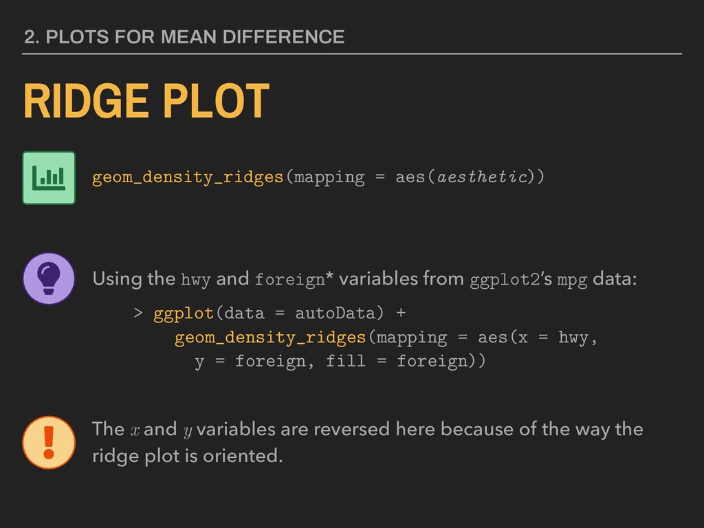
24. RIDGE PLOT 2. PLOTS FOR MEAN DIFFERENCE geom_density_ridges(mapping = aes(aesthetic)) Using the hwy and foreign* variables from ggplot2’s mpg data: > ggplot(data = autoData) +
 geom_density_ridges(mapping = aes(x = hwy, 
 y = foreign)) The x and y variables are reversed here because of the way the ridge plot is oriented. Available in ggridges
 Installed via CRAN
25. RIDGE PLOT 2. PLOTS FOR MEAN DIFFERENCE geom_density_ridges(mapping = aes(aesthetic)) Using the hwy and foreign* variables from ggplot2’s mpg data: > ggplot(data = autoData) +
 geom_density_ridges(mapping = aes(x = hwy, 
 y = foreign)) The x and y variables are reversed here because of the way the ridge plot is oriented.
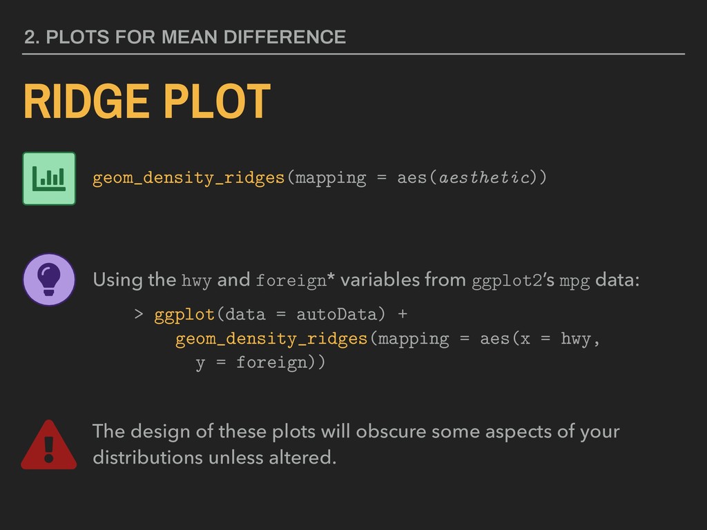
26. RIDGE PLOT 2. PLOTS FOR MEAN DIFFERENCE geom_density_ridges(mapping = aes(aesthetic)) Using the hwy and foreign* variables from ggplot2’s mpg data: > ggplot(data = autoData) +
 geom_density_ridges(mapping = aes(x = hwy, 
 y = foreign)) The design of these plots will obscure some aspects of your distributions unless altered.
27. RIDGE PLOT
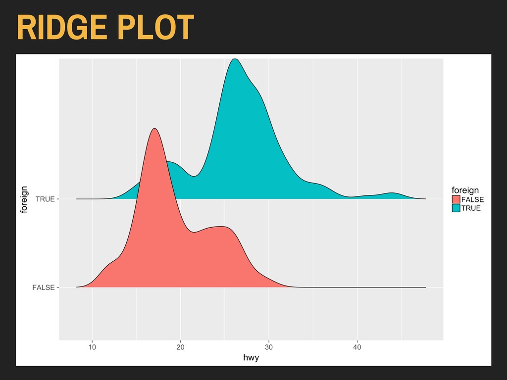
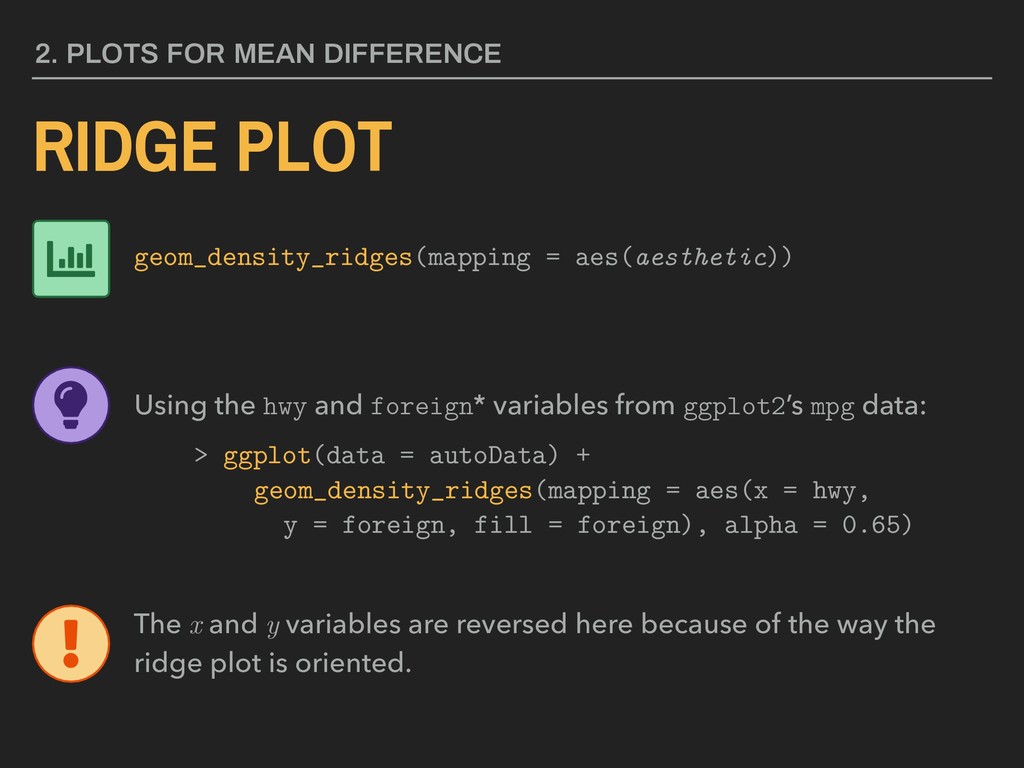
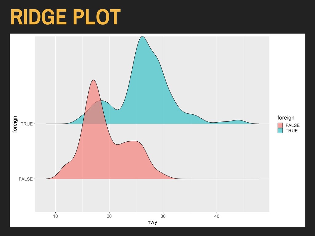
28. RIDGE PLOT 2. PLOTS FOR MEAN DIFFERENCE geom_density_ridges(mapping = aes(aesthetic)) Using the hwy and foreign* variables from ggplot2’s mpg data: > ggplot(data = autoData) +
 geom_density_ridges(mapping = aes(x = hwy, 
 y = foreign, fill = foreign)) The x and y variables are reversed here because of the way the ridge plot is oriented.
29. RIDGE PLOT
30. RIDGE PLOT
31. RIDGE PLOT 2. PLOTS FOR MEAN DIFFERENCE geom_density_ridges(mapping = aes(aesthetic)) Using the hwy and foreign* variables from ggplot2’s mpg data: > ggplot(data = autoData) +
 geom_density_ridges(mapping = aes(x = hwy, 
 y = foreign, fill = foreign), alpha = 0.65) The x and y variables are reversed here because of the way the ridge plot is oriented.
32. RIDGE PLOT
33. STATS PLOT
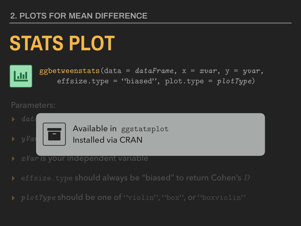
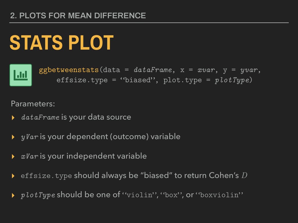
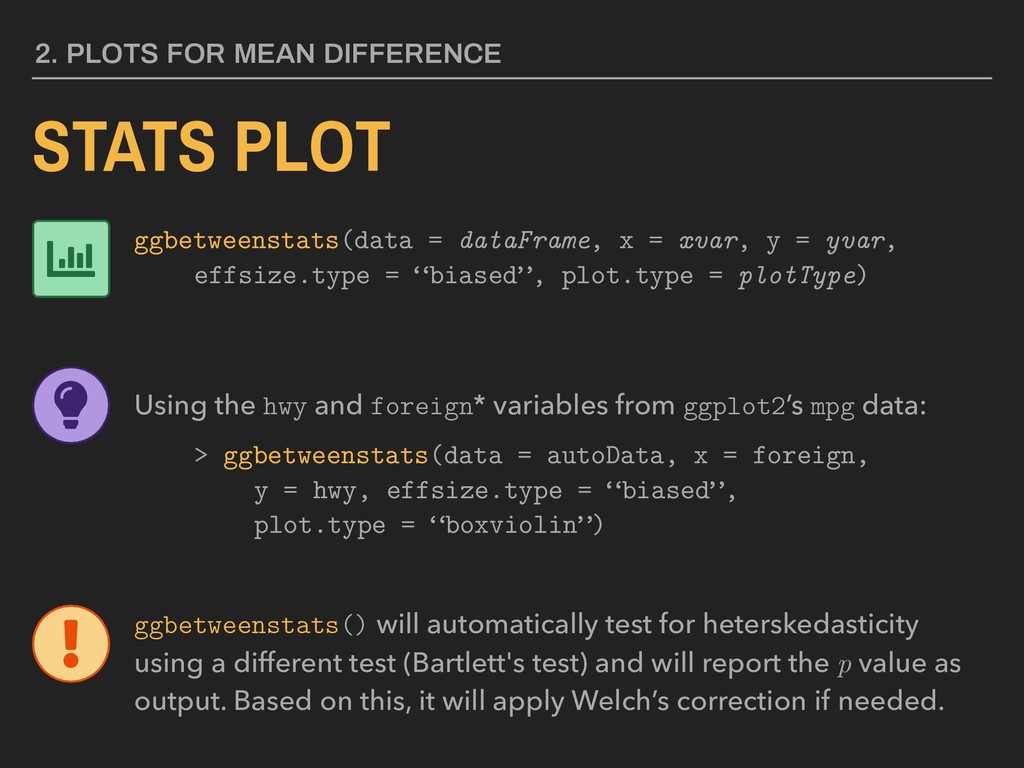
34. ▸ dataFrame is your data source ▸ yVar is your dependent (outcome) variable ▸ xVar is your independent variable ▸ effsize.type should always be “biased” to return Cohen’s D ▸ plotType should be one of “violin”, “box”, or “boxviolin” Available in ggstatsplot
 Installed via CRAN 2. PLOTS FOR MEAN DIFFERENCE STATS PLOT Parameters: ggbetweenstats(data = dataFrame, x = xvar, y = yvar,
 effsize.type = “biased”, plot.type = plotType)
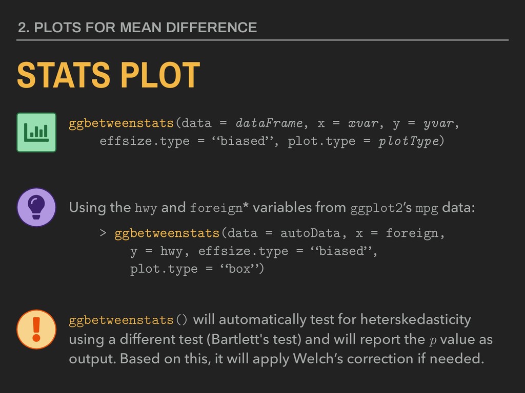
35. ▸ dataFrame is your data source ▸ yVar is your dependent (outcome) variable ▸ xVar is your independent variable ▸ effsize.type should always be “biased” to return Cohen’s D ▸ plotType should be one of “violin”, “box”, or “boxviolin” 2. PLOTS FOR MEAN DIFFERENCE STATS PLOT Parameters: ggbetweenstats(data = dataFrame, x = xvar, y = yvar,
 effsize.type = “biased”, plot.type = plotType)
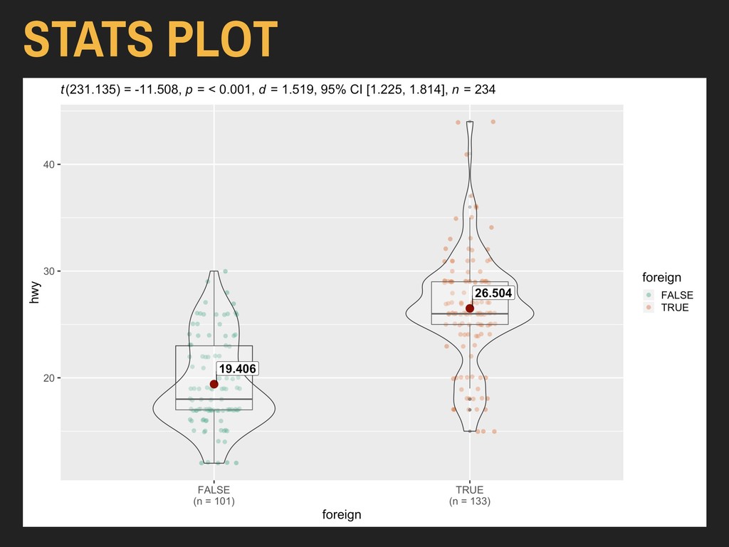
36. STATS PLOT 2. PLOTS FOR MEAN DIFFERENCE ggbetweenstats(data = dataFrame, x = xvar, y = yvar,
 effsize.type = “biased”, plot.type = plotType) Using the hwy and foreign* variables from ggplot2’s mpg data: > ggbetweenstats(data = autoData, x = foreign, 
 y = hwy, effsize.type = “biased”, 
 plot.type = “boxviolin”) ggbetweenstats() will automatically test for heterskedasticity using a different test (Bartlett's test) and will report the p value as output. Based on this, it will apply Welch’s correction if needed.
37. STATS PLOT
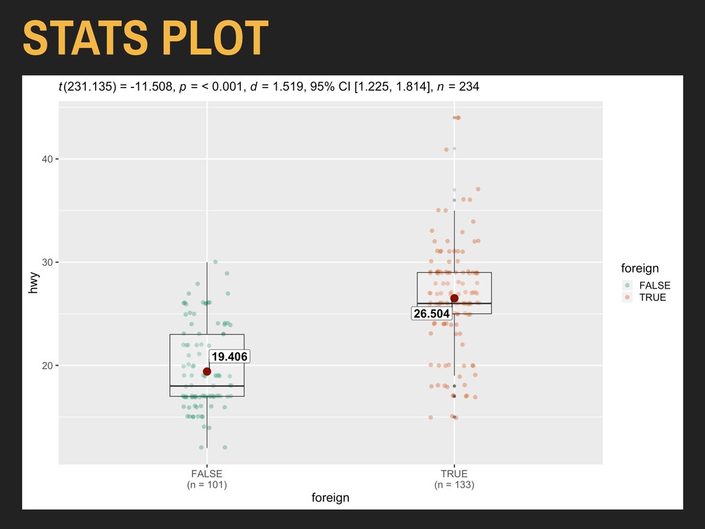
38. STATS PLOT 2. PLOTS FOR MEAN DIFFERENCE ggbetweenstats(data = dataFrame, x = xvar, y = yvar,
 effsize.type = “biased”, plot.type = plotType) Using the hwy and foreign* variables from ggplot2’s mpg data: > ggbetweenstats(data = autoData, x = foreign, 
 y = hwy, effsize.type = “biased”, 
 plot.type = “box”) ggbetweenstats() will automatically test for heterskedasticity using a different test (Bartlett's test) and will report the p value as output. Based on this, it will apply Welch’s correction if needed.
39. STATS PLOT
40. STATS PLOT 2. PLOTS FOR MEAN DIFFERENCE ggbetweenstats(data = dataFrame, x = xvar, y = yvar,
 effsize.type = “biased”, plot.type = plotType) Using the hwy and foreign* variables from ggplot2’s mpg data: > ggbetweenstats(data = autoData, x = foreign, 
 y = hwy, effsize.type = “biased”, 
 plot.type = “violin”) ggbetweenstats() will automatically test for heterskedasticity using a different test (Bartlett's test) and will report the p value as output. Based on this, it will apply Welch’s correction if needed.
41. STATS PLOT
42. VARIANCE TESTING 3
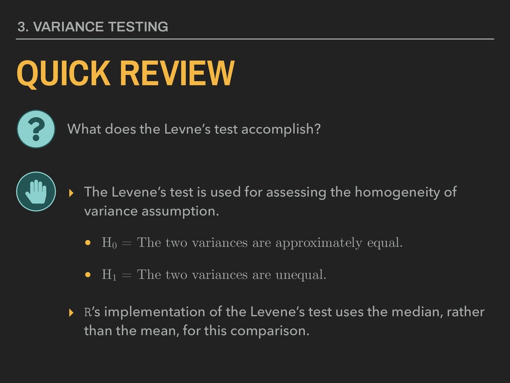
43. ? QUICK REVIEW ▸ The Levene’s test is used for assessing the homogeneity of variance assumption. • H0 = The two variances are approximately equal. • H1 = The two variances are unequal. ▸ R’s implementation of the Levene’s test uses the median, rather than the mean, for this comparison. 3. VARIANCE TESTING What does the Levne’s test accomplish?
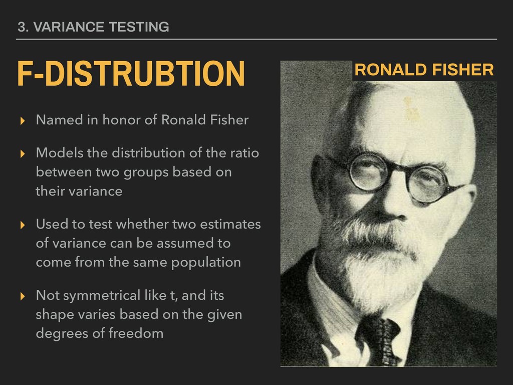
44. ▸ Named in honor of Ronald Fisher ▸ Models the distribution of the ratio between two groups based on their variance ▸ Used to test whether two estimates of variance can be assumed to come from the same population ▸ Not symmetrical like t, and its shape varies based on the given degrees of freedom 3. VARIANCE TESTING F-DISTRUBTION RONALD FISHER
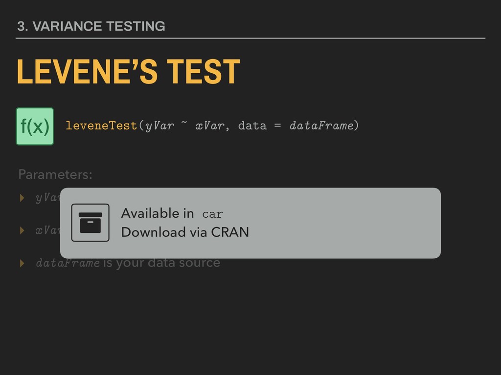
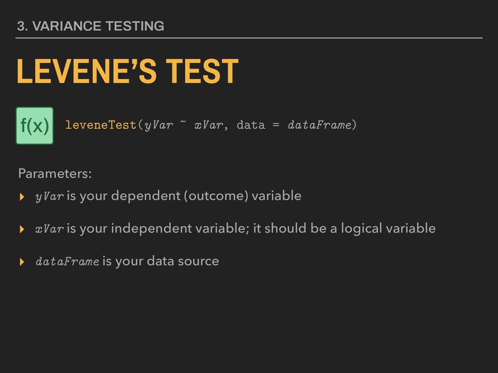
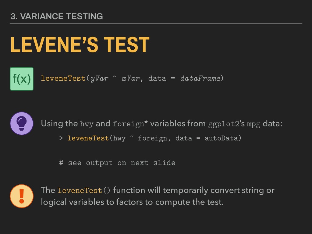
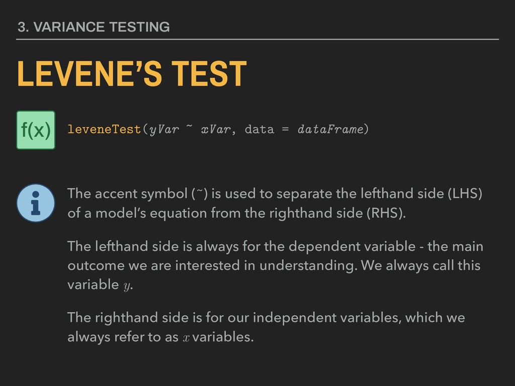
45. ▸ yVar is your dependent (outcome) variable ▸ xVar is your independent variable; it should be a logical variable ▸ dataFrame is your data source Available in car
 Download via CRAN 3. VARIANCE TESTING LEVENE’S TEST Parameters: leveneTest(yVar ~ xVar, data = dataFrame) f(x)
46. ▸ yVar is your dependent (outcome) variable ▸ xVar is your independent variable; it should be a logical variable ▸ dataFrame is your data source 3. VARIANCE TESTING LEVENE’S TEST Parameters: leveneTest(yVar ~ xVar, data = dataFrame) f(x)
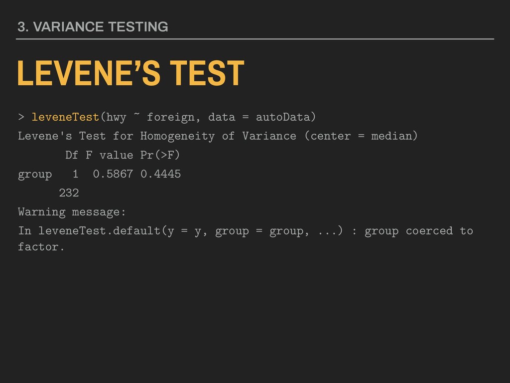
47. LEVENE’S TEST 3. VARIANCE TESTING leveneTest(yVar ~ xVar, data = dataFrame) Using the hwy and foreign* variables from ggplot2’s mpg data: > leveneTest(hwy ~ foreign, data = autoData) # see output on next slide The leveneTest() function will temporarily convert string or logical variables to factors to compute the test. f(x)
48. LEVENE’S TEST > leveneTest(hwy ~ foreign, data = autoData) Levene's Test for Homogeneity of Variance (center = median) Df F value Pr(>F) group 1 0.5867 0.4445 232 Warning message: In leveneTest.default(y = y, group = group, ...) : group coerced to factor. 3. VARIANCE TESTING
49. 3. VARIANCE TESTING LEVENE’S TEST 
 Report: 1. The value of f, the value of v, and the associated p value 2. A general statement - is the variance the same or different between xa and xb ?
50. 3. VARIANCE TESTING LEVENE’S TEST leveneTest(yVar ~ xVar, data = dataFrame) f(x) The accent symbol (~) is used to separate the lefthand side (LHS) of a model’s equation from the righthand side (RHS). The lefthand side is always for the dependent variable - the main outcome we are interested in understanding. We always call this variable y. The righthand side is for our independent variables, which we always refer to as x variables.
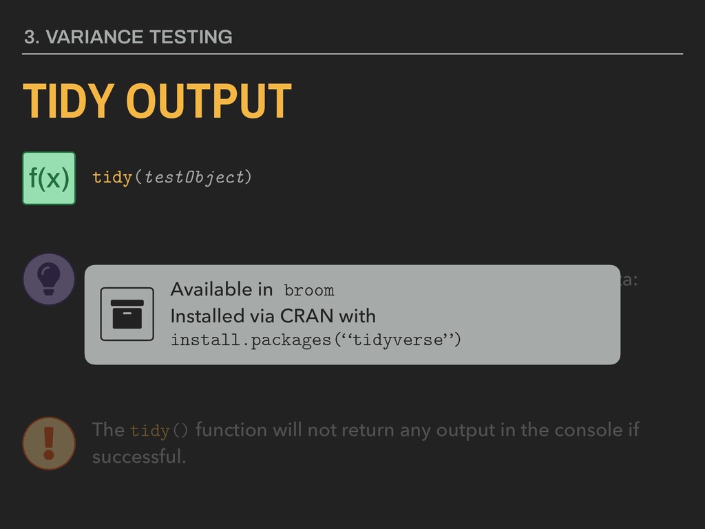
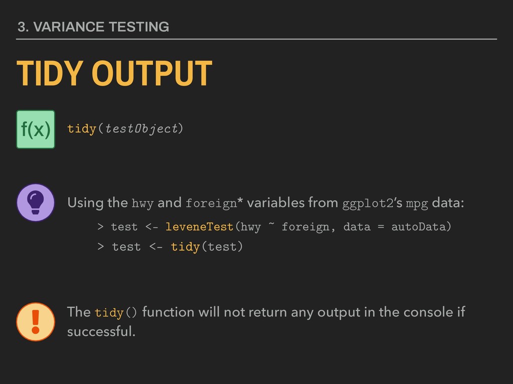
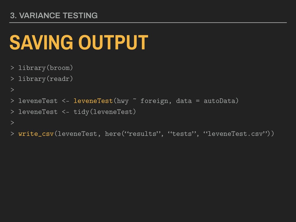
51. TIDY OUTPUT 3. VARIANCE TESTING tidy(testObject) Using the hwy and foreign* variables from ggplot2’s mpg data: > test <- leveneTest(hwy ~ foreign, data = autoData) > test <- tidy(test) The tidy() function will not return any output in the console if successful. f(x) Available in broom
 Installed via CRAN with install.packages(“tidyverse”)
52. TIDY OUTPUT 3. VARIANCE TESTING tidy(testObject) Using the hwy and foreign* variables from ggplot2’s mpg data: > test <- leveneTest(hwy ~ foreign, data = autoData) > test <- tidy(test) The tidy() function will not return any output in the console if successful. f(x)
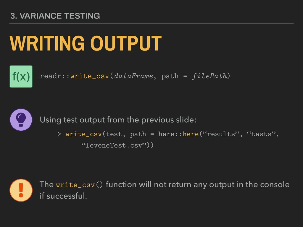
53. WRITING OUTPUT 3. VARIANCE TESTING readr::write_csv(dataFrame, path = filePath) Using test output from the previous slide: > write_csv(test, path = here::here(“results”, “tests”, “leveneTest.csv”)) The write_csv() function will not return any output in the console if successful. f(x)
54. SAVING OUTPUT > library(broom) > library(readr) > > leveneTest <- leveneTest(hwy ~ foreign, data = autoData) > leveneTest <- tidy(leveneTest) > > write_csv(leveneTest, here(“results”, “tests”, “leveneTest.csv”)) 3. VARIANCE TESTING
55. ONE OR TWO SAMPLES 4
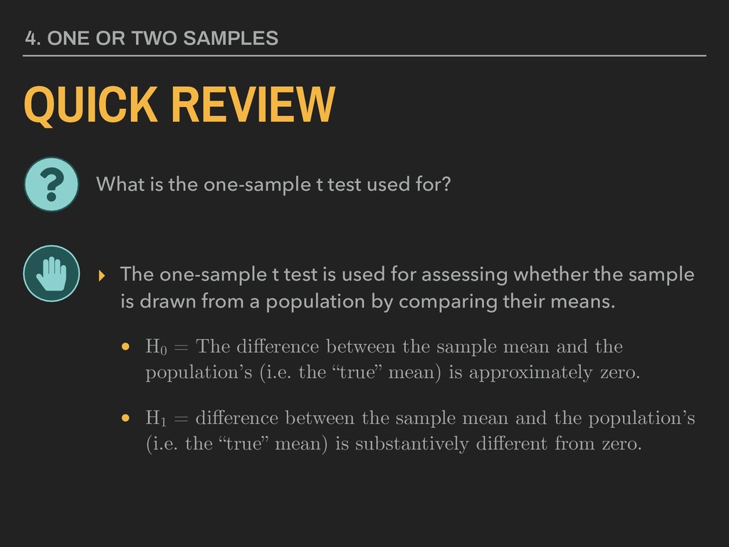
56. ? QUICK REVIEW ▸ The one-sample t test is used for assessing whether the sample is drawn from a population by comparing their means. • H0 = The difference between the sample mean and the population’s (i.e. the “true” mean) is approximately zero. • H1 = difference between the sample mean and the population’s (i.e. the “true” mean) is substantively different from zero. 4. ONE OR TWO SAMPLES What is the one-sample t test used for?
57. 4. ONE OR TWO SAMPLES ONE-SAMPLE T TEST 
 Assumptions: 1. The sample variable y contains continuous data 2. the distribution of y is approximately normal 3. Degrees of freedom (v) are defined as n-1
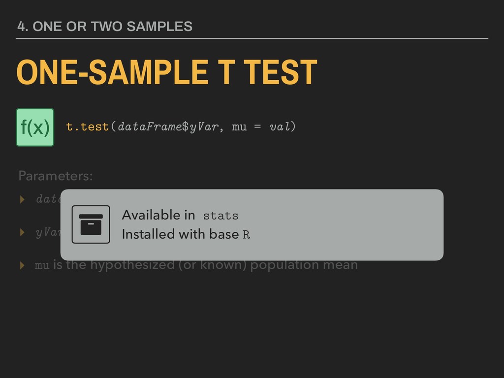
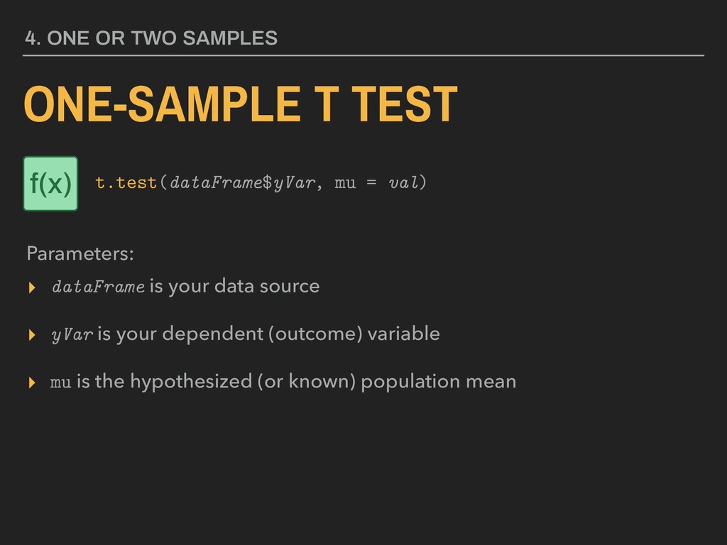
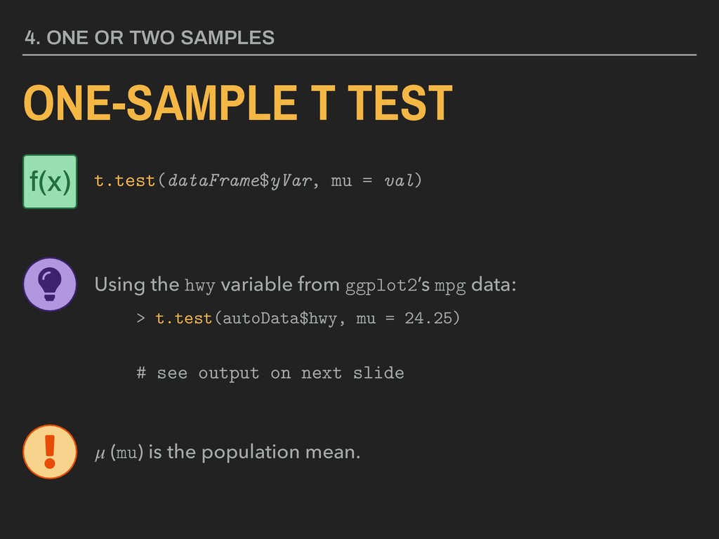
58. ▸ dataFrame is your data source ▸ yVar is your dependent (outcome) variable ▸ mu is the hypothesized (or known) population mean Available in stats
 Installed with base R 4. ONE OR TWO SAMPLES ONE-SAMPLE T TEST Parameters: t.test(dataFrame$yVar, mu = val) f(x)
59. ▸ dataFrame is your data source ▸ yVar is your dependent (outcome) variable ▸ mu is the hypothesized (or known) population mean 4. ONE OR TWO SAMPLES ONE-SAMPLE T TEST Parameters: t.test(dataFrame$yVar, mu = val) f(x)
60. ONE-SAMPLE T TEST 4. ONE OR TWO SAMPLES t.test(dataFrame$yVar, mu = val) Using the hwy variable from ggplot2’s mpg data: > t.test(autoData$hwy, mu = 24.25) # see output on next slide (mu) is the population mean. f(x)
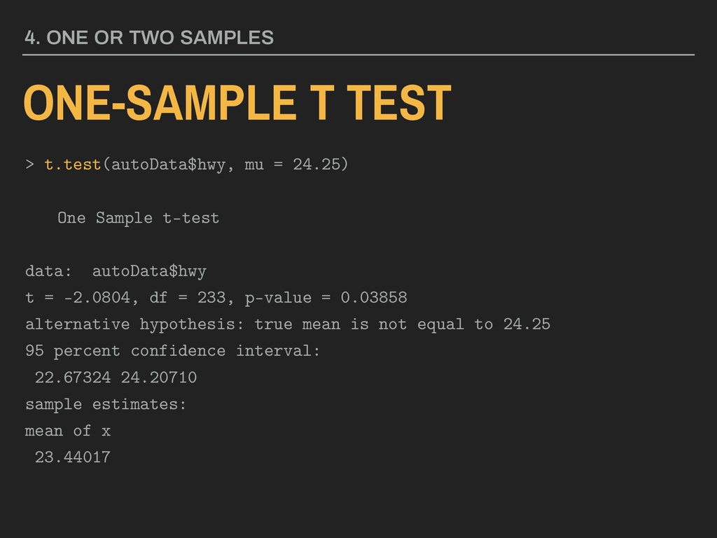
61. ONE-SAMPLE T TEST > t.test(autoData$hwy, mu = 24.25) One Sample t-test data: autoData$hwy t = -2.0804, df = 233, p-value = 0.03858 alternative hypothesis: true mean is not equal to 24.25 95 percent confidence interval: 22.67324 24.20710 sample estimates: mean of x 23.44017 4. ONE OR TWO SAMPLES
62. 4. ONE OR TWO SAMPLES ONE-SAMPLE T TEST 
 Report: 1. The value of t, the value of v, and the associated p value 2. A general statement - is the variance the same or different between y and ?
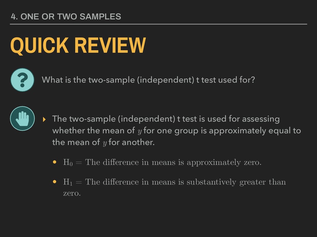
63. ? QUICK REVIEW ▸ The two-sample (independent) t test is used for assessing whether the mean of y for one group is approximately equal to the mean of y for another. • H0 = The difference in means is approximately zero. • H1 = The difference in means is substantively greater than zero. 4. ONE OR TWO SAMPLES What is the two-sample (independent) t test used for?
64. 4. ONE OR TWO SAMPLES INDEPENDENT SAMPLES T-TEST 
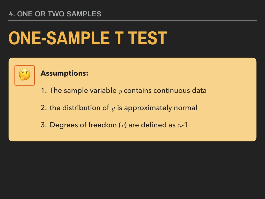
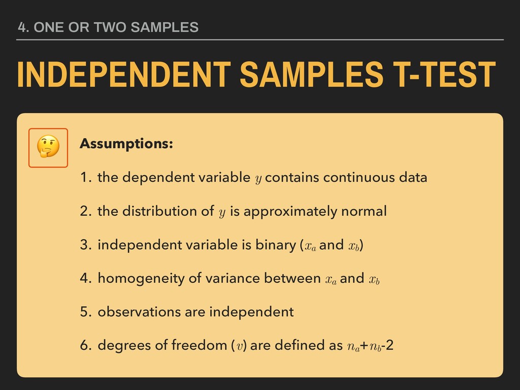
 Assumptions: 1. the dependent variable y contains continuous data 2. the distribution of y is approximately normal 3. independent variable is binary (xa and xb ) 4. homogeneity of variance between xa and xb 5. observations are independent 6. degrees of freedom (v) are defined as na +nb -2
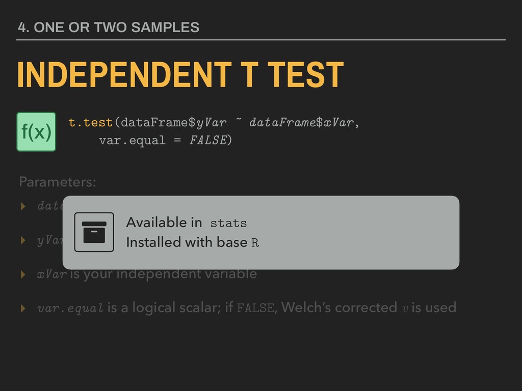
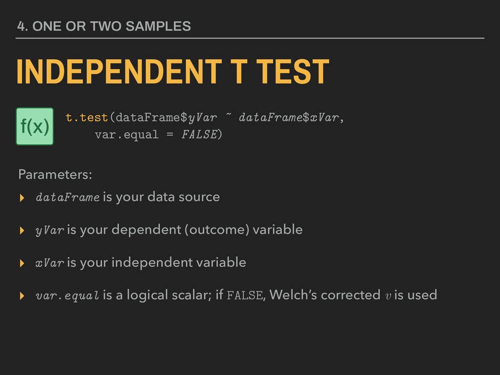
65. ▸ dataFrame is your data source ▸ yVar is your dependent (outcome) variable ▸ xVar is your independent variable ▸ var.equal is a logical scalar; if FALSE, Welch’s corrected v is used Available in stats
 Installed with base R 4. ONE OR TWO SAMPLES INDEPENDENT T TEST Parameters: t.test(dataFrame$yVar ~ dataFrame$xVar, 
 var.equal = FALSE) f(x)
66. ▸ dataFrame is your data source ▸ yVar is your dependent (outcome) variable ▸ xVar is your independent variable ▸ var.equal is a logical scalar; if FALSE, Welch’s corrected v is used 4. ONE OR TWO SAMPLES INDEPENDENT T TEST Parameters: t.test(dataFrame$yVar ~ dataFrame$xVar, 
 var.equal = FALSE) f(x)
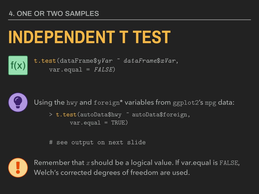
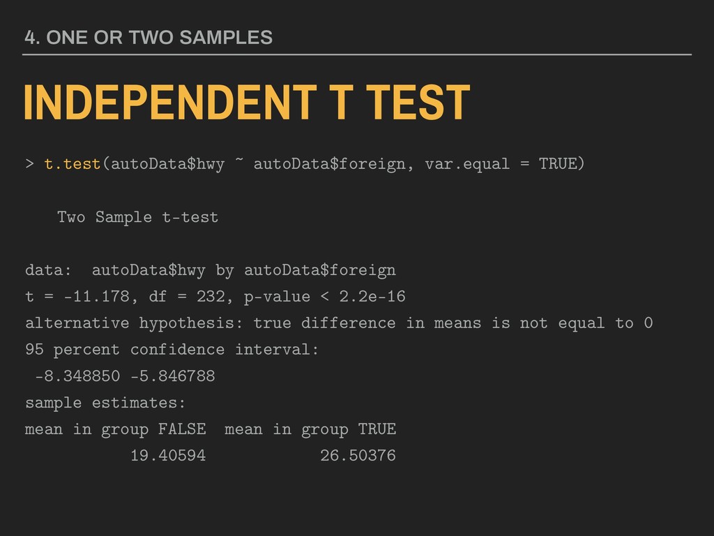
67. INDEPENDENT T TEST 4. ONE OR TWO SAMPLES t.test(dataFrame$yVar ~ dataFrame$xVar, 
 var.equal = FALSE) Using the hwy and foreign* variables from ggplot2’s mpg data: > t.test(autoData$hwy ~ autoData$foreign, 
 var.equal = TRUE) # see output on next slide Remember that x should be a logical value. If var.equal is FALSE, Welch’s corrected degrees of freedom are used. f(x)
68. INDEPENDENT T TEST > t.test(autoData$hwy ~ autoData$foreign, var.equal = TRUE) Two Sample t-test data: autoData$hwy by autoData$foreign t = -11.178, df = 232, p-value < 2.2e-16 alternative hypothesis: true difference in means is not equal to 0 95 percent confidence interval: -8.348850 -5.846788 sample estimates: mean in group FALSE mean in group TRUE 19.40594 26.50376 4. ONE OR TWO SAMPLES
69. 4. ONE OR TWO SAMPLES INDEPENDENT T TEST 
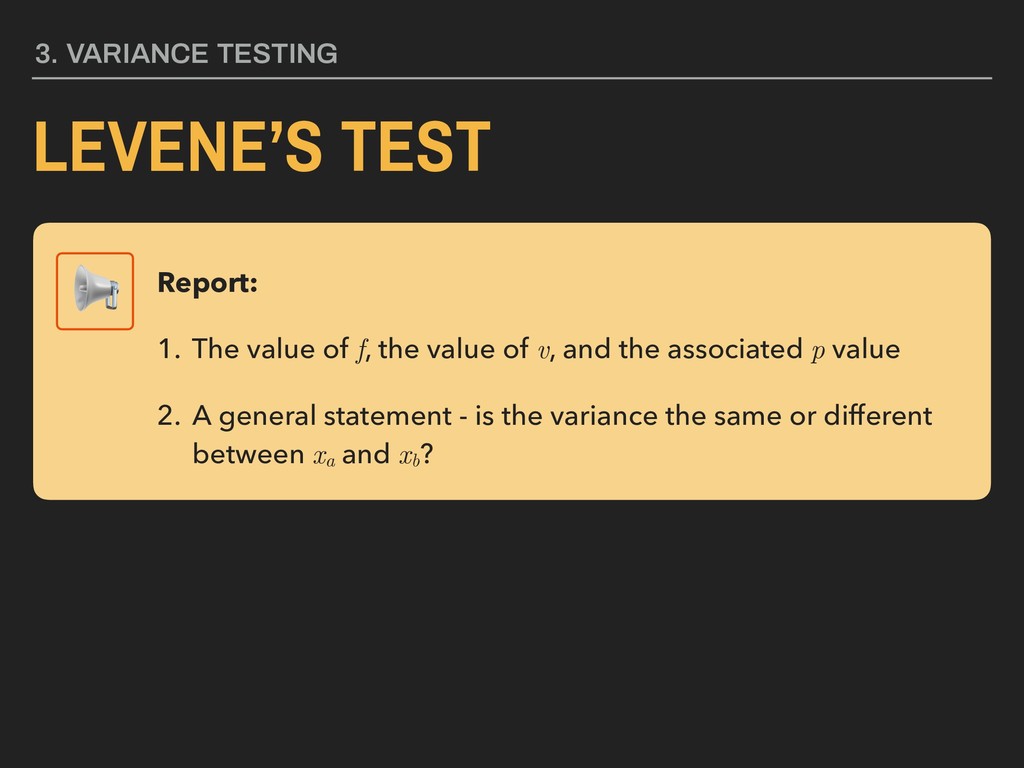
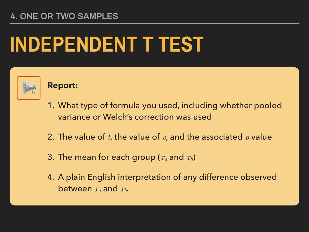
 Report: 1. What type of formula you used, including whether pooled variance or Welch’s correction was used 2. The value of t, the value of v, and the associated p value 3. The mean for each group (xa and xb ) 4. A plain English interpretation of any difference observed between xa and xb .
70. DEPENDENT SAMPLES 5
71. EXAMPLE DATA > income <- read_csv(here(“data”, “stl_tbl_income”)) > income # A tibble: 106 x 10 geoID tractCE nameLSAD variable mi10 mi10_moe mi10_inflate mi16 mi16_moe delta <chr> <int> <chr> <chr> <dbl> <dbl> <dbl> <dbl> <dbl> <dbl> 1 29510101100 101100 Census Tract 1011… B19013_001 45530 9265 50477. 56506 9046 6029. 2 29510101200 101200 Census Tract 1012… B19013_001 58684 9715 65060. 54828 9400 -10232. 3 29510101300 101300 Census Tract 1013… B19013_001 44403 6734 49227. 54775 9721 5548. 4 29510101400 101400 Census Tract 1014… B19013_001 40100 9341 44457. 39671 4303 -4786. 5 29510101500 101500 Census Tract 1015… B19013_001 30266 5736 33554. 28689 3526 -4865. 6 29510101800 101800 Census Tract 1018… B19013_001 27439 5485 30420. 38333 6589 7913. 7 29510102100 102100 Census Tract 1021… B19013_001 35475 2864 39329. 45230 5949 5901. 8 29510102200 102200 Census Tract 1022… B19013_001 57303 3319 63529. 68537 12085 5008. 9 29510102300 102300 Census Tract 1023… B19013_001 53277 10920 59065. 54583 8097 -4482. 10 29510102400 102400 Census Tract 1024… B19013_001 39191 7145 43449. 38676 5550 -4773. # ... with 96 more rows 5. DEPENDENT SAMPLES
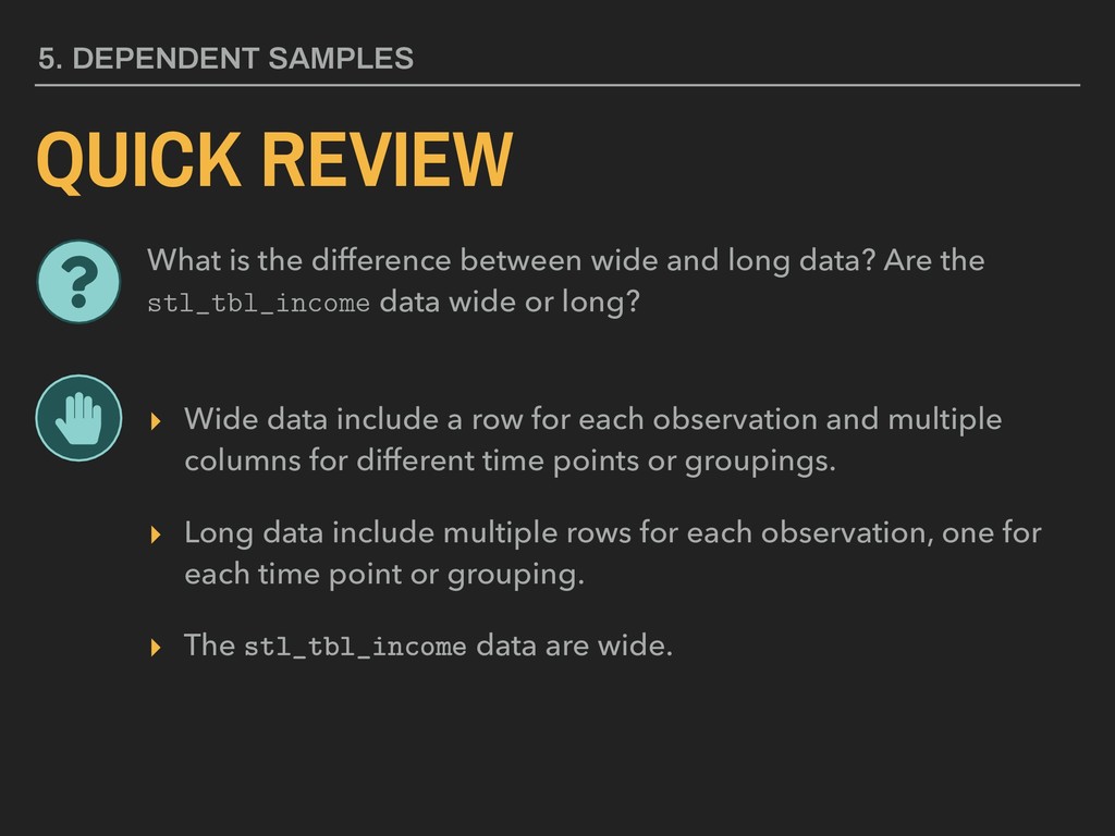
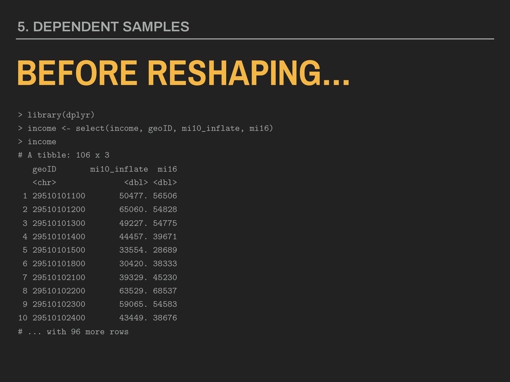
72. ? QUICK REVIEW ▸ Wide data include a row for each observation and multiple columns for different time points or groupings. ▸ Long data include multiple rows for each observation, one for each time point or grouping. ▸ The stl_tbl_income data are wide. 5. DEPENDENT SAMPLES What is the difference between wide and long data? Are the stl_tbl_income data wide or long?
73. BEFORE RESHAPING… > library(dplyr) > income <- select(income, geoID, mi10_inflate, mi16) > income # A tibble: 106 x 3 geoID mi10_inflate mi16 <chr> <dbl> <dbl> 1 29510101100 50477. 56506 2 29510101200 65060. 54828 3 29510101300 49227. 54775 4 29510101400 44457. 39671 5 29510101500 33554. 28689 6 29510101800 30420. 38333 7 29510102100 39329. 45230 8 29510102200 63529. 68537 9 29510102300 59065. 54583 10 29510102400 43449. 38676 # ... with 96 more rows 5. DEPENDENT SAMPLES
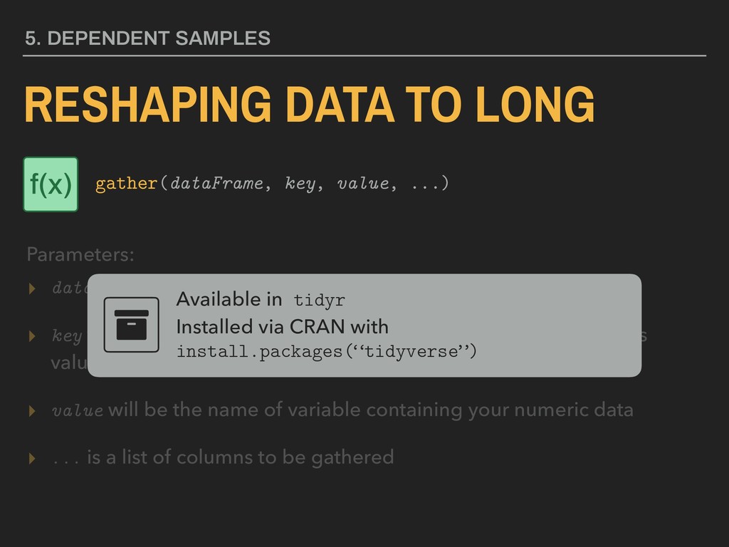
74. ▸ dataFrame is your data source ▸ key will be the name of your new identification variable that takes values from the gathered columns’ names ▸ value will be the name of variable containing your numeric data ▸ ... is a list of columns to be gathered Available in tidyr
 Installed via CRAN with install.packages(“tidyverse”) 5. DEPENDENT SAMPLES RESHAPING DATA TO LONG Parameters: gather(dataFrame, key, value, ...) f(x)
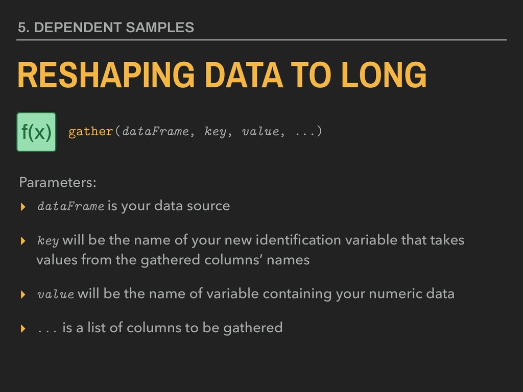
75. ▸ dataFrame is your data source ▸ key will be the name of your new identification variable that takes values from the gathered columns’ names ▸ value will be the name of variable containing your numeric data ▸ ... is a list of columns to be gathered 5. DEPENDENT SAMPLES RESHAPING DATA TO LONG Parameters: gather(dataFrame, key, value, ...) f(x)
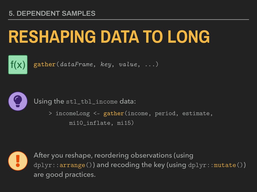
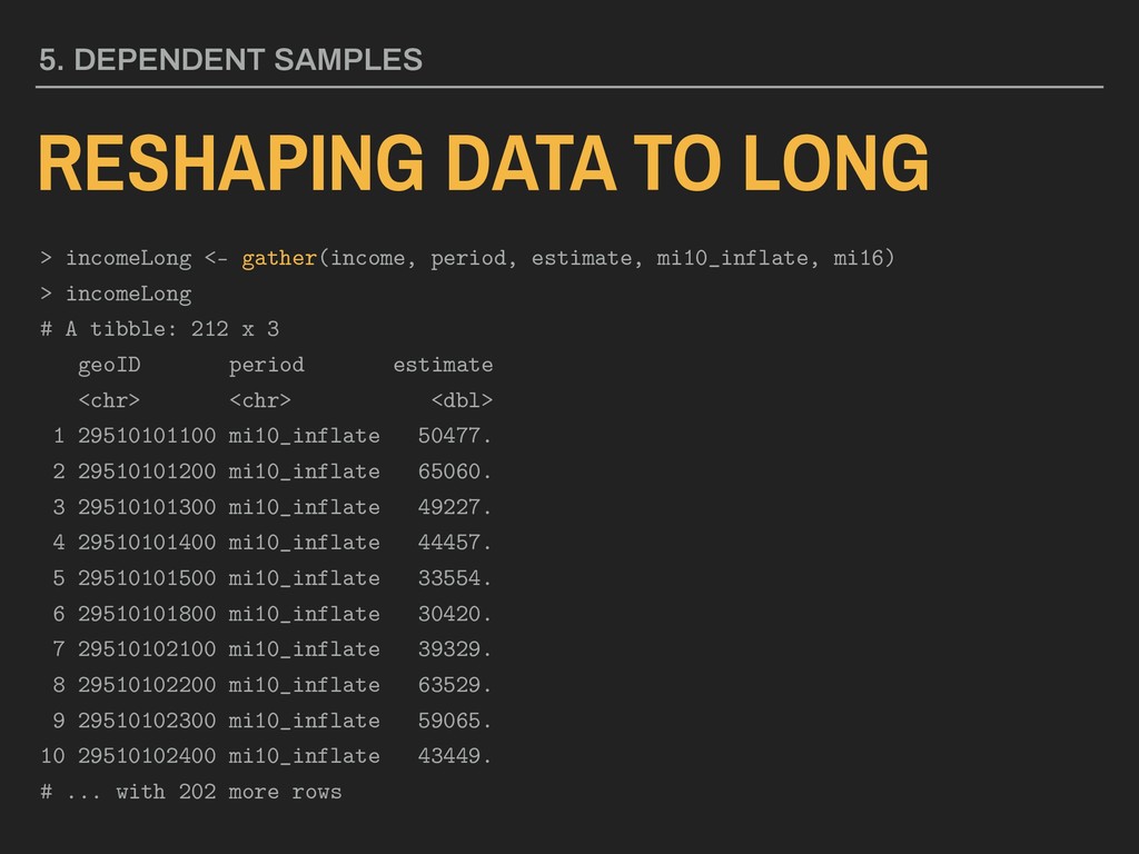
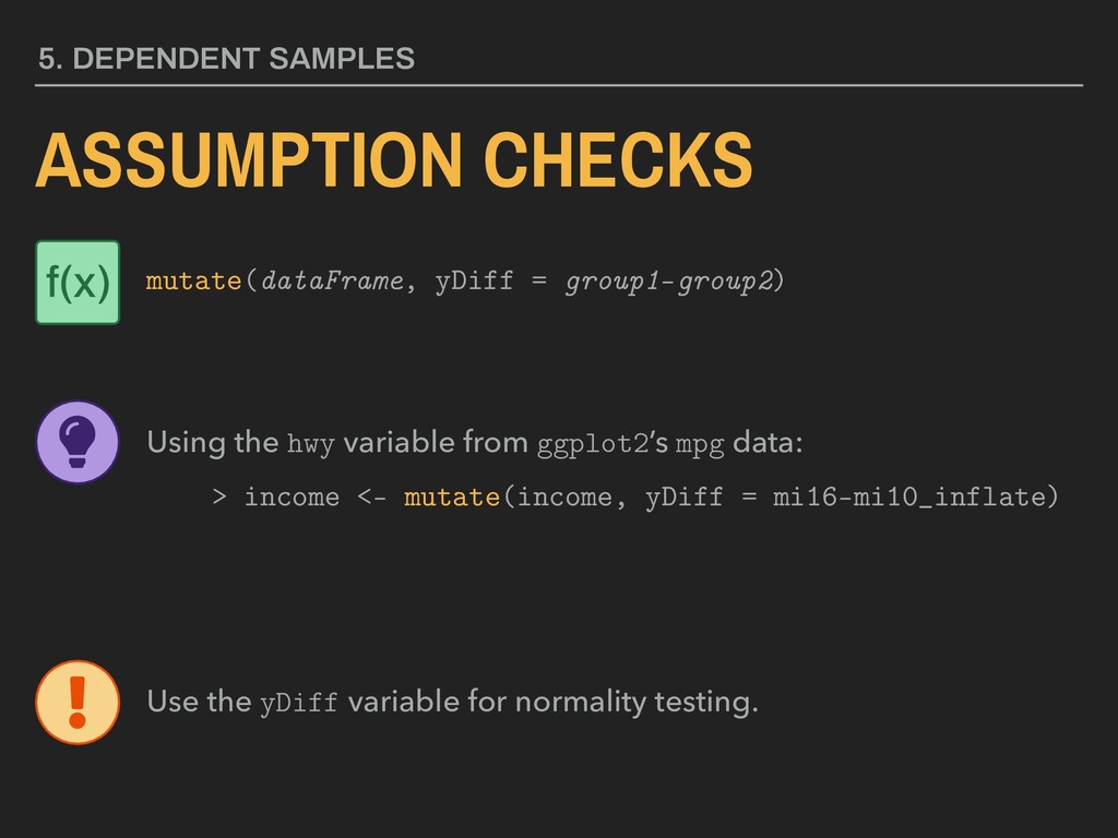
76. RESHAPING DATA TO LONG 5. DEPENDENT SAMPLES gather(dataFrame, key, value, ...) Using the stl_tbl_income data: > incomeLong <- gather(income, period, estimate, mi10_inflate, mi15) After you reshape, reordering observations (using dplyr::arrange()) and recoding the key (using dplyr::mutate()) are good practices. f(x)
77. RESHAPING DATA TO LONG > incomeLong <- gather(income, period, estimate, mi10_inflate, mi16) > incomeLong # A tibble: 212 x 3 geoID period estimate <chr> <chr> <dbl> 1 29510101100 mi10_inflate 50477. 2 29510101200 mi10_inflate 65060. 3 29510101300 mi10_inflate 49227. 4 29510101400 mi10_inflate 44457. 5 29510101500 mi10_inflate 33554. 6 29510101800 mi10_inflate 30420. 7 29510102100 mi10_inflate 39329. 8 29510102200 mi10_inflate 63529. 9 29510102300 mi10_inflate 59065. 10 29510102400 mi10_inflate 43449. # ... with 202 more rows 5. DEPENDENT SAMPLES
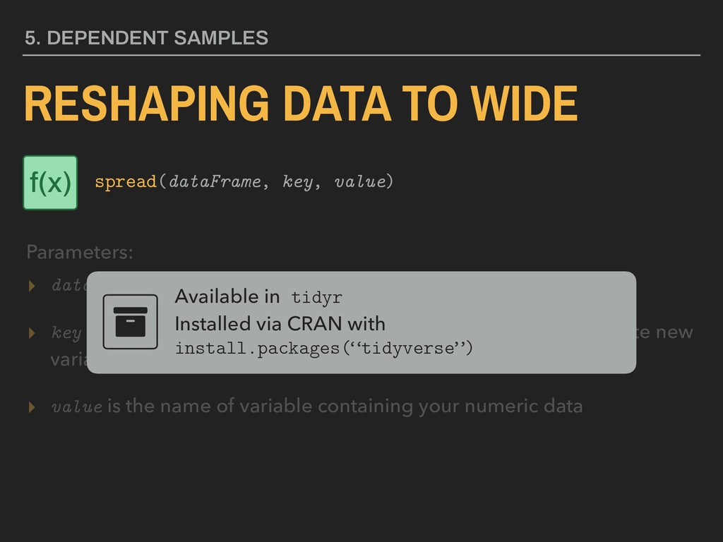
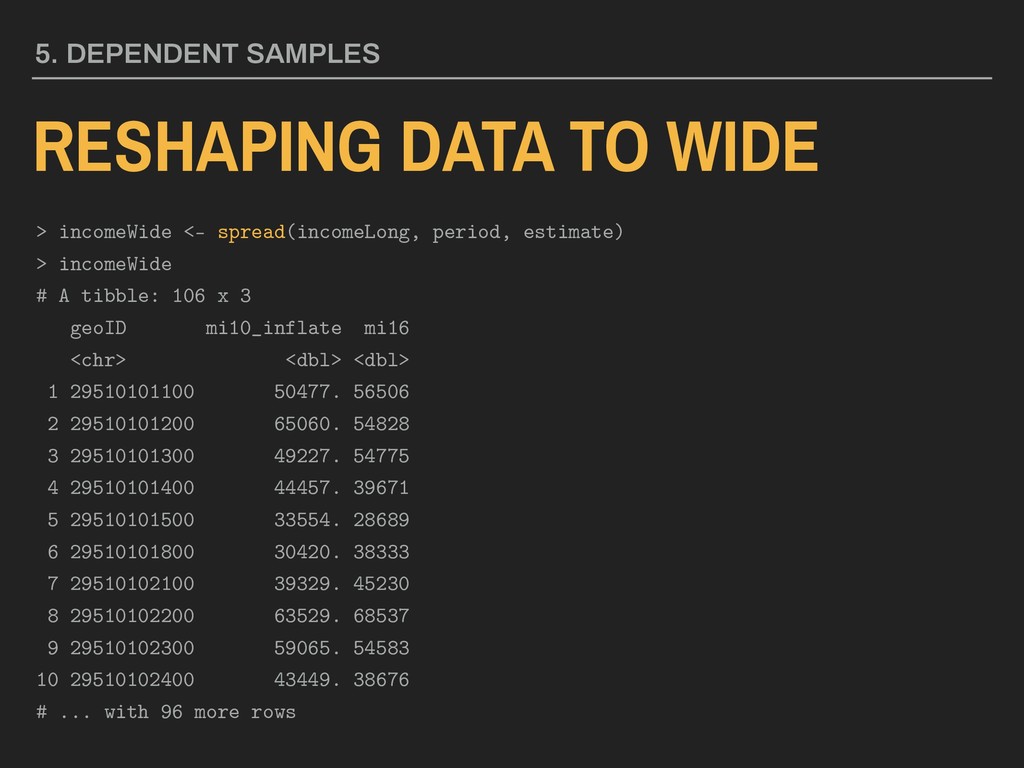
78. ▸ dataFrame is your data source ▸ key is the name of the variable whose values will be used to create new variable names ▸ value is the name of variable containing your numeric data Available in tidyr
 Installed via CRAN with install.packages(“tidyverse”) 5. DEPENDENT SAMPLES RESHAPING DATA TO WIDE Parameters: spread(dataFrame, key, value) f(x)
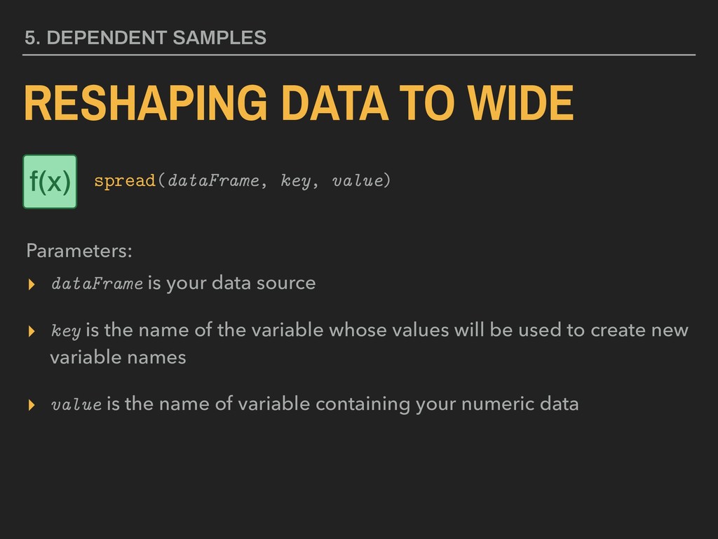
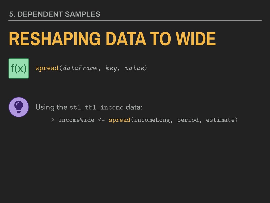
79. ▸ dataFrame is your data source ▸ key is the name of the variable whose values will be used to create new variable names ▸ value is the name of variable containing your numeric data 5. DEPENDENT SAMPLES RESHAPING DATA TO WIDE Parameters: spread(dataFrame, key, value) f(x)
80. RESHAPING DATA TO WIDE 5. DEPENDENT SAMPLES spread(dataFrame, key, value) Using the stl_tbl_income data: > incomeWide <- spread(incomeLong, period, estimate) f(x)
81. RESHAPING DATA TO WIDE > incomeWide <- spread(incomeLong, period, estimate) > incomeWide # A tibble: 106 x 3 geoID mi10_inflate mi16 <chr> <dbl> <dbl> 1 29510101100 50477. 56506 2 29510101200 65060. 54828 3 29510101300 49227. 54775 4 29510101400 44457. 39671 5 29510101500 33554. 28689 6 29510101800 30420. 38333 7 29510102100 39329. 45230 8 29510102200 63529. 68537 9 29510102300 59065. 54583 10 29510102400 43449. 38676 # ... with 96 more rows 5. DEPENDENT SAMPLES
82. Plots from ggplot2 require long data. The t.test() function requires wide data. f(x) WHAT TO USE WHEN 5. DEPENDENT SAMPLES
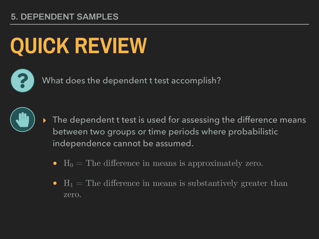
83. ? QUICK REVIEW ▸ The dependent t test is used for assessing the difference means between two groups or time periods where probabilistic independence cannot be assumed. • H0 = The difference in means is approximately zero. • H1 = The difference in means is substantively greater than zero. 5. DEPENDENT SAMPLES What does the dependent t test accomplish?
84. 5. DEPENDENT SAMPLES DEPENDENT SAMPLES T-TEST 
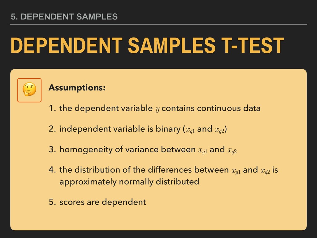
 Assumptions: 1. the dependent variable y contains continuous data 2. independent variable is binary (xg1 and xg2 ) 3. homogeneity of variance between xg1 and xg2 4. the distribution of the differences between xg1 and xg2 is approximately normally distributed 5. scores are dependent
85. ASSUMPTION CHECKS 5. DEPENDENT SAMPLES mutate(dataFrame, yDiff = group1-group2) Using the hwy variable from ggplot2’s mpg data: > income <- mutate(income, yDiff = mi16-mi10_inflate) Use the yDiff variable for normality testing. f(x)
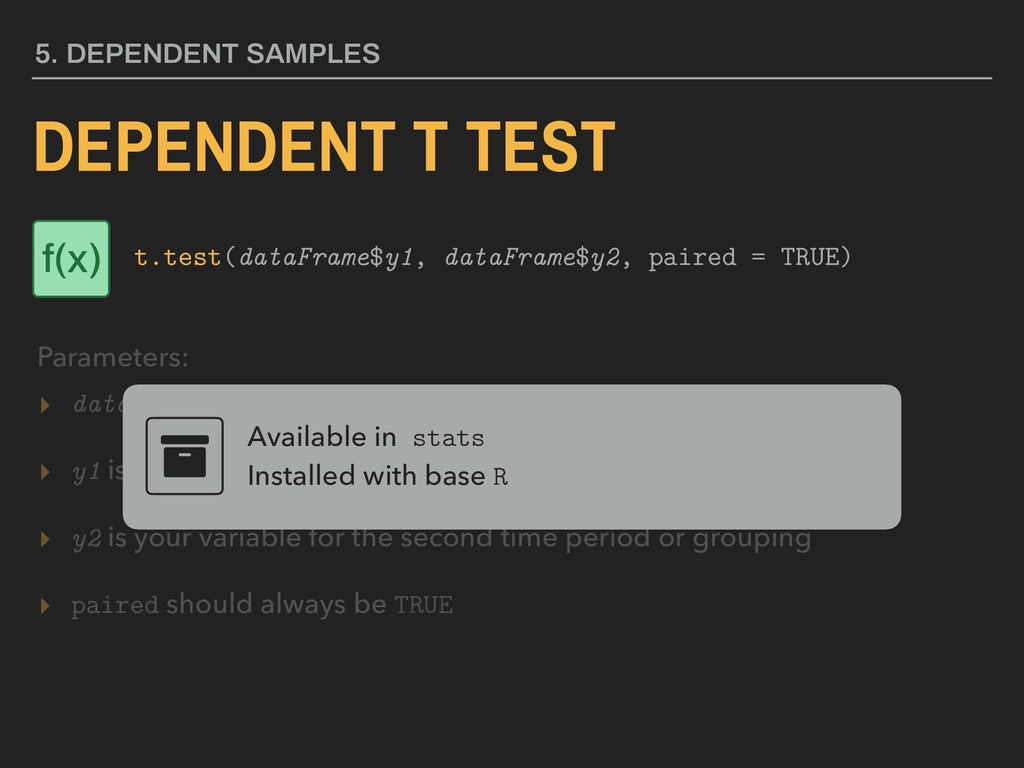
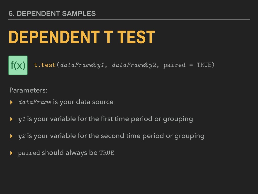
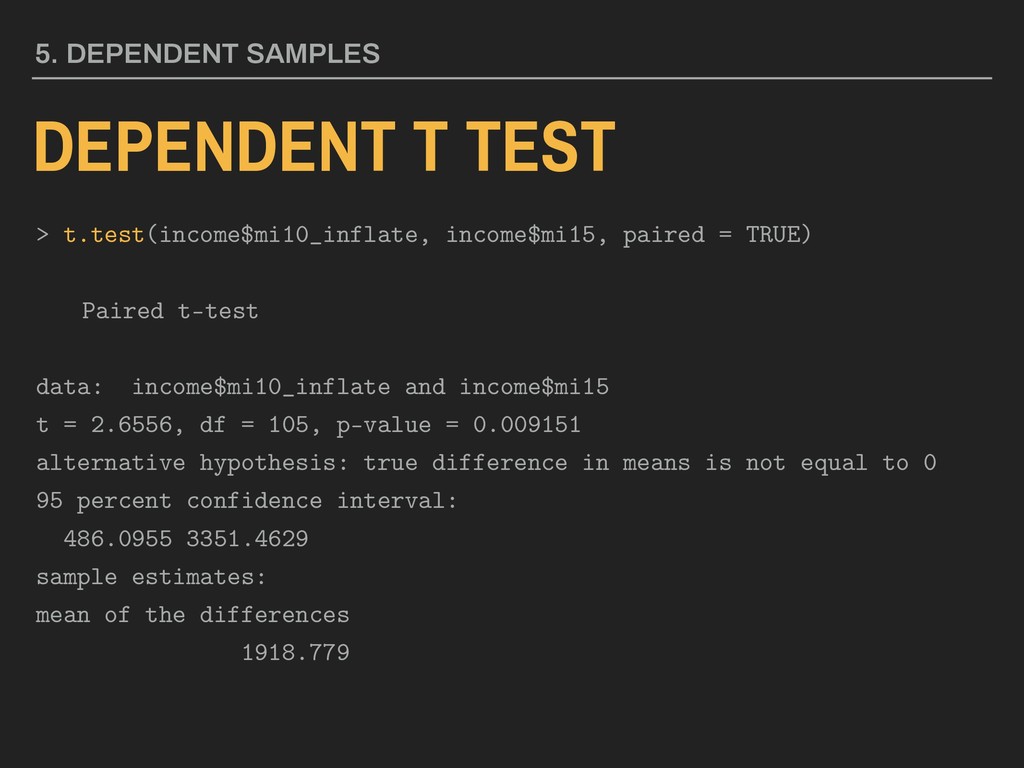
86. ▸ dataFrame is your data source ▸ y1 is your variable for the first time period or grouping ▸ y2 is your variable for the second time period or grouping ▸ paired should always be TRUE Available in stats
 Installed with base R 5. DEPENDENT SAMPLES DEPENDENT T TEST Parameters: t.test(dataFrame$y1, dataFrame$y2, paired = TRUE) f(x)
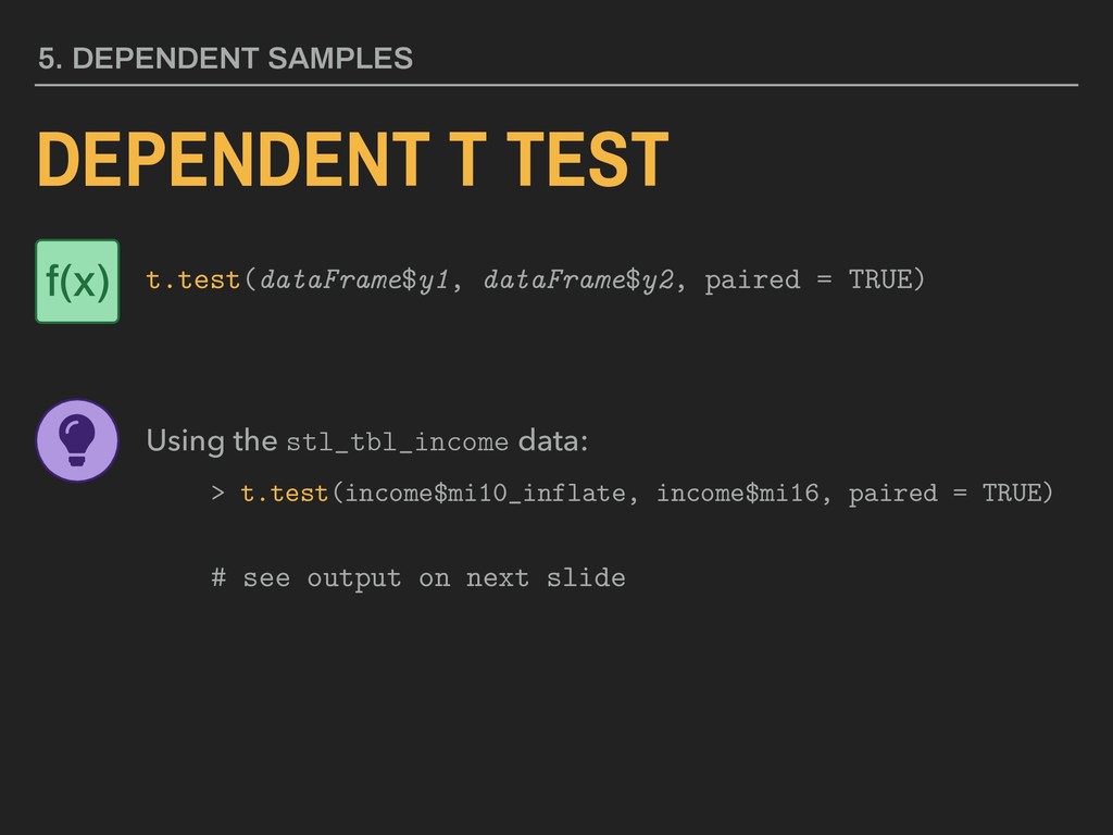
87. ▸ dataFrame is your data source ▸ y1 is your variable for the first time period or grouping ▸ y2 is your variable for the second time period or grouping ▸ paired should always be TRUE 5. DEPENDENT SAMPLES DEPENDENT T TEST Parameters: t.test(dataFrame$y1, dataFrame$y2, paired = TRUE) f(x)
88. DEPENDENT T TEST 5. DEPENDENT SAMPLES t.test(dataFrame$y1, dataFrame$y2, paired = TRUE) Using the stl_tbl_income data: > t.test(income$mi10_inflate, income$mi16, paired = TRUE) # see output on next slide f(x)
89. DEPENDENT T TEST > t.test(income$mi10_inflate, income$mi15, paired = TRUE) Paired t-test data: income$mi10_inflate and income$mi15 t = 2.6556, df = 105, p-value = 0.009151 alternative hypothesis: true difference in means is not equal to 0 95 percent confidence interval: 486.0955 3351.4629 sample estimates: mean of the differences 1918.779 5. DEPENDENT SAMPLES
90. 5. DEPENDENT SAMPLES DEPENDENT T TEST 
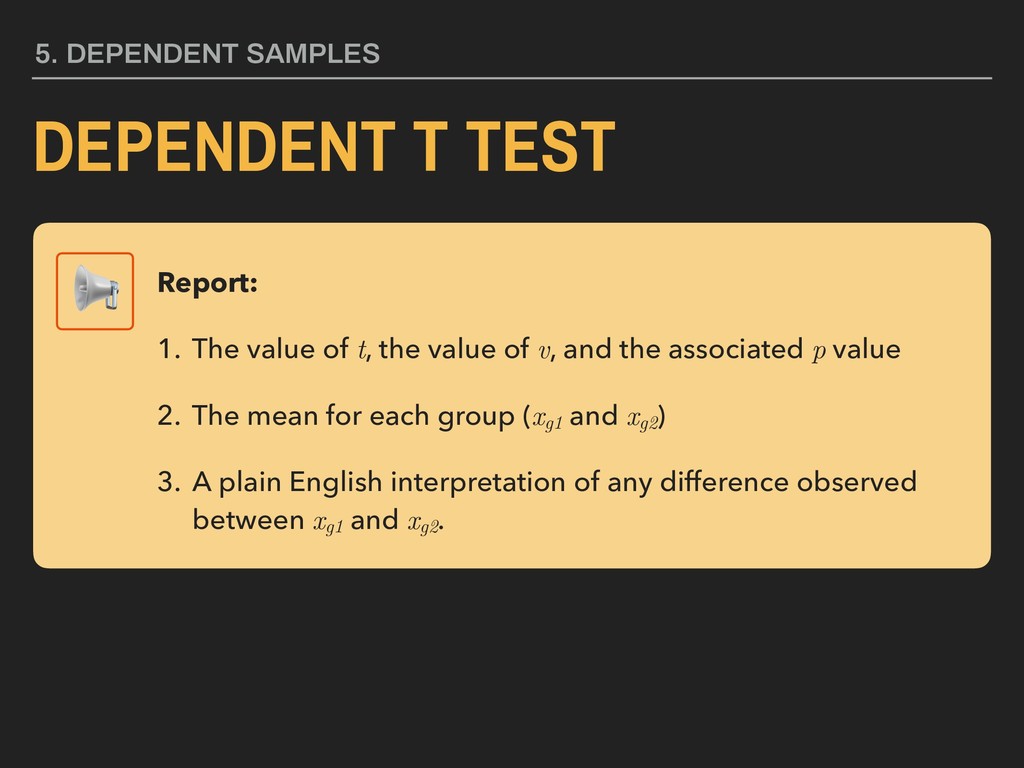
 Report: 1. The value of t, the value of v, and the associated p value 2. The mean for each group (xg1 and xg2 ) 3. A plain English interpretation of any difference observed between xg1 and xg2 .
91. EFFECT SIZES 6
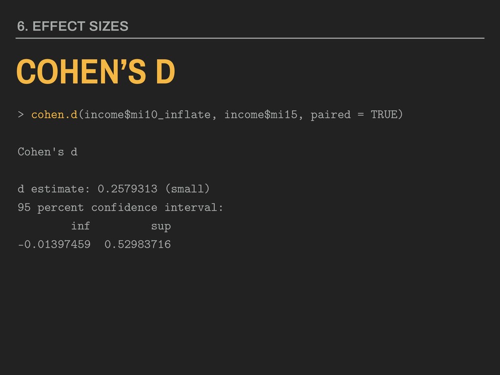
92. ? QUICK REVIEW ▸ An effect size shows use the “real world” significance as opposed to the statistical significance - is the final a “small”, “medium”, or “large” effect? 6. EFFECT SIZES What is an effect size?
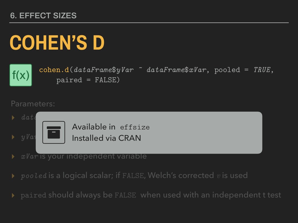
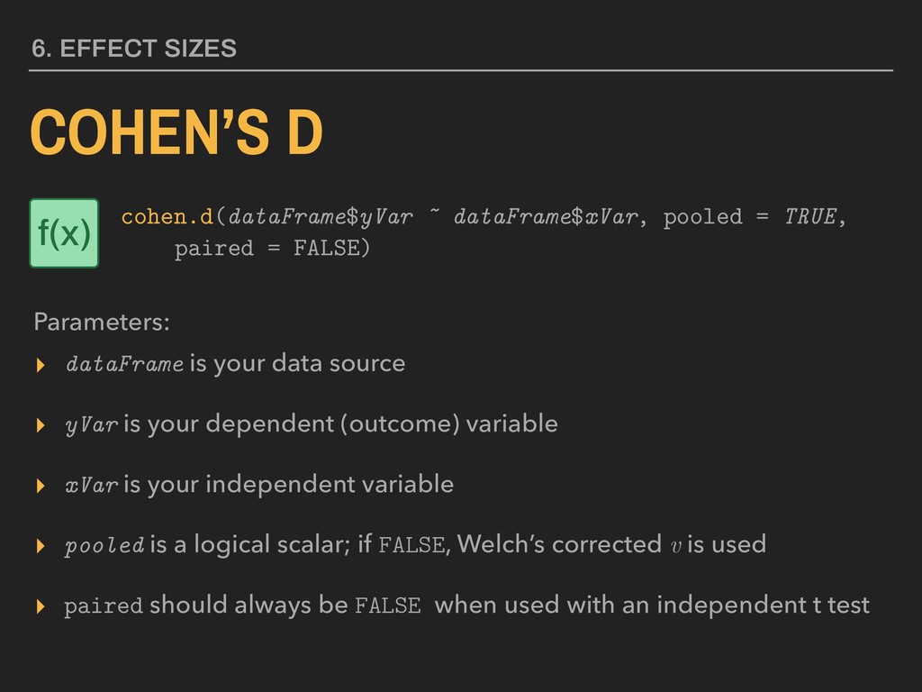
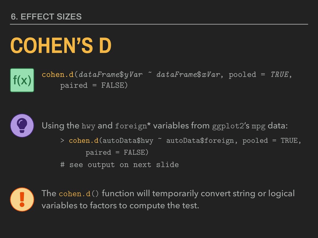
93. ▸ dataFrame is your data source ▸ yVar is your dependent (outcome) variable ▸ xVar is your independent variable ▸ pooled is a logical scalar; if FALSE, Welch’s corrected v is used ▸ paired should always be FALSE when used with an independent t test Available in effsize
 Installed via CRAN 6. EFFECT SIZES COHEN’S D Parameters: cohen.d(dataFrame$yVar ~ dataFrame$xVar, pooled = TRUE, paired = FALSE) f(x)
94. ▸ dataFrame is your data source ▸ yVar is your dependent (outcome) variable ▸ xVar is your independent variable ▸ pooled is a logical scalar; if FALSE, Welch’s corrected v is used ▸ paired should always be FALSE when used with an independent t test 6. EFFECT SIZES COHEN’S D Parameters: cohen.d(dataFrame$yVar ~ dataFrame$xVar, pooled = TRUE, paired = FALSE) f(x)
95. COHEN’S D 6. EFFECT SIZES cohen.d(dataFrame$yVar ~ dataFrame$xVar, pooled = TRUE, paired = FALSE) Using the hwy and foreign* variables from ggplot2’s mpg data: > cohen.d(autoData$hwy ~ autoData$foreign, pooled = TRUE, paired = FALSE) # see output on next slide The cohen.d() function will temporarily convert string or logical variables to factors to compute the test. f(x)
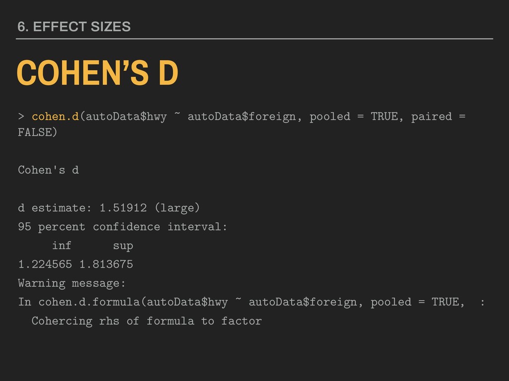
96. COHEN’S D > cohen.d(autoData$hwy ~ autoData$foreign, pooled = TRUE, paired = FALSE) Cohen's d d estimate: 1.51912 (large) 95 percent confidence interval: inf sup 1.224565 1.813675 Warning message: In cohen.d.formula(autoData$hwy ~ autoData$foreign, pooled = TRUE, : Cohercing rhs of formula to factor 6. EFFECT SIZES
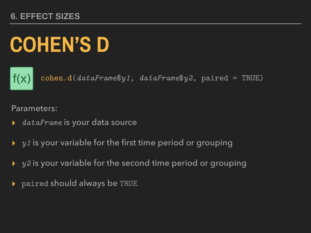
97. ▸ dataFrame is your data source ▸ y1 is your variable for the first time period or grouping ▸ y2 is your variable for the second time period or grouping ▸ paired should always be TRUE 6. EFFECT SIZES COHEN’S D Parameters: cohen.d(dataFrame$y1, dataFrame$y2, paired = TRUE) f(x)
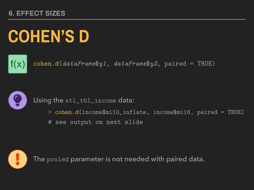
98. COHEN’S D 6. EFFECT SIZES cohen.d(dataFrame$y1, dataFrame$y2, paired = TRUE) Using the stl_tbl_income data: > cohen.d(income$mi10_inflate, income$mi16, paired = TRUE) # see output on next slide f(x) The pooled parameter is not needed with paired data.
99. COHEN’S D > cohen.d(income$mi10_inflate, income$mi15, paired = TRUE) Cohen's d d estimate: 0.2579313 (small) 95 percent confidence interval: inf sup -0.01397459 0.52983716 6. EFFECT SIZES
100. POWER ANALYSES 7
101. 7. POWER ANALYSES REVIEW: STATISTICAL POWER Sample Population µ = µ0 µ ≠ µ0 Not Reject yes Type II Reject Type I yes *The null hypothesis is that µ=µ0 p(Type I)= p(Type II) = β 1-β = power
102. KEY TERM A power analysis is used
 to determine the minimum
 number of observations needed to identify the desired effect.
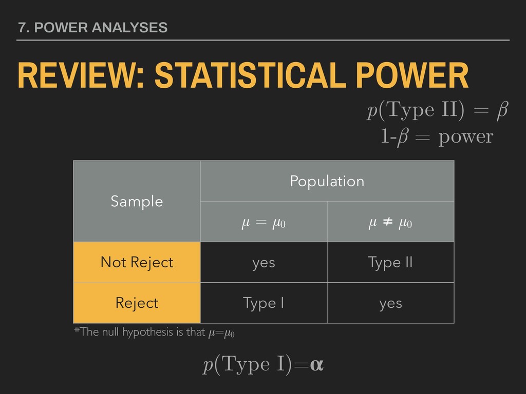
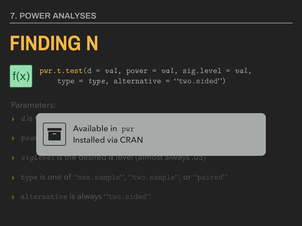
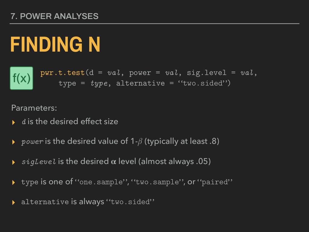
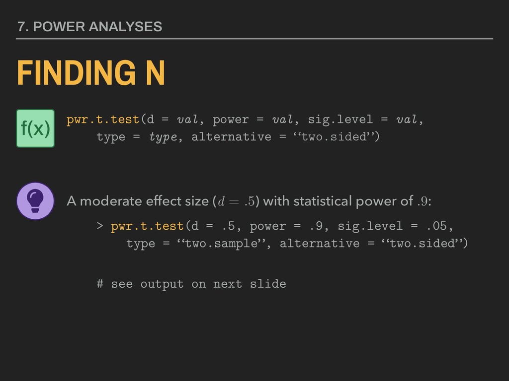
103. ▸ d is the desired effect size ▸ power is the desired value of 1-β (typically at least .8) ▸ sigLevel is the desired level (almost always .05) ▸ type is one of “one.sample”, “two.sample”, or “paired” ▸ alternative is always “two.sided” Available in pwr
 Installed via CRAN 7. POWER ANALYSES FINDING N Parameters: pwr.t.test(d = val, power = val, sig.level = val, 
 type = type, alternative = “two.sided”) f(x)
104. ▸ d is the desired effect size ▸ power is the desired value of 1-β (typically at least .8) ▸ sigLevel is the desired level (almost always .05) ▸ type is one of “one.sample”, “two.sample”, or “paired” ▸ alternative is always “two.sided” 7. POWER ANALYSES FINDING N Parameters: pwr.t.test(d = val, power = val, sig.level = val, 
 type = type, alternative = “two.sided”) f(x)
105. FINDING N 7. POWER ANALYSES pwr.t.test(d = val, power = val, sig.level = val, 
 type = type, alternative = “two.sided”) A moderate effect size (d = .5) with statistical power of .9: > pwr.t.test(d = .5, power = .9, sig.level = .05, type = “two.sample”, alternative = “two.sided”) # see output on next slide f(x)
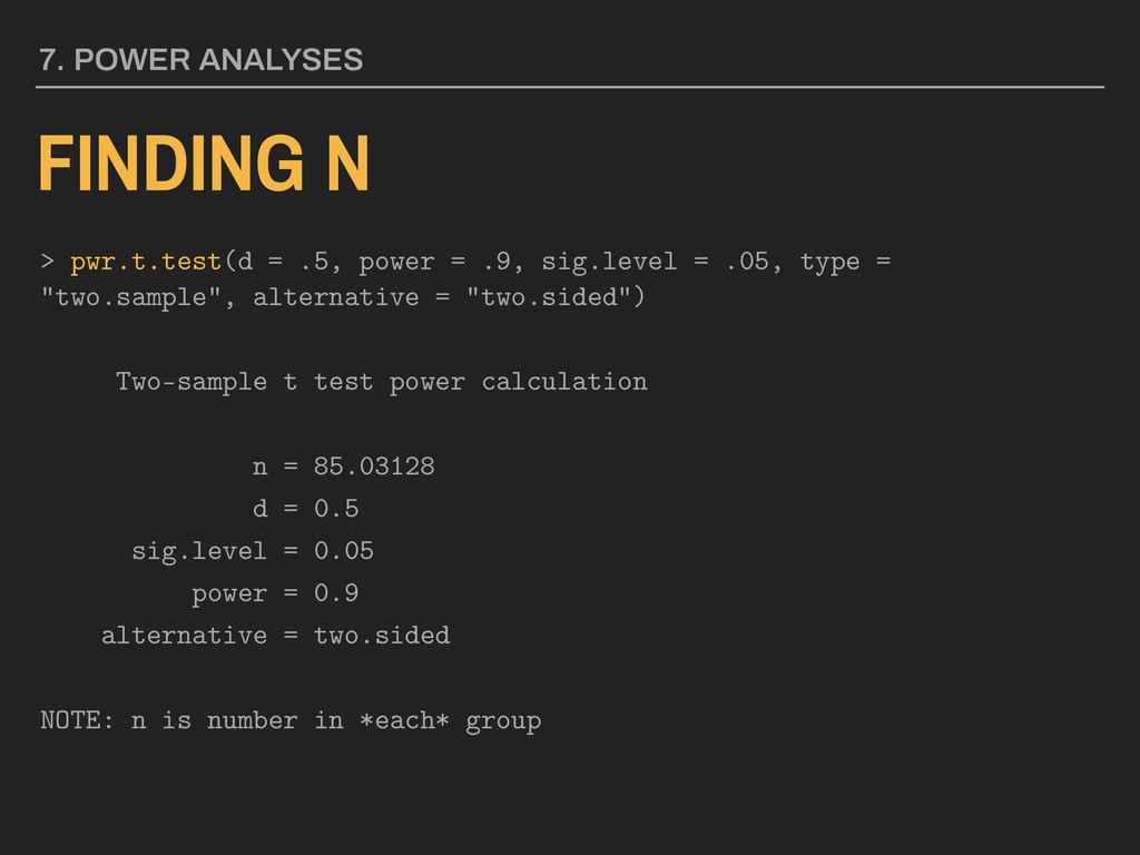
106. FINDING N > pwr.t.test(d = .5, power = .9, sig.level = .05, type = "two.sample", alternative = "two.sided") Two-sample t test power calculation n = 85.03128 d = 0.5 sig.level = 0.05 power = 0.9 alternative = two.sided NOTE: n is number in *each* group 7. POWER ANALYSES
107. 8 BACK 
 MATTER
108. AGENDA REVIEW 7. BACK MATTER 2. Plots for Mean Difference 3. Variance Testing 4. One or Two Samples 5. Dependent Samples 6. Effect Sizes 7. Power Analyses
109. We do not have class next week - a short video lecture will be posted about working with factors and strings. REMINDERS 7. BACK MATTER Lab 08 (from next week) and Lecture Prep 09 (for lecture 10) are due before lecture 10. Lab 07 and Problem Set 04 (from today) are due before 
 lecture 10.