Everything you always wanted to know about text scaling (but were afraid to ask)

Presentation at SFB Workshop on New Methodological Development in Party Manifesto Research, SFB 884, University of Mannheim, October 2012

Transcript

1. Everything you always wanted to know about text scaling˜ (*but were afraid to ask) Will Lowe MZES/SFB/Eurodata, University of Mannheim
2. SFB Workshop, October 2012
3. Disciplinary history Within political science “Category differences” (Laver and Garry, 2000) “MRG compatible coding” (Pennings and Keman, 2002) Wordscores (Laver et al. 2003) R***** I*** P**** (Monroe and Maeda, 2004-ish) Wordfish (Proksch and Slapin, 2007) Different histories in ecology, archaeology, psychology, sociology, applied linguistics, etc. SFB Workshop, October 2012
4. How to take a position Theoretical claims: A position is taken with text using relative proportional emphasis A dimension is a latent variable constructed from counts SFB Workshop, October 2012
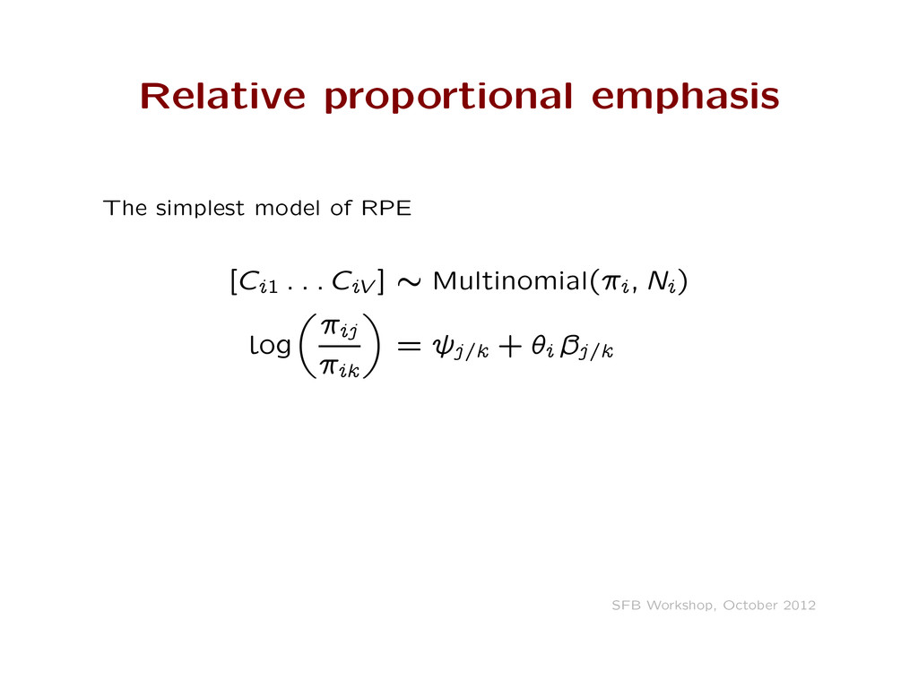
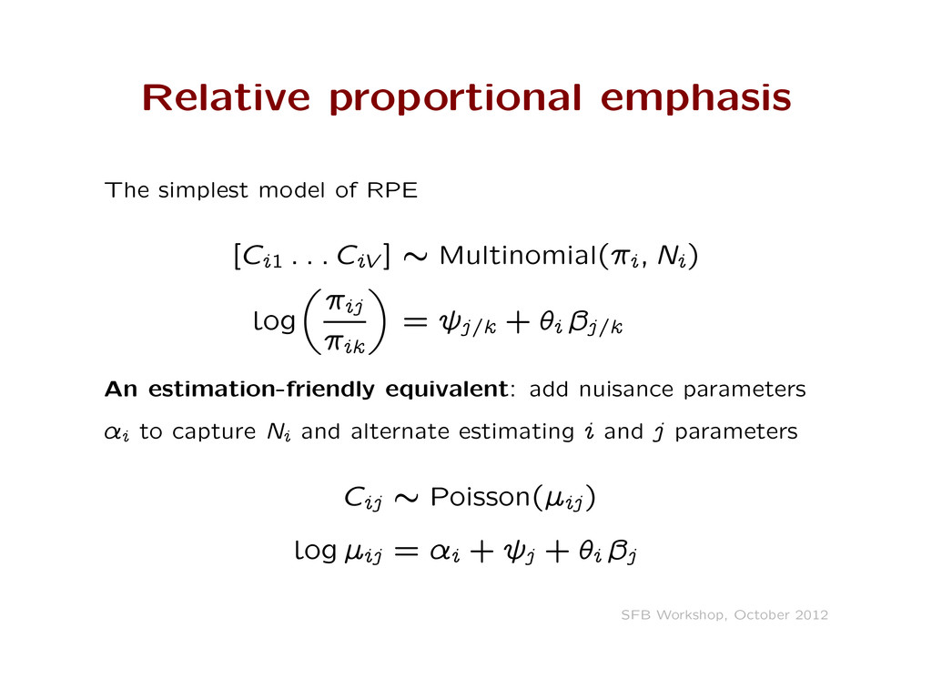
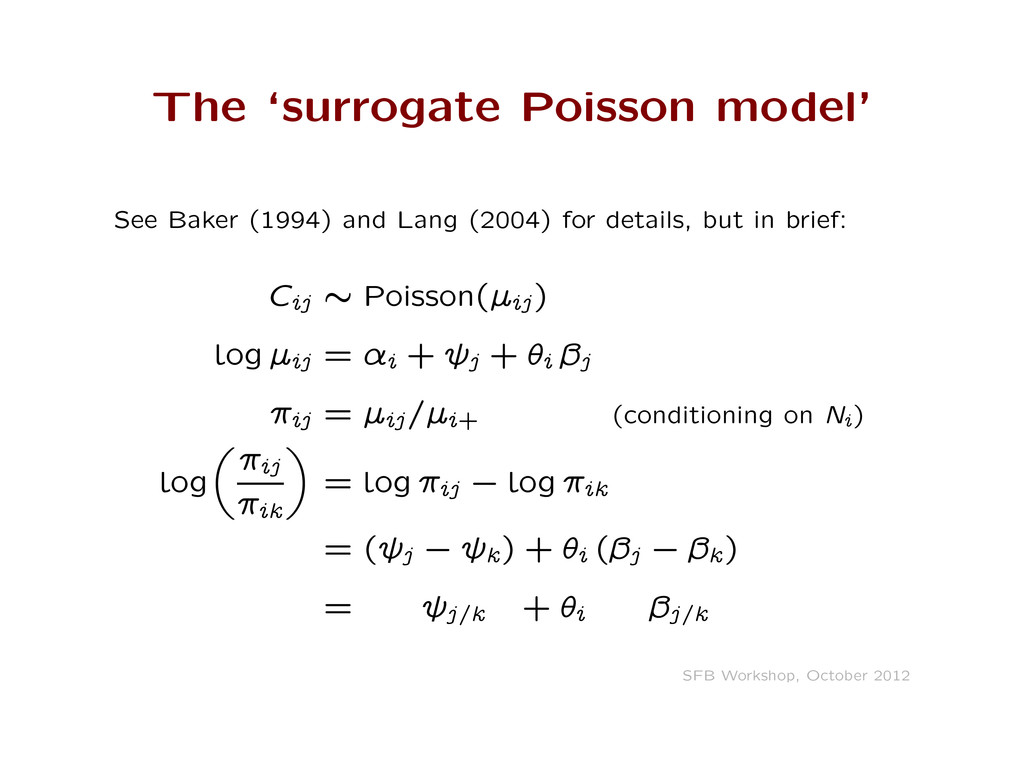
5. How to take a position Theoretical claims: A position is taken with text using relative proportional emphasis A dimension is a latent variable constructed from counts Methodological claims: models of position have a relative proportional emphasis interpretation, usually via logits, wrapped around an embedded low rank approximation SFB Workshop, October 2012
6. How to take a position Theoretical claims: A position is taken with text using relative proportional emphasis A dimension is a latent variable constructed from counts Methodological claims: models of position have a relative proportional emphasis interpretation, usually via logits, wrapped around an embedded low rank approximation There’s only one way to do it SFB Workshop, October 2012
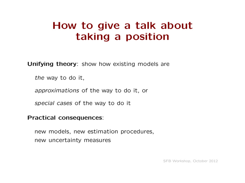
7. How to give a talk about taking a position Unifying theory: show how existing models are the way to do it, approximations of the way to do it, or special cases of the way to do it SFB Workshop, October 2012
8. How to give a talk about taking a position Unifying theory: show how existing models are the way to do it, approximations of the way to do it, or special cases of the way to do it Practical consequences: new models, new estimation procedures, new uncertainty measures SFB Workshop, October 2012
9. Relative proportional emphasis The simplest model of RPE [Ci1 : : : CiV ] ‰ Multinomial(ıi; Ni) log „ıij ıik « = j=k + „i ˛j=k SFB Workshop, October 2012
10. Relative proportional emphasis The simplest model of RPE [Ci1 : : : CiV ] ‰ Multinomial(ıi; Ni) log „ıij ıik « = j=k + „i ˛j=k A no-model version: assume V =2 ^ „i = log „Ci1 + c Ci2 + c « Lowe et al. (2011) SFB Workshop, October 2012
11. Relative proportional emphasis The simplest model of RPE [Ci1 : : : CiV ] ‰ Multinomial(ıi; Ni) log „ıij ıik « = j=k + „i ˛j=k An estimation-friendly equivalent: add nuisance parameters ¸i to capture Ni and alternate estimating i and j parameters Cij ‰ Poisson(—ij) log —ij = ¸i + j + „i ˛j SFB Workshop, October 2012
12. The ‘surrogate Poisson model’ See Baker (1994) and Lang (2004) for details, but in brief: Cij ‰ Poisson(—ij) log —ij = ¸i + j + „i ˛j ıij = —ij=—i+ (conditioning on Ni) log „ıij ıik « = log ıij ` log ıik = ( j ` k) + „i (˛j ` ˛k) = j=k + „i ˛j=k SFB Workshop, October 2012
13. Practical implications: Uncertainty Cheap standard errors: Estimate as Poisson because it’s tractable Assume word parameters and ˛ are well estimated Re-parameterise as Multinomial Use 2nd derivative of the profile Likelihood to compute each „’s standard error No more deeply coupled ¸s to worry about. . . (This is what Austin does) SFB Workshop, October 2012
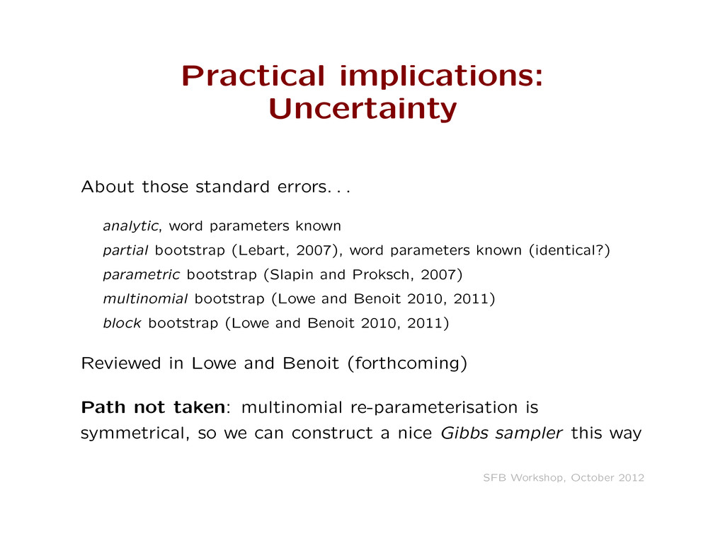
14. Practical implications: Uncertainty About those standard errors. . . analytic, word parameters known partial bootstrap (Lebart, 2007), word parameters known (identical?) parametric bootstrap (Slapin and Proksch, 2007) multinomial bootstrap (Lowe and Benoit 2010, 2011) block bootstrap (Lowe and Benoit 2010, 2011) Reviewed in Lowe and Benoit (forthcoming) SFB Workshop, October 2012
15. Practical implications: Uncertainty About those standard errors. . . analytic, word parameters known partial bootstrap (Lebart, 2007), word parameters known (identical?) parametric bootstrap (Slapin and Proksch, 2007) multinomial bootstrap (Lowe and Benoit 2010, 2011) block bootstrap (Lowe and Benoit 2010, 2011) Reviewed in Lowe and Benoit (forthcoming) Path not taken: multinomial re-parameterisation is symmetrical, so we can construct a nice Gibbs sampler this way SFB Workshop, October 2012
16. Reduced rank approximation A word frequency matrix is a contingency table . . . not a set of survey responses SFB Workshop, October 2012
17. Reduced rank approximation A word frequency matrix is a contingency table . . . not a set of survey responses “Your JedIRT modeling tricks will not work on me” SFB Workshop, October 2012
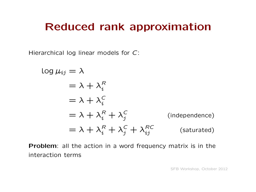
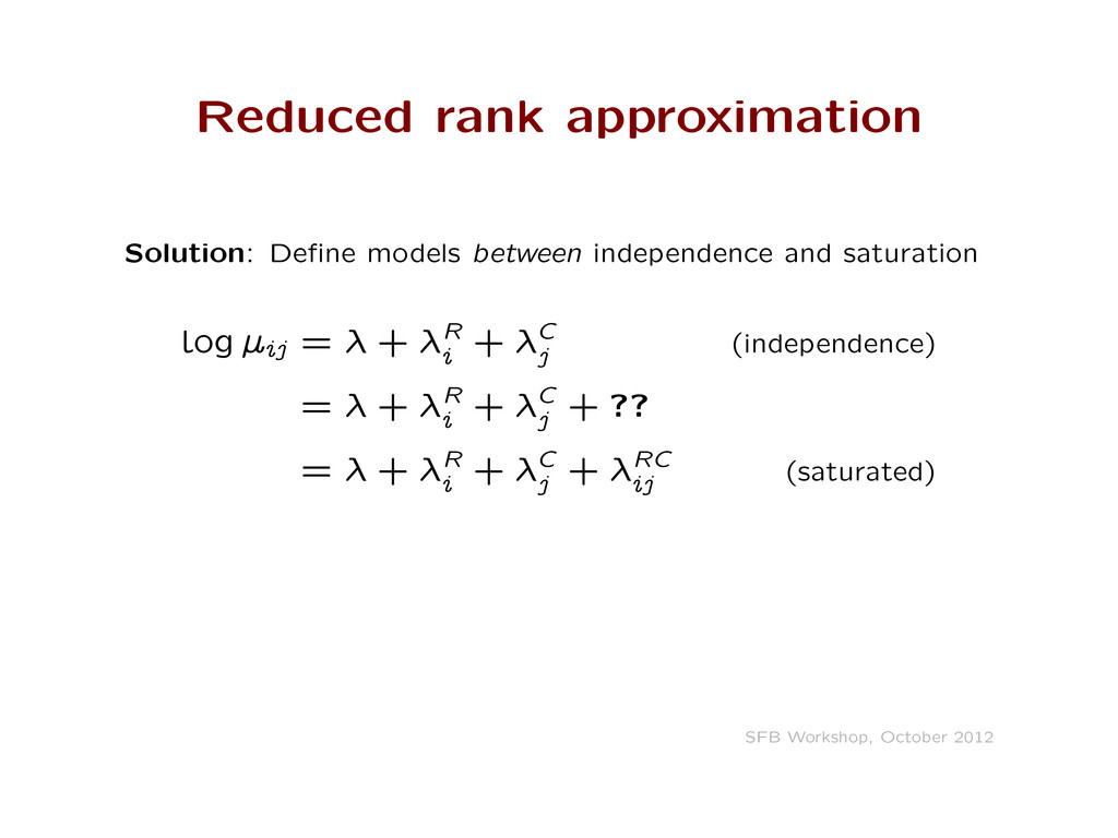
18. Reduced rank approximation Hierarchical log linear models for C: log —ij = – = – + –R i = – + –C i = – + –R i + –C j (independence) = – + –R i + –C j + –RC ij (saturated) Problem: all the action in a word frequency matrix is in the interaction terms SFB Workshop, October 2012
19. Reduced rank approximation Solution: Define models between independence and saturation log —ij = – + –R i + –C j (independence) = – + –R i + –C j + ?? = – + –R i + –C j + –RC ij (saturated) SFB Workshop, October 2012
20. Reduced rank approximation Intuition: –RC = U˚V T (SVD) = M X m u(m)ff(m)vT (m) ı u ff vT (Rank m=1 approx.) SFB Workshop, October 2012
21. Reduced rank approximation Intuition: –RC = U˚V T (SVD) = M X m u(m)ff(m)vT (m) ı u ff vT (Rank m=1 approx.) Now u are document positions (and v are word positions) SFB Workshop, October 2012
22. Implementation Goodman’s Row Column (RC) model embeds the reduced rank approximation in a statistical model log —ij = – + –R i + –C j + ui ff vj SFB Workshop, October 2012
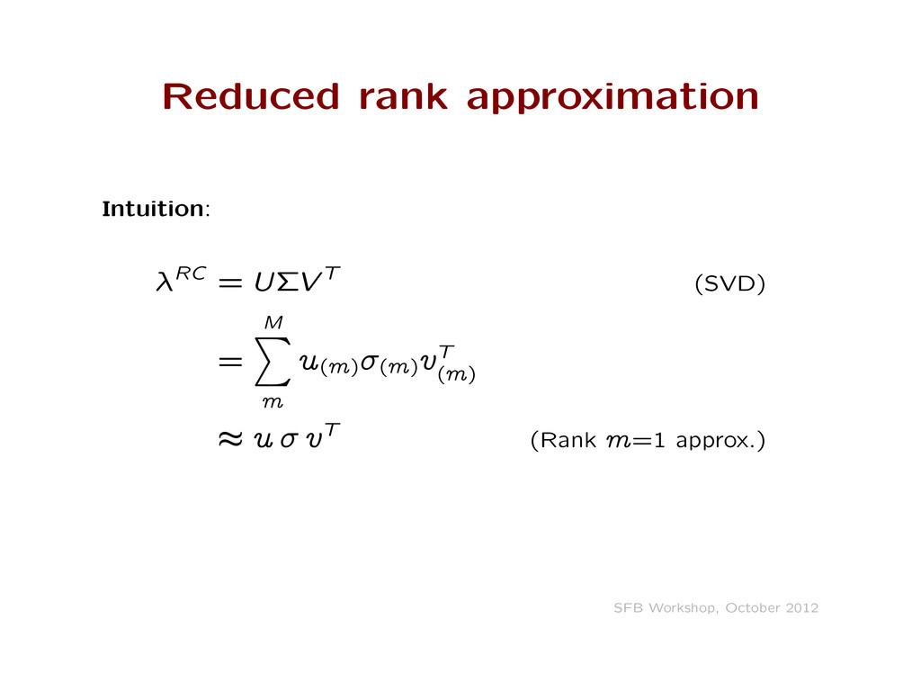
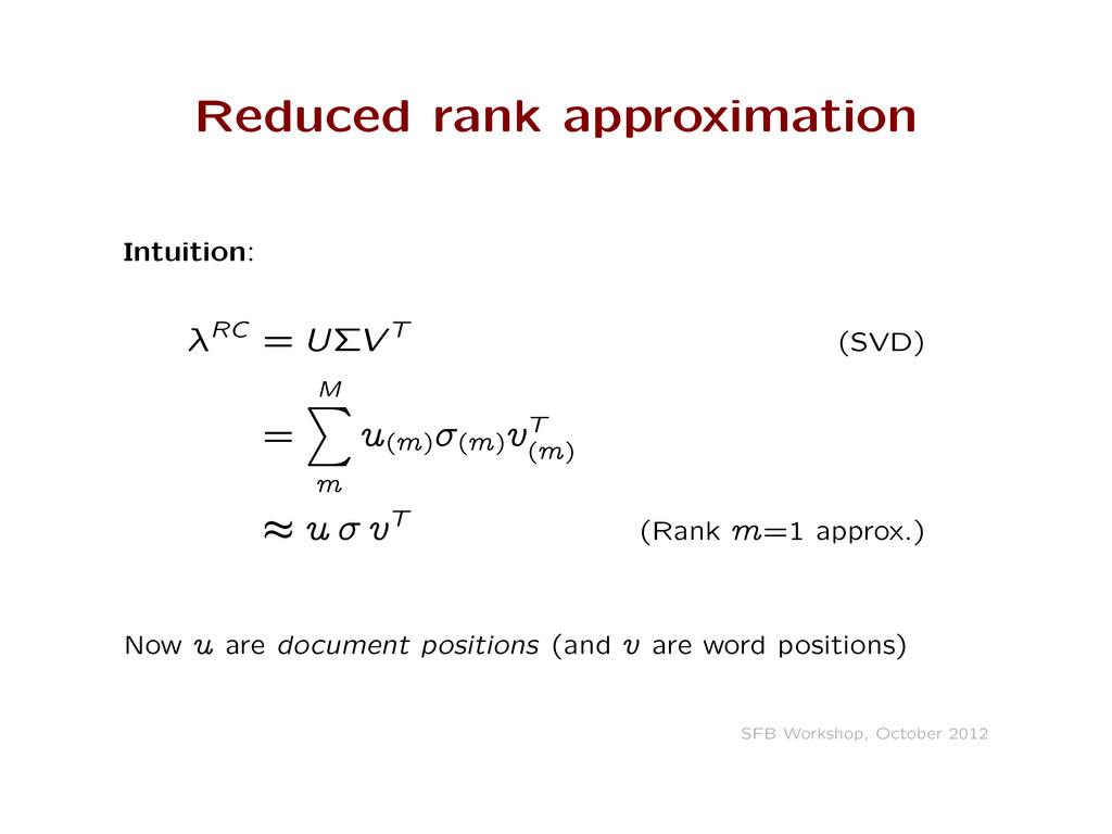
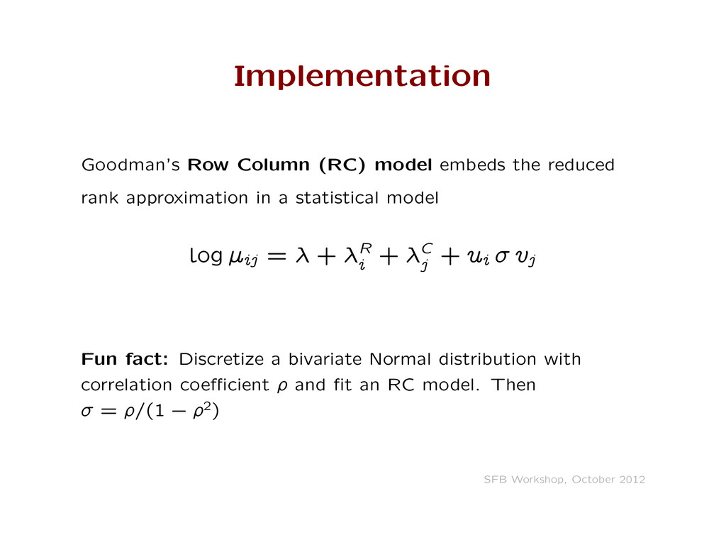
23. Implementation Goodman’s Row Column (RC) model embeds the reduced rank approximation in a statistical model log —ij = – + –R i + –C j + ui ff vj Fun fact: Discretize a bivariate Normal distribution with correlation coefficient  and fit an RC model. Then ff = =(1 ` 2) SFB Workshop, October 2012
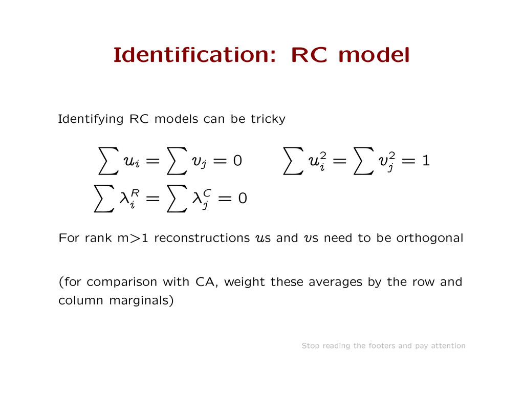
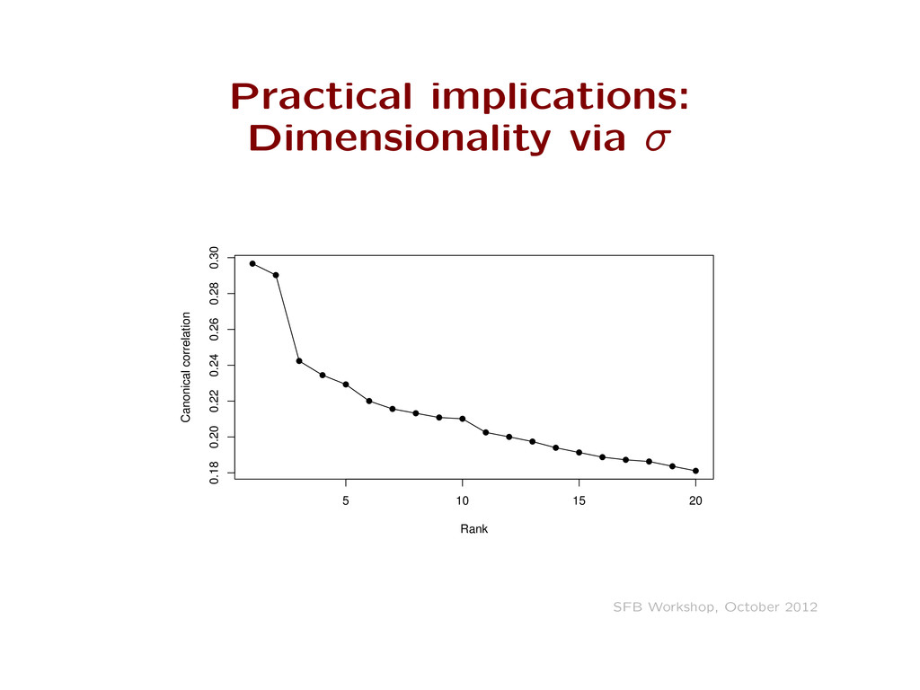
24. Identification: RC model Identifying RC models can be tricky X ui = X vj = 0 X u2 i = X v2 j = 1 X –R i = X –C j = 0 For rank m>1 reconstructions us and vs need to be orthogonal (for comparison with CA, weight these averages by the row and column marginals) Stop reading the footers and pay attention
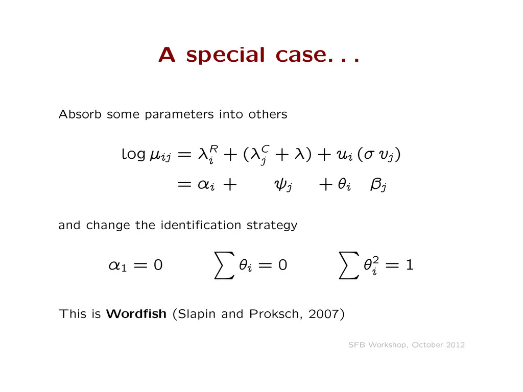
25. A special case. . . Absorb some parameters into others log —ij = –R i + (–C j + –) + ui (ff vj) = ¸i + j + „i ˛j and change the identification strategy ¸1 = 0 X „i = 0 X „2 i = 1 This is Wordfish (Slapin and Proksch, 2007) SFB Workshop, October 2012
26. Identification: Wordfish Changes in ˛’s average can always be offset by changes to ¸ SFB Workshop, October 2012
27. Identification: Wordfish Changes in ˛’s average can always be offset by changes to ¸ Wordfish is not (Likelihood) identified SFB Workshop, October 2012
28. Identification: Wordfish Changes in ˛’s average can always be offset by changes to ¸ Wordfish is not (Likelihood) identified Fortunately a ridge prior on ˛ is sufficient for ‘posterior’ identification (Not really a “technical issue”, as suggested in S&P 2007. . . ) SFB Workshop, October 2012
29. Translation manual Let m and s be the average and standard deviation of ˛ Wordfish to RC RC to Wordfish u ` „ „ ` u v ` (˛ ` m)=s ˛ ` vff + m ff ` s r ` ¸ + „m a ` – + –R ` „m –R ` r ` — r ¸ ` a ` a1 –C ` –C ` — –C ` –C + a1 – ` — r + — –C SFB Workshop, October 2012
30. Practical implications: Statistical properties We get a worked out statistical theory (Goodman, Haberman, Gilula, Becker) for free from the RC model literature, e.g. diagnostics, including for extra dimensions model extensions, e.g. parameterised „, K-way tables two more estimation algorithms SFB Workshop, October 2012
31. Practical implications: Dimensionality via ff q q q q q q q q q q q q q q q q q q q q 5 10 15 20 0.18 0.20 0.22 0.24 0.26 0.28 0.30 Rank Canonical correlation SFB Workshop, October 2012
32. Least squares approximation Correspondence analysis constructs a reduced rank approximation directly from counts SFB Workshop, October 2012
33. Least squares approximation Correspondence analysis constructs a reduced rank approximation directly from counts Construct word probabilities P from C (divide by total). SFB Workshop, October 2012
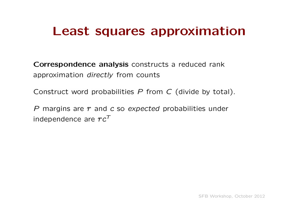
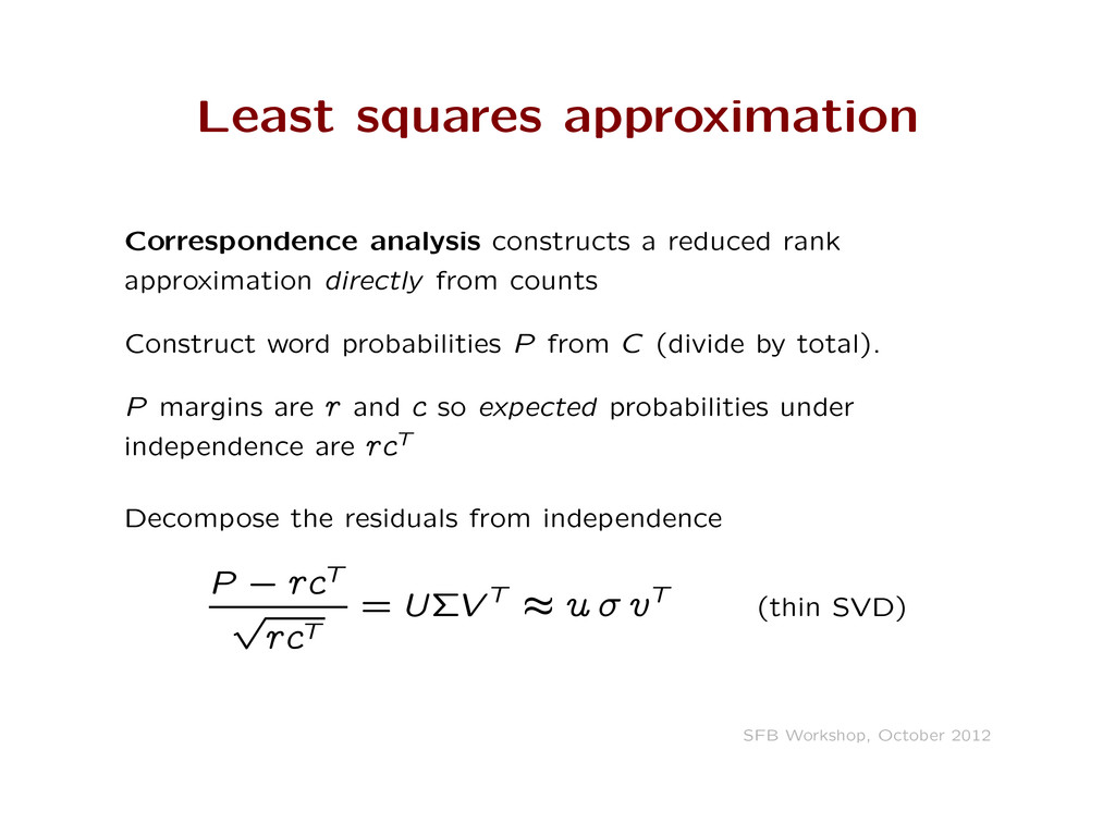
34. Least squares approximation Correspondence analysis constructs a reduced rank approximation directly from counts Construct word probabilities P from C (divide by total). P margins are r and c so expected probabilities under independence are rcT SFB Workshop, October 2012
35. Least squares approximation Correspondence analysis constructs a reduced rank approximation directly from counts Construct word probabilities P from C (divide by total). P margins are r and c so expected probabilities under independence are rcT Decompose the residuals from independence P ` rcT p rcT = U˚V T ı u ff vT (thin SVD) SFB Workshop, October 2012
36. Least squares approximation This implies the low rank reconstruction Pij ı ri cj (1 + ui ff vj) SFB Workshop, October 2012
37. Least squares approximation This implies the low rank reconstruction Pij ı ri cj (1 + ui ff vj) This is also a type of unfolding model for count data (ter Braak, 1981) SFB Workshop, October 2012
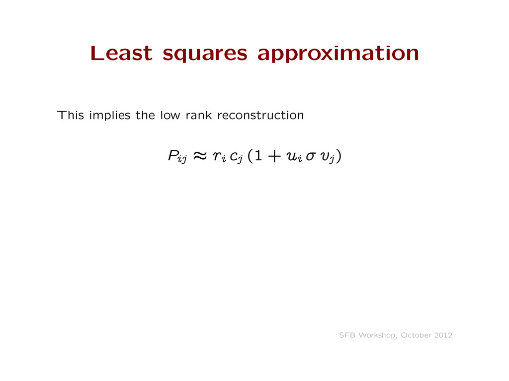
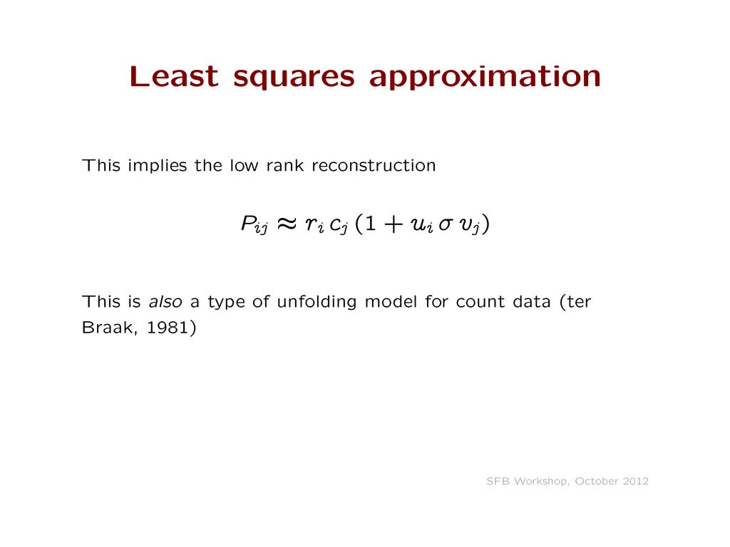
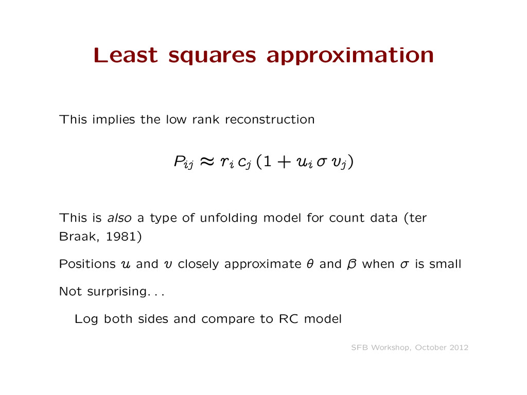
38. Least squares approximation This implies the low rank reconstruction Pij ı ri cj (1 + ui ff vj) This is also a type of unfolding model for count data (ter Braak, 1981) Positions u and v closely approximate „ and ˛ when ff is small Not surprising. . . Log both sides and compare to RC model SFB Workshop, October 2012
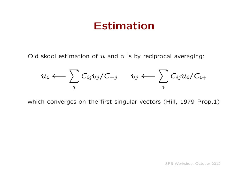
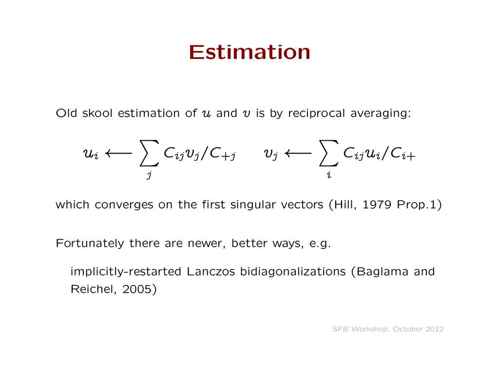
39. Estimation Old skool estimation of u and v is by reciprocal averaging: ui ` X j Cijvj=C+j vj ` X i Cijui=Ci+ which converges on the first singular vectors (Hill, 1979 Prop.1) SFB Workshop, October 2012
40. Estimation Old skool estimation of u and v is by reciprocal averaging: ui ` X j Cijvj=C+j vj ` X i Cijui=Ci+ which converges on the first singular vectors (Hill, 1979 Prop.1) Fortunately there are newer, better ways, e.g. implicitly-restarted Lanczos bidiagonalizations (Baglama and Reichel, 2005) SFB Workshop, October 2012
41. A special case. . . If we decide that we know scores u for ‘reference’ documents treat document with unknown scores as out-of-sample (‘virgin documents’) then we can compute word ‘scores’ v in one step, and new documents scores in one more step. SFB Workshop, October 2012
42. A special case. . . If we decide that we know scores u for ‘reference’ documents treat document with unknown scores as out-of-sample (‘virgin documents’) then we can compute word ‘scores’ v in one step, and new documents scores in one more step. This is Wordscores (Laver et al. 2003; Lowe, 2008) SFB Workshop, October 2012
43. Practical implications We do better by treating unknown document scores as in-sample and estimating their scores SFB Workshop, October 2012
44. Practical implications We do better by treating unknown document scores as in-sample and estimating their scores Beats Wordscores on its own toy non-stochastic example! 5 reference document scores, one unknown true value `0:45 Wordscores `0:448 plus 8 iterations `0:450 Started in the right direction, then stopped. SFB Workshop, October 2012
45. Practical implications We do better by treating unknown document scores as in-sample and estimating their scores Beats Wordscores on its own toy non-stochastic example! 5 reference document scores, one unknown true value `0:45 Wordscores `0:448 plus 8 iterations `0:450 Started in the right direction, then stopped. This will also work for Wordfish. . . SFB Workshop, October 2012
46. Practical implications This will also work for Wordfish. . . Fix positions on > 2 ‘reference’ documents Only update positions of other documents Unit normalise as before (yes, this maintains reference scores!) SFB Workshop, October 2012
47. Things we still always wanted to know When does the reference score strategy work well? How do we build models of document position? (for CA this is known) How do we scale up to serious numbers of documents SFB Workshop, October 2012
48. Code R-package Austin: Code / collaboration welcome. . . SFB Workshop, October 2012