Upgrade to Pro — share decks privately, control downloads, hide ads and more …

Ph.D. Qualifying 2016

Ph.D. Qualifying 2016

The presentation for my Ph.D. qualifying of 2016. This is the undergoing projects and plans for my Ph.D.

Marco De Nadai

November 17, 2016
Tweet

More Decks by Marco De Nadai

Other Decks in Research

Transcript

  1. By 2010 urban population began to exceed the rural one

    UN population division, 2010 Urban Rural Population:
  2. By 2010 urban population began to exceed the rural one

    UN population division, 2010 90% of global gross added value comes from urban areas (2006) Urban Rural Population:
  3. Cities, very difficult to explain 4 COMPLEX Not only agglomeration

    of residents, factories, shops • Millions of individuals • Continuously evolving A small change generates a cascading throughout
  4. The role of data mining and machine learning 5 DATA

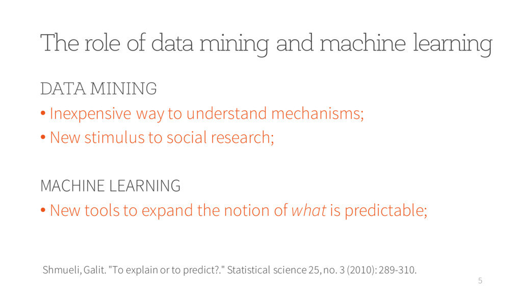
    MINING • Inexpensive way to understand mechanisms; • New stimulus to social research; MACHINE LEARNING • New tools to expand the notion of what is predictable; Shmueli, Galit. "To explain or to predict?." Statistical science 25, no. 3 (2010): 289-310.
  5. Predict deprivation and per-capita income solely relying on mobility diversity

    and social diversity 6 Pappalardo, L., Vanhoof, M., Gabrielli, L., Smoreda, Z., Pedreschi, D., & Giannotti, F. (2016). An analytical framework to nowcast well-being using mobile phone data. International Journal of Data Science and Analytics
  6. Predict poverty from satellite imagery (75% variation of economic outcomes)

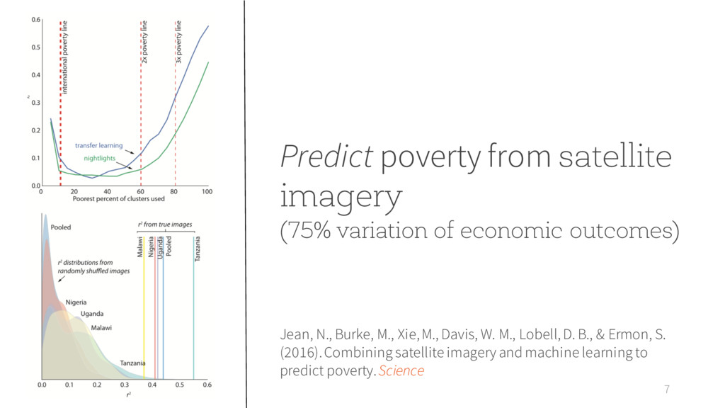
    7 Jean, N., Burke, M., Xie, M., Davis, W. M., Lobell, D. B., & Ermon, S. (2016). Combining satellite imagery and machine learning to predict poverty. Science
  7. Predict crime rates from POIs, mobility, demographics 8 Wang, H.,

    Kifer, D., Graif, C., & Li, Z. (2016). Crime rate inference with big data. In Proceedings of the 22nd ACM SIGKDD.
  8. Understand underlying mechanisms of a city 9 Arbesman, Samuel. Overcomplicated:

    Technology at the Limits of Comprehension. Penguin, 2016. Describe
  9. Understand underlying mechanisms of a city 10 Arbesman, Samuel. Overcomplicated:

    Technology at the Limits of Comprehension. Penguin, 2016. Describe Predict
  10. Understand underlying mechanisms of a city 11 Arbesman, Samuel. Overcomplicated:

    Technology at the Limits of Comprehension. Penguin, 2016. Describe Predict Generate
  11. Understand underlying mechanisms of a city 12 Arbesman, Samuel. Overcomplicated:

    Technology at the Limits of Comprehension. Penguin, 2016. Describe Predict Generate
  12. A multitude of dimensions and aspects! 16 Urban vitality 1

    Security perception 2 DONE ON-GOING / FUTURE
  13. A multitude of dimensions and aspects! 17 Crime 3 Urban

    vitality 1 Security perception 2 DONE ON-GOING / FUTURE
  14. A multitude of dimensions and aspects! 18 Crime 3 Urban

    vitality 1 Security perception 2 Structural design 4 DONE ON-GOING / FUTURE
  15. A multitude of dimensions and aspects! 19 DESCRIBE & PREDICT

    Crime 3 Urban vitality 1 Security perception 2 Structural design 4 DONE ON-GOING / FUTURE
  16. A multitude of dimensions and aspects! 20 DESCRIBE & PREDICT

    PREDICT & GENERATE Crime 3 Urban vitality 1 Security perception 2 Structural design 4 DONE ON-GOING / FUTURE
  17. Urban Vitality OBJECTIVE CHARACTERISTICS Q: Can we describe and predict

    vitality from urban physical characteristics?
  18. The theory: Jane Jacobs One of the most influential books

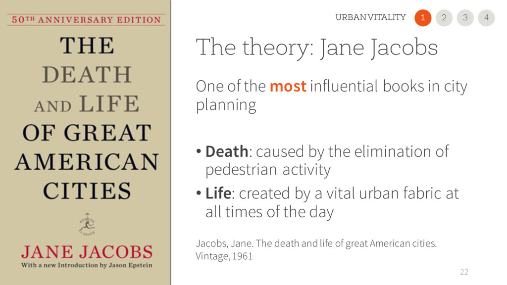
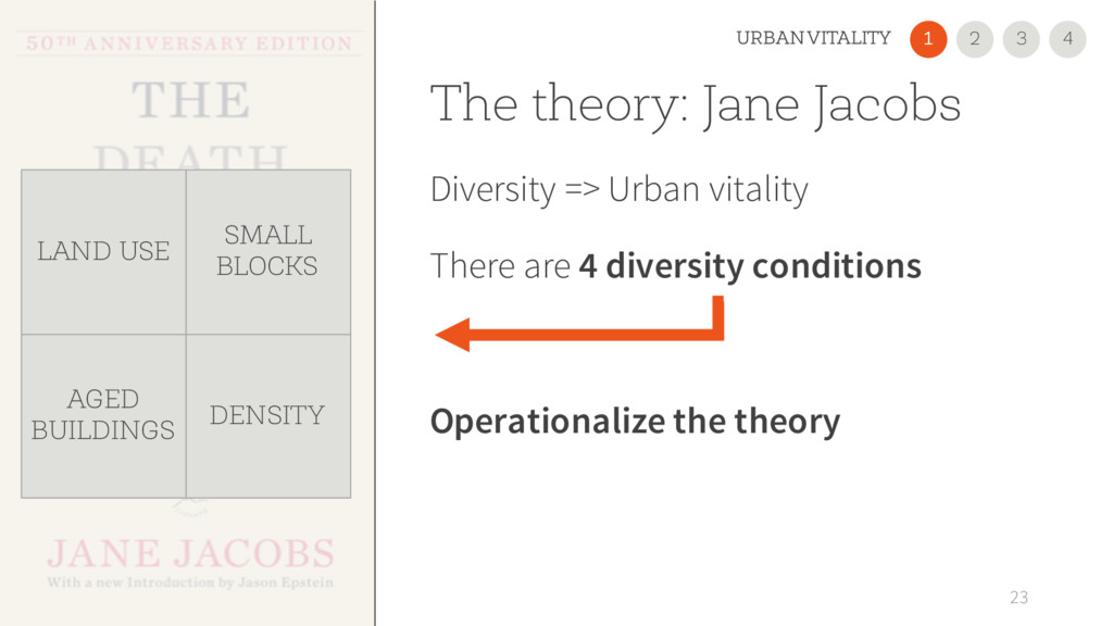
    in city planning • Death: caused by the elimination of pedestrian activity • Life: created by a vital urban fabric at all times of the day 22 Jacobs, Jane. The death and life of great American cities. Vintage, 1961 2 1 3 URBAN VITALITY 4
  19. The theory: Jane Jacobs Diversity => Urban vitality There are

    4 diversity conditions Operationalize the theory 23 LAND USE SMALL BLOCKS AGED BUILDINGS DENSITY 2 1 3 URBAN VITALITY 4
  20. The theory: Jane Jacobs 2+ primary uses (contemporarily) 24 LAND

    USE SMALL BLOCKS AGED BUILDINGS DENSITY 2 1 3 URBAN VITALITY 4
  21. The theory: Jane Jacobs 2+ primary uses (contemporarily) 25 LAND

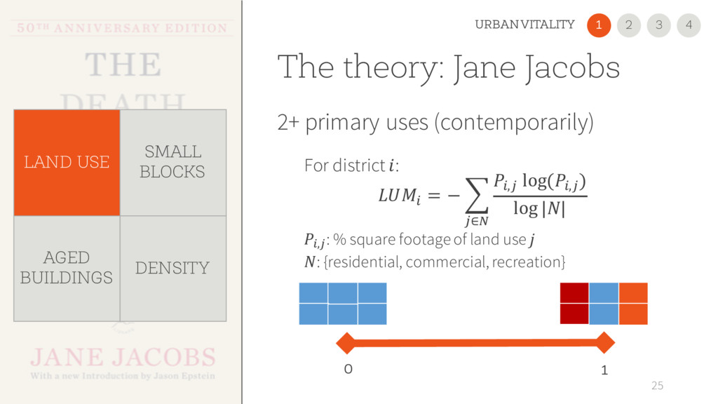
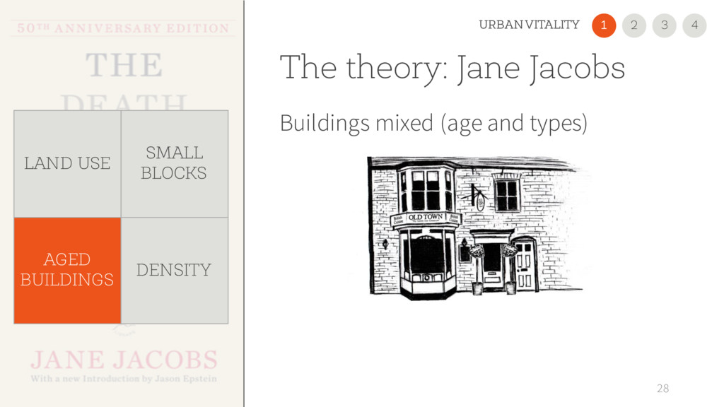
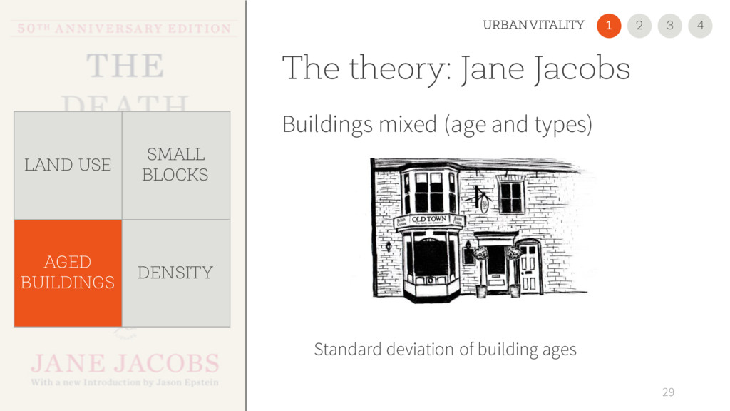
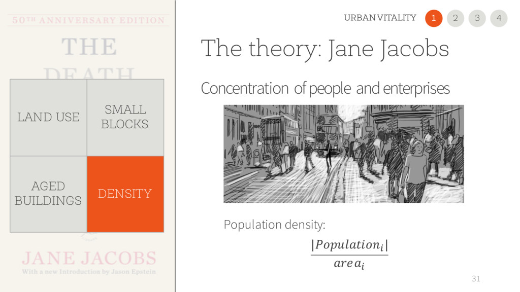
    USE SMALL BLOCKS AGED BUILDINGS DENSITY For district : % = − ( %,+ log (%,+ ) log || +∈5 %,+: % square footage of land use : {residential, commercial, recreation} 1 0 2 1 3 URBAN VITALITY 4
  22. The theory: Jane Jacobs City blocks should be small/short 26

    LAND USE SMALL BLOCKS AGED BUILDINGS DENSITY BLOCKS 2 1 3 URBAN VITALITY 4
  23. The theory: Jane Jacobs City blocks should be small/short 27

    LAND USE SMALL BLOCKS AGED BUILDINGS DENSITY BLOCKS For district : |% | % 2 1 3 URBAN VITALITY 4
  24. The theory: Jane Jacobs Buildings mixed (age and types) 28

    LAND USE SMALL BLOCKS AGED BUILDINGS DENSITY 2 1 3 URBAN VITALITY 4
  25. The theory: Jane Jacobs Buildings mixed (age and types) 29

    LAND USE SMALL BLOCKS AGED BUILDINGS DENSITY Standard deviation of building ages 2 1 3 URBAN VITALITY 4
  26. The theory: Jane Jacobs Concentration of people and enterprises 30

    LAND USE SMALL BLOCKS AGED BUILDINGS DENSITY 2 1 3 URBAN VITALITY 4
  27. The theory: Jane Jacobs Concentration of people and enterprises 31

    LAND USE SMALL BLOCKS AGED BUILDINGS DENSITY Population density: |% | % 2 1 3 URBAN VITALITY 4
  28. Vitality Anonymized Mobile phone Internet activity as a proxy for

    urban vitality 32 1 % || ( | % | G∈H : set of hours (180 days x 24h) : area of district 2 1 3 URBAN VITALITY 4
  29. The Death and Life of Great Italian Cities 33 DATA

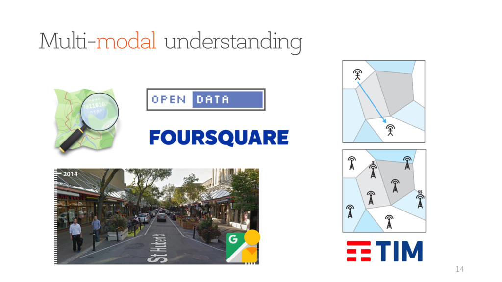
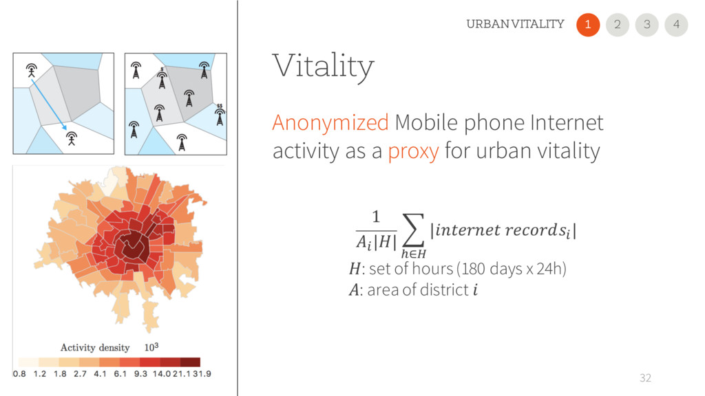
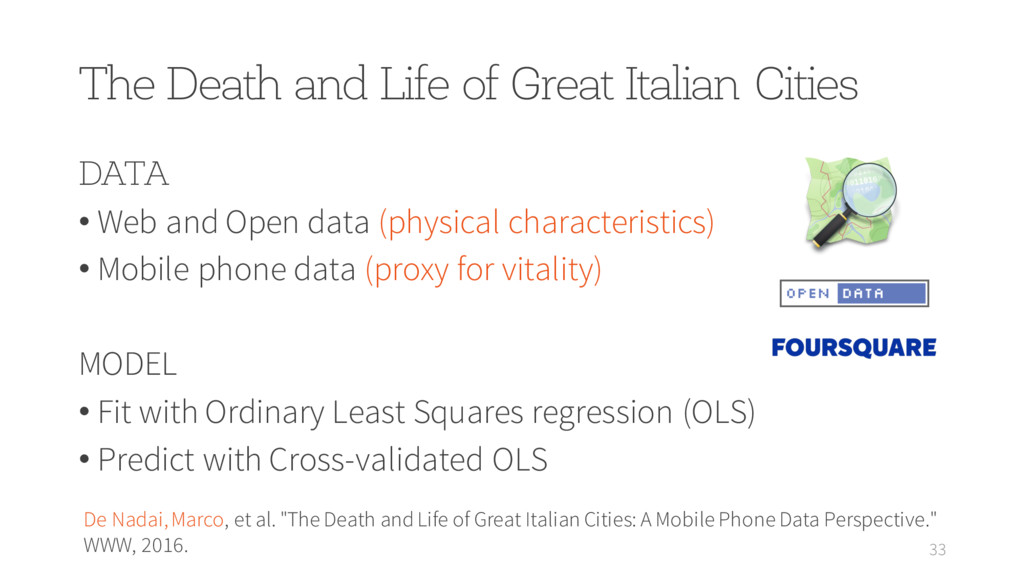
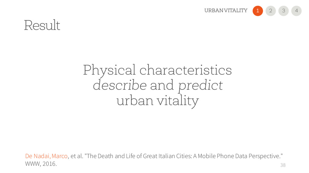
    • Web and Open data (physical characteristics) • Mobile phone data (proxy for vitality) MODEL • Fit with Ordinary Least Squares regression (OLS) • Predict with Cross-validated OLS De Nadai, Marco, et al. "The Death and Life of Great Italian Cities: A Mobile Phone Data Perspective." WWW, 2016.
  30. The log Linear Regression 34 Vitality (Ground truth) = K

    K + N N + ⋯ + P P + 2 1 3 URBAN VITALITY 4
  31. The log Linear Regression 35 Vitality (Ground truth) Land Use

    Mix = K K + N N + ⋯ + P P + 2 1 3 URBAN VITALITY 4
  32. The log Linear Regression 36 Vitality (Ground truth) Land Use

    Mix Employment density = K K + N N + ⋯ + P P + 2 1 3 URBAN VITALITY 4
  33. 37 Urban metric Beta coefficient Employmentdensity 0.434*** Intersections density 0.191***

    Housing types 0.185*** Closeness highways -0.102*** 3rd places x closenesshighways 0.07** Closeness parks x closeness highways -0.07*** adj − RN 0.77 *** p-value < 0.001; ** p-value < 0.01; Describe urban vitality 2 1 3 URBAN VITALITY 4
  34. Result 38 De Nadai, Marco, et al. "The Death and

    Life of Great Italian Cities: A Mobile Phone Data Perspective." WWW, 2016. Physical characteristics describe and predict urban vitality 2 1 3 URBAN VITALITY 4
  35. Security perception SUBJECTIVE CHARACTERISTICS Q: how can new sources of

    data and deep learning models help to link urban visual perception and the behavior of people?
  36. Broken windows theory • City mismanagement • Dirty places •

    Poor infrastructure Lead to misbehavior => Crime 40 Wilson, James Q., and George L. Kelling. "Broken windows." Critical issues in policing: Contemporary readings (1982): 395- 407. 2 1 3 SECURITY PERCEPTION 4
  37. Are Safer Looking Neighborhoods More Lively? 41 DATA • Web

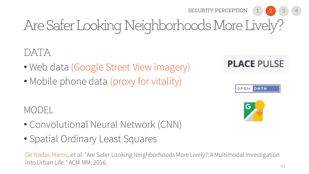
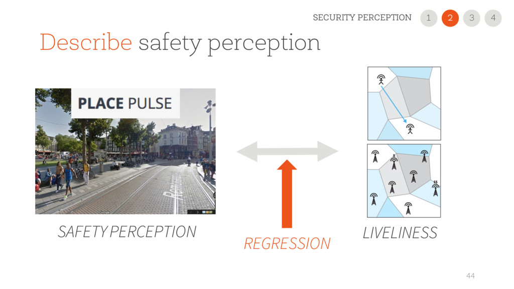
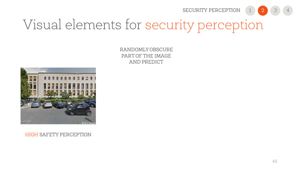
    data (Google Street View imagery) • Mobile phone data (proxy for vitality) MODEL • Convolutional Neural Network (CNN) • Spatial Ordinary Least Squares De Nadai, Marco, et al. "Are Safer Looking Neighborhoods More Lively?: A Multimodal Investigation into Urban Life." ACM MM, 2016. 1 SECURITY PERCEPTION 4 2 3
  38. Place Pulse 2.0 42 1 SECURITY PERCEPTION 4 Salesses, P.,

    Schechtner, K., & Hidalgo, C. A. (2013). The collaborative image of the city: mapping the inequality of urban perception. PloS one 2 3
  39. Security perception prediction • Learning safety perception, predict in Rome

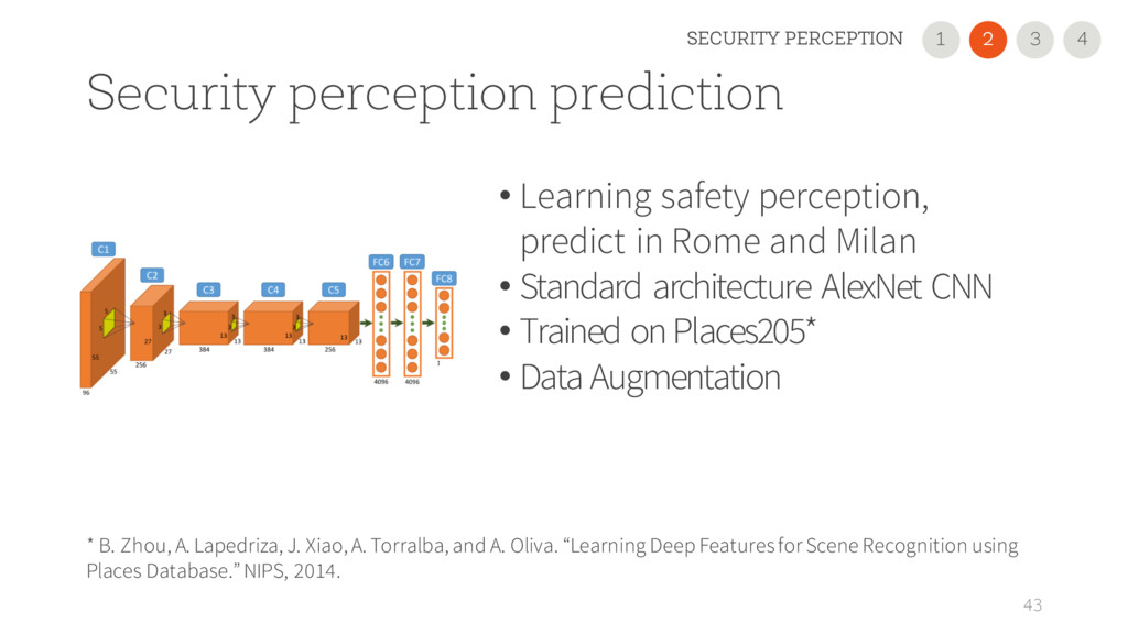
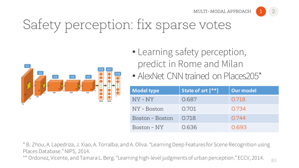
    and Milan • Standard architecture AlexNet CNN • Trained on Places205* • Data Augmentation 43 * B. Zhou, A. Lapedriza, J. Xiao, A. Torralba, and A. Oliva. “Learning Deep Features for Scene Recognition using Places Database.” NIPS, 2014. 1 SECURITY PERCEPTION 4 2 3
  40. Security perception <-> presence of people 45 Urban metric Beta

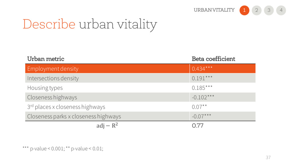
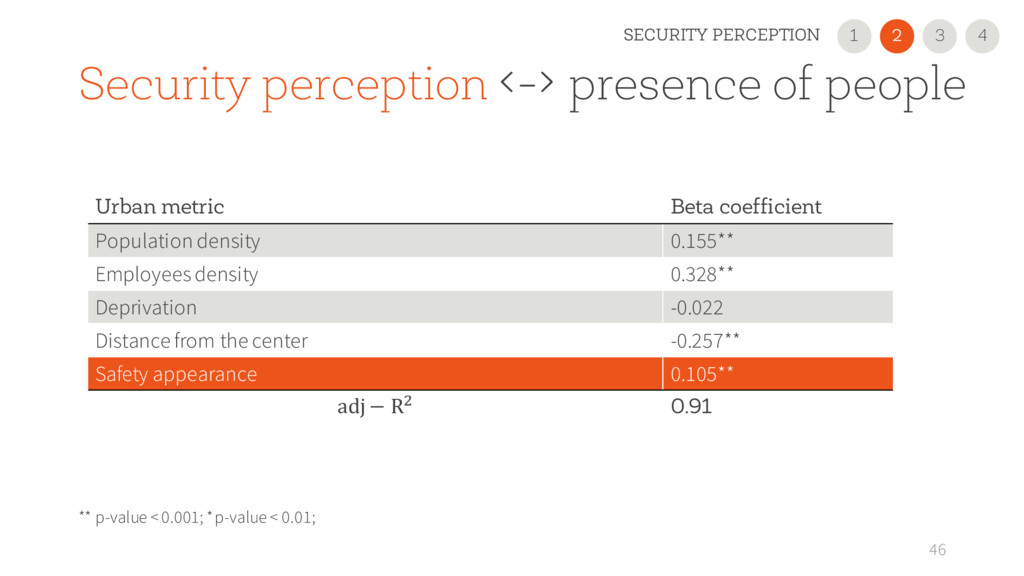
    coefficient Population density Employees density Deprivation Distance from the center Safety appearance adj − RN 0.91 ** p-value < 0.001; * p-value < 0.01; 1 SECURITY PERCEPTION 4 2 3
  41. 46 Urban metric Beta coefficient Population density 0.155** Employees density

    0.328** Deprivation -0.022 Distance from the center -0.257** Safety appearance 0.105** adj − RN 0.91 ** p-value < 0.001; * p-value < 0.01; Security perception <-> presence of people 1 SECURITY PERCEPTION 4 2 3
  42. 47 Urban metric Beta coefficient % of women (from census)

    0.001 Deprivation -0.005 Distance from the center -0.003 Safety appearance 0.020** adj − RN 0.65 ** p-value < 0.001; * p-value < 0.01; Security perception <-> women around 1 SECURITY PERCEPTION 4 2 3
  43. Visual elements for security perception 48 HIGH SAFETY PERCEPTION RANDOMLY

    OBSCURE PART OF THE IMAGE AND PREDICT 1 SECURITY PERCEPTION 4 2 3
  44. Visual elements for security perception 49 HIGH SAFETY PERCEPTION RANDOMLY

    OBSCURE PART OF THE IMAGE AND PREDICT 1 SECURITY PERCEPTION 4 2 3
  45. Result 50 De Nadai, Marco, et al. "Are Safer Looking

    Neighborhoods More Lively?: A Multimodal Investigation into Urban Life." ACM MM, 2016. Security perception can predict Presence of people 3 4 1 SECURITY PERCEPTION 2
  46. Crime OBJECTIVE CHARACTERISTICS Q: can we describe how physical characteristics

    influence crime? Q: can crime be predicted from the urban physical characteristics?
  47. Crime theory 52 CRIME Felson, M. (1994). Crime and everyday

    life: Insight and implications for society. Thousand Oaks, CA: Pine. 1 CRIME 4 2 3
  48. MOTIVATED OFFENDER Crime theory 53 CRIME Felson, M. (1994). Crime

    and everyday life: Insight and implications for society. Thousand Oaks, CA: Pine. 1 CRIME 4 2 3
  49. SUITABLE VICTIM MOTIVATED OFFENDER Crime theory 54 CRIME Felson, M.

    (1994). Crime and everyday life: Insight and implications for society. Thousand Oaks, CA: Pine. 1 CRIME 4 2 3
  50. ABSENCE OF CAPABLE GUARDIAN SUITABLE VICTIM MOTIVATED OFFENDER Crime theory

    55 CRIME Felson, M. (1994). Crime and everyday life: Insight and implications for society. Thousand Oaks, CA: Pine. 1 CRIME 4 2 3
  51. Crime: does place matters/predicts? 56 DATA • Web and Open

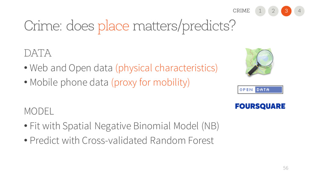
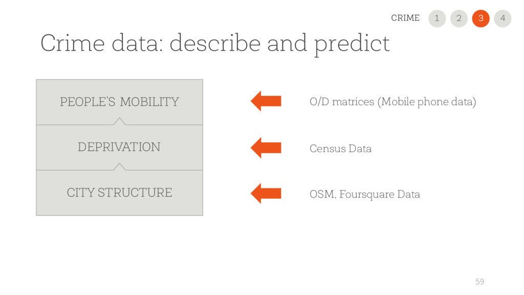
    data (physical characteristics) • Mobile phone data (proxy for mobility) MODEL • Fit with Spatial Negative Binomial Model (NB) • Predict with Cross-validated Random Forest 1 CRIME 4 2 3
  52. Crime data: describe and predict 59 PEOPLE’S MOBILITY CITY STRUCTURE

    DEPRIVATION O/D matrices (Mobile phone data) Census Data OSM, Foursquare Data 1 CRIME 4 2 3
  53. log ((% ) = ( ) + W + (

    Y Y P Y[K + ( + P\+ ] +[K The Negative Binomial Regression 60 1 CRIME 4 2 3
  54. log ((% ) = ( ) + W + (

    Y Y P Y[K + ( + P\+ ] +[K The Negative Binomial Regression 61 1 CRIME 4 2 3 Crime (Ground truth)
  55. log ((% ) = ( ) + W + (

    Y Y P Y[K + ( + P\+ ] +[K The Negative Binomial Regression 62 1 CRIME 4 2 3 Offset (population) Crime (Ground truth)
  56. log ((% ) = ( ) + W + (

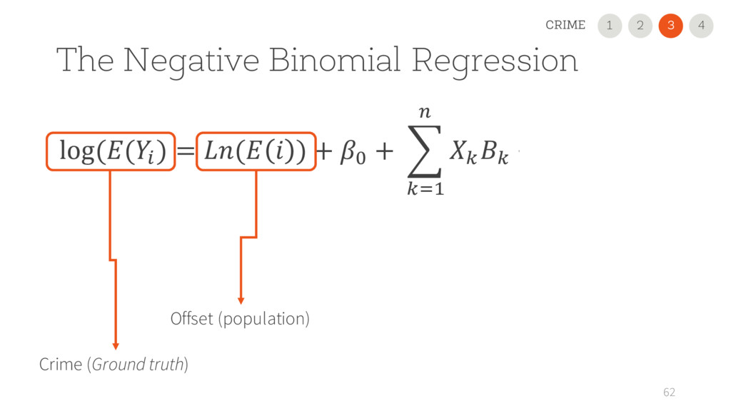
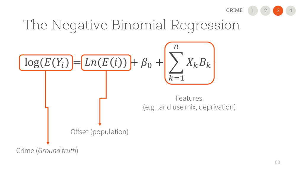
    Y Y P Y[K + ( + P\+ ] +[K The Negative Binomial Regression 63 1 CRIME 4 2 3 Offset (population) Crime (Ground truth) Features (e.g. land use mix, deprivation)
  57. log ((% ) = ( ) + W + (

    Y Y P Y[K + ( + P\+ ] +[K The Negative Binomial Regression 64 1 CRIME 4 2 3 “everything is related to everything else, but near things are more related than distant things.” Tobler's first law of geography
  58. log ((% ) = ( ) + W + (

    Y Y P Y[K + ( + P\+ ] +[K The Spatial Negative Binomial Regression 65 (significant) Spatial Eigenvectors 1 CRIME 4 2 3 Getis, Arthur, and Daniel A. Griffith. "Comparative spatial filtering in regression analysis." Geographical analysis 34.2 (2002): 130-140. • Eigenvector Spatial Filtering
  59. 66 Metric Social disorganization Daily routine City structure Full RMSE

    231.93 312.70 145.04 127.76 McFadderPseudo-R^2 0.077 0.085 0.113 0.143 Predict (nowcast) crime * 5-fold Cross-validation 1 CRIME 4 2 3 PRELIMINARY RESULTS
  60. Next? 68 4 • Add ambient population • Model Los

    Angeles, Boston, Providence • Describe commonality and differences 1 CRIME 2 3
  61. Structural layout ‘GENERATE’ THE CITY Q: can we formalize the

    desired qualities of a neighborhood and prototype it?
  62. Why simulate/generate a city • Endless discussions between stakeholders •

    Describe, predict => play • New insights 70 2 1 3 STRUCTURAL LAYOUT 4
  63. Why simulate/generate a city • Endless discussions between stakeholders •

    Describe, predict => play • New insights 71 2 1 3 STRUCTURAL LAYOUT 4
  64. Structural layout Design and enhance existing layouts • Learn from

    thousands of examples • Respecting the existing constraints • Build neighborhoods that work 72 2 1 3 STRUCTURAL LAYOUT 4
  65. Constructive Machine Learning Traditional approaches are limited • Model complex

    relations • Predict structured objects • Hard and soft constraints on the output 73 2 1 3 STRUCTURAL LAYOUT 4
  66. Constructive Machine Learning Traditional approaches are limited • Model complex

    relations • Predict structured objects • Hard and soft constraints on the output 74 2 1 3 STRUCTURAL LAYOUT 4 In collaboration with Andrea Passerini and MIT Media Lab
  67. Data mining to understand • Data mining as an inexpensive

    way to understand urban mechanisms • Predict social outcome from newly arise data • Deep understanding of city life through multi-modal data 76
  68. Limitations • Presence of data • Bias on data and

    models • Partial view • Domain adaptation (is it?) 77
  69. Multi-disciplinariety means discussions We collaborate with • Studio Carlo Ratti

    (MIT) • Humnetlab Marta Gonzalez (MIT) • Data-pop alliance, World Bank • Criminology researcher • MIT Media Lab Changing places 78
  70. We published CONFERENCES • De Nadai, M., et al. "The

    Death and Life of Great Italian Cities: A Mobile Phone Data Perspective." WWW, 2016. • De Nadai, M., et al. "Are Safer Looking Neighborhoods More Lively?: A Multimodal Investigation into Urban Life." ACM MM, 2016. JOURNALS • Barlacchi, G., De Nadai M., et al. A multi-source dataset of urban life in the city of Milan and the Province of Trentino. Scientific data, 2 (2015). • Centellegher, S., De Nadai M., et al. "The Mobile Territorial Lab: a multilayered and dynamic view on parents’ daily lives." EPJ Data Science 5.1 (2016). 80
  71. Safety perception: fix sparse votes • Learning safety perception, predict

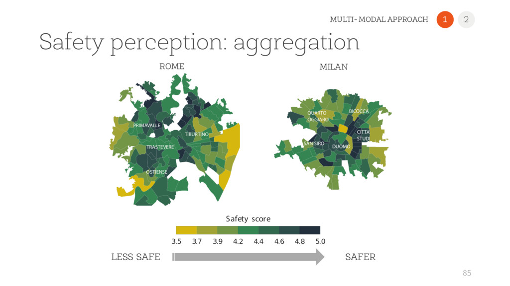
    in Rome and Milan • AlexNet CNN trained on Places205* 83 * B. Zhou, A. Lapedriza, J. Xiao, A. Torralba, and A. Oliva. “Learning Deep Features for Scene Recognition using Places Database.” NIPS, 2014. ** Ordonez, Vicente, and Tamara L. Berg. "Learning high-level judgments of urban perception.” ECCV, 2014. Model type State of art [**] Our model NY - NY 0.687 0.718 NY - Boston 0.701 0.734 Boston - Boston 0.718 0.744 Boston - NY 0.636 0.693 1 2 MULTI- MODAL APPROACH
  72. “What this [paper] does is put the facts on the

    table, and that’s a big step” … “It will bring up a lot of other research, in which, I don’t have any doubt, this will be put up as a seminal step” Luis Valenzuela, Urban Planner Harvard University Source: http://news.mit.edu/2016/quantifying-urban-revitalization-1024
  73. Safety perception: aggregation 85 1 2 MULTI- MODAL APPROACH 3.5

    3.7 3.9 4.2 4.4 4.6 4.8 5.0 Safety score DUOMO SAN SIRO QUARTO OGGIARO CITTA' STUDI BICOCCA TRASTEVERE TIBURTINO OSTIENSE PRIMAVALLE LESS SAFE SAFER ROME MILAN